An Intuitive Automated Modelling Interface
for Systems Biology

Abstract

We introduce a natural language interface for building stochastic $\pi$ calculus models of biological systems. In this language, complex constructs describing biochemical events are built from basic primitives of association, dissociation and transformation. This language thus allows us to model biochemical systems modularly by describing their dynamics in a narrative-style language, while making amendments, refinements and extensions on the models easy. We demonstrate the language on a model of Fc$\gamma$ receptor phosphorylation during phagocytosis. We provide a tool implementation of the translation into a stochastic $\pi$ calculus language, Microsoft Research’s SPiM.

1 Introduction

Modelling of biological systems by mathematical and computational techniques is becoming increasingly widespread in research on biological systems. In recent years, pioneered by Regev and Shapiro’s seminal work [16, 17], there has been a considerable amount of research on applying computer science technologies to modelling biological systems. Along these lines, various languages with stochastic simulation capabilities based on, for example, process algebra, term rewriting (see, e.g, [5, 7]) and Petri nets (see, e.g., [19, 9]) have been proposed. However, expressing biological knowledge in specialised modelling languages often requires a simultaneous understanding of the biological system and expert knowledge of the modelling language. Isolating and communicating the biological knowledge to build models for simulation and analysis is a challenging task both for wet-lab biologists and modellers.

Writing programs in simulation languages requires specialised training, and it is difficult even for the experts when complex interactions between biochemical species in biological systems are considered: the representation of different states of a biochemical species with respect to all its interaction capabilities results in an exponential blow up in the number of states. For example, when a protein with $n$ different interaction sites is being modelled, this results in $2^{n}$ states, which needs to be represented in the model. Enumerating all these states by hand, also without inserting typos is a difficult task.

To this end, we introduce an intuitive front-end interface language for building process algebra models of biological systems: process algebras are languages that have originally been designed to formally describe complex reactive computer systems. Due to the resemblance between these computer systems and biological systems, process algebra have been recently used to model biological systems. An important feature of the process algebra languages is the possibility to describe the components of a system separately and observe the emergent behaviour from the interactions of the components (see, e.g., [1, 2]).

Our focus here is on $\pi$ calculus [12], which is a broadly studied process algebra, also because of its compactness, generality, and flexibility. Because biological systems are typically highly complex and massively parallel, the $\pi$ calculus is well suited to describe their dynamics. In particular, it allows the components of a biological system to be modelled independently, rather than modelling individual reactions. This allows large models to be constructed by composition of simple components. $\pi$ calculus also enjoys an expressive power in the setting of biological models that exceeds, e.g., Petri nets [3].

In the following, we present a language that consists of basic primitives of association, dissociation and transformation. We impose certain consistency constraints on these primitive expressions, which are required for the models that describe the dynamics of biochemical processes. We give a translation algorithm into stochastic $\pi$ calculus. Based on this, we present the implementation of a tool for automated translation of models into Microsoft Research’s stochastic simulation language $\mathsf{SPiM}$ [14, 13], which can be used to run stochastic simulations on $\pi$ calculus models. We demonstrate the language on a model of Fc$\gamma$ receptor phosphorylation during phagocytosis. The implementation of the translation tool as well as further information is available for download at our website .

2 Species, Sites, Sentences and Models

We follow the abstraction of biochemical species as stateful entities with connectivity interfaces to other species: a species can have a number of sites through which it interacts with other species, and changes its state as a result of the interactions [6, 11]. In Section 4, we use this idea to design a natural language-like syntax for building models. The models written in this language are then automatically translated into a $\mathsf{SPiM}$ program by a translation algorithm. This is done by mapping the sentences of the language into events constructed from the basic primitives, which are then compiled into executable process expressions in the $\mathsf{SPiM}$ language.

There is a countable set of species $A,B,C,\ldots$. Each species has a number of sites $a,b,c,\ldots$ with which it can bind to other species or unbind from other species when they are already bound. We write sentences that describe the ‘behaviour’ of each species with respect to their sites. There are three kinds of sentences, i.e., associations, dissociations, and transformations. We define the sentences as

$$\langle\,\mathsf{type},(A,a),\,(B,b),\,\textit{Pos},\,\textit{Neg},\,r\,\rangle$$

where $\mathsf{type}\in\{$association, dissociation, transformation$\}$ is the type of the sentence. The pairs $(A,a)$ and $(B,b)$ are called the body of the sentence. The sets Pos and Neg are called the conditions of the sentences. $(A,a)$ and $(B,b)$ are pairs of species and sites, and Pos and Neg are sets of such pairs of species and sites. If the sentence is an association, it describes the event where the site $a$ on species $A$ associates to the site $b$ on species $B$ if the sites on species in Pos are already bound and those in Neg are already unbound. If it is a dissociation sentence, it describes the dissociation of the site $a$ on species $A$ from the site $b$ on species $B$. A transformation sentence describes the event of species $A$ transforming into species $B$, where $B$ can be empty. In this case, this describes the decay of species $A$. In transformation sentences, sites $a$ and $b$ must be empty, since transformations are site independent. $r\in\mathbb{R}^{+}$ denotes the rate of the event that the sentence describes. Then a model $\mathcal{M}$ is a set of such sentences. In Section 4, we give a representation of these sentences in natural-language. For example, a sentence of the form $\langle\,\textit{association},(A,a),\,(B,b),\,\{(A,c)\},\,\{\,\},\,1.0\,\rangle$ is given with the following English sentence.

site a on A associates site b on B with rate 1.0 if site c on A is bound

We denote with $\mathsf{species}(\mathcal{M})$ all the species occurring in the body of the sentences of $\mathcal{M}$. The function $\mathsf{sites}(\mathcal{M},A)$ denotes the sites of the species $A$ that occur in the body of all the sentences of $\mathcal{M}$. $\mathsf{sites}(\textit{Pos},A)$ denotes the sites of the species $A$ in Pos (similarly for Neg). For any set $\mathcal{A}$, $\wp(\mathcal{A})$ denotes the powerset of $\mathcal{A}$.

2.1 Conditions on Sentences

Given a model $\mathcal{M}$, we impose several conditions on its sentences.

1. Sentences contain relevant species. The species in the condition of each sentence must be a subset of those in the body of the sentence.

2. Conditions of the sentences are consistent. For every sentence of the form
   $\langle\,\mathsf{type},(A,a),\,(B,b),\,\textit{Pos},\,\textit{Neg},\,r\,\rangle$, we have that $\textit{Pos}\cap\textit{Neg}=\emptyset$.

3. All the sites in the conditions are declared in the model. For every sentence of the form $\langle\,\mathsf{type},(A,a),\,(B,b),\,\textit{Pos},\,\textit{Neg},\,r\,\rangle$, we have that $\mathsf{sites}(\textit{Pos},A)\subseteq\mathsf{sites}(\mathcal{M},A)$,
   $\mathsf{sites}(\textit{Neg},A)\subseteq\mathsf{sites}(\mathcal{M},A)$, $\mathsf{sites}(\textit{Pos},B)\subseteq\mathsf{sites}(\mathcal{M},B)$ and $\mathsf{sites}(\textit{Neg},B)\subseteq\mathsf{sites}(\mathcal{M},B)$.

4. Association sentences associate unbound species. For every association sentence
   $\langle\,\textit{association},(A,a),\,(B,b),\,\textit{Pos},\,\textit{Neg},\,r\,\rangle$, we have that $(A,a)$, $(B,b)\in\textit{Neg}$.

5. Dissociation sentences dissociate bound species. For every dissociation sentence
   $\langle\,\textit{dissociation},(A,a),\,(B,b),\,\textit{Pos},\,\textit{Neg},\,r\,\rangle$, we have that $(A,a)$, $(B,b)\in\textit{Pos}$.

6. Transformation sentences are unbound at all sites. For every transformation sentence
   $\langle\,\textit{transformation},A,\,B,\,\textit{Pos},\,\textit{Neg},\,r\,\rangle$, we have that $\textit{Pos}=\emptyset$ and $\textit{Neg}=\{(A,x)\,|\,x\in\mathsf{sites}(\mathcal{M},A)\}$.

When these conditions hold, we can map the sentences of a model to another representation where the role of the conditions become more explicit. In the following, for a model $\mathcal{M}$, we describe the states of its species as subsets of its sites, where bound sites are included in the set describing the state. For example, for a species $A$ with binding sites $\mathsf{sites}(\mathcal{M},A)=\{a,b\}$, the set $\wp(\mathsf{sites}(\mathcal{M},A))=\{\{\},\{a\},\{b\},\{a,b\}\}$ is the set of all its states. Then $\{a\}$ is the state where site $a$ on $A$ is bound and site $b$ on $A$ is unbound. We map each sentence $\langle\,\mathsf{type},(A,a),\,(B,b),\,\textit{Pos},\,\textit{Neg},\,r\,\rangle$ to a sentence of the form

$$\langle\,\mathsf{type},(A,a),\,(B,b),\,\mathsf{states}(A),\,\mathsf{states}(B),\,r\,\rangle$$

where $\mathsf{states}(A)$ and $\mathsf{states}(B)$ are obtained as follows.

$$\mathsf{states}(A)=\{\,\mathcal{S}\in\wp(\mathsf{sites}(\mathcal{M},A))\;|\;(\,(A,x)\in\textit{Pos}\Rightarrow x\in\mathcal{S}\,)\land(\,x\in\mathcal{S}\Rightarrow(A,x)\notin\textit{Neg}\,)\,\}$$

This representation allows us to impose another condition on the sentences:

1. There are no overlapping conditions in the sentences. For any two sentences of a model $\mathcal{M}$ of the form $\langle\,\mathsf{type}_{1},(A,a),\,(B,b),\,\textit{Pos}_{1},\,\textit{Neg}_{1},\,r\,\rangle$ and $\langle\,\mathsf{type}_{2},(A,a),\,(B,b),\,\textit{Pos}_{2},\,\textit{Neg}_{2},\,r\,\rangle$ where $\mathsf{type}_{1}=\mathsf{type}_{2}$, we obtain $\mathsf{states}(A)_{1}$ and $\mathsf{states}(B)_{1},$ for the first and $\mathsf{states}(A)_{2}$ and $\mathsf{states}(B)_{2},$ for the second sentence. Then we have that

   – if $\mathsf{states}(A)_{1}=\mathsf{states}(A)_{2}$ then it must be that $\mathsf{states}(B)_{1}\,\cap\;\mathsf{states}(B)_{2}=\emptyset$;

   – if $\mathsf{states}(B)_{1}=\mathsf{states}(B)_{2}$ then it must be that $\mathsf{states}(A)_{1}\,\cap\;\mathsf{states}(A)_{2}=\emptyset$;

   – if $\mathsf{states}(A)_{1}\neq\mathsf{states}(A)_{2}$ and $\mathsf{states}(B)_{1}\neq\mathsf{states}(B)_{2}$ then it must be that
   $\mathsf{states}(A)_{1}\,\cap\;\mathsf{states}(A)_{2}=\emptyset$ and $\mathsf{states}(B)_{1}\,\cap\;\mathsf{states}(B)_{2}=\emptyset$.

Example 1

Consider the models $\mathcal{M}_{1}$.

$$\begin{array}[]{l}\mathcal{M}_{1}=\{\,\langle\,\textit{association},(A,a),\,(B,b),\,\{(B,f)\},\,\{(C,c),\,(A,a),(B,f)\},\,1.0\,\rangle,\\ \quad\quad\quad\;\>\>\langle\,\textit{dissociation},(A,a),\,(B,b),\,\{(B,b)\},\,\{\},\,1.0\,\rangle,\\ \quad\quad\quad\;\>\>\langle\,\textit{transformation},A,\,B,\,\{\},\,\{\},\,1.0\,\rangle,\\ \quad\quad\quad\;\>\>\langle\,\textit{association},(D,d),\,(E,e),\,\{\},\,\{(D,d),\,(E,e)\},\,2.0\,\rangle,\\ \quad\quad\quad\;\>\>\langle\,\textit{association},(D,d),\,(E,e),\,\{\},\,\{(D,d),\,(E,e)\},\,4.0\,\rangle\,\}\end{array}$$

This model does not fulfill any of the conditions above: in the first sentence, (1.) $C\notin\{A,B\}$; (2.) $(B,f)\in\textit{Pos}$ and $(B,f)\in\textit{Neg}$; (3.) $f\notin\{b\}$; (4.) $(B,b)\notin\{(C,c),\,(A,a),(B,f)\}$. In the second sentence, (5.) $(A,a)\notin\{(B,b)\}$. In the third sentence, (6.) $\{\}\neq\{(A,a)\}$. (7.) In the fourth and fifth sentences, $\mathsf{states}(D)_{1}=\{\{\}\}=\mathsf{states}(D)_{2}$ and $\mathsf{states}(E)_{1}=\{\{\}\}=\mathsf{states}(E)_{2}$.

Example 2

The model $\mathcal{M}_{2}$ fulfills all the conditions above.

$$\begin{array}[]{l}\mathcal{M}_{2}=\{\,\langle\,\textit{association},(A,a_{1}),\,(B,b),\,\{\},\,\{(A,a_{1}),(B,b)\},\,1.0\,\rangle,\\ \quad\quad\quad\;\>\>\langle\,\textit{association},(A,a_{2}),\,(C,c),\,\{\},\,\{(A,a_{2}),(C,c)\},\,1.0\,\rangle,\\ \quad\quad\quad\;\>\>\langle\,\textit{dissociation},(A,a_{1}),\,(B,b),\,\{(A,a_{1}),\,(A,a_{2}),\,(B,b)\},\,\{\}\},\,2.0\,\rangle,\\ \quad\quad\quad\;\>\>\langle\,\textit{dissociation},(A,a_{1}),\,(B,b),\,\{(A,a_{1}),\,(B,b)\},\,\{(A,a_{2})\}\},\,4.0\,\rangle\,\}\end{array}$$

3 Translation into Stochastic $\pi$ calculus

We use the representation of the states of species as sets of their sites to map models to stochastic $\pi$ calculus specifications. For this purpose, we first map each model to a compile map. Let us first recall some of the definitions of stochastic $\pi$ calculus, implemented in SPiM, as they can be found in [13].

3.1 Stochastic $\pi$ calculus

Definition 3

Syntax of stochastic $\pi$ calculus. Below fn$(P)$ denotes the set of names that are free in $P$.

$$\begin{array}[]{ll}\begin{array}[]{rll}E::=&\quad\emptyset&\quad\textrm{Empty}\\[2.0pt] |&\quad E,X(\tilde{m})=P&\quad\textrm{Definition}\\[2.0pt] |&&\quad\textrm{fn}(P)\subseteq\tilde{m}\\[2.0pt] \\ \end{array}&\quad\begin{array}[]{rll}P,Q::=&\quad\Sigma&\quad\textrm{Summation}\\[2.0pt] |&\quad X(\tilde{n})&\quad\textrm{Instance}\\[2.0pt] |&\quad P\,|\,Q&\quad\textrm{Parallel}\\[2.0pt] |&\quad\verb+new+\,x\;P&\quad\textrm{Restriction}\end{array}\\ \\ \begin{array}[]{rll}\Sigma::=&\quad\mathbf{0}&\quad\textrm{Null}\\[2.0pt] |&\quad\pi\verb+;+P+\Sigma&\quad\textrm{Action}\\[2.0pt] \\ \end{array}&\quad\begin{array}[]{rll}\pi::=&\quad?x(\tilde{m})&\quad\textrm{Input}\\[2.0pt] |&\quad!x(\tilde{n})&\quad\textrm{Output}\\[2.0pt] |&\quad\tau_{r}&\quad\textrm{Delay}\end{array}\end{array}$$

Expressions above are considered equivalent up to the least congruence relation given by the equivalence relation $\equiv$ defined as follows.

$$\begin{array}[]{ll}\begin{array}[]{rll}P\;|\;\mathbf{0}&\equiv&P\\[2.0pt] P\;|\;Q&\equiv&Q\;|\;P\\[2.0pt] P\;|\;(Q\;|\;R)&\equiv&(P\;|\;Q)\;|\;R\\[2.0pt] X(\tilde{n})&\equiv&P_{\{\tilde{n}/\tilde{m}\}}\textrm{ if }X(\tilde{m})=P\end{array}&\quad\begin{array}[]{rll}\verb+new+\,x\;\mathbf{0}&\equiv&\mathbf{0}\\[2.0pt] \verb+new+\,x\;\verb+new+\,y\;P&\equiv&\verb+new+\,y\;\verb+new+\,x\;P\\[2.0pt] \verb+new+\,x\;(P\;|\;Q)&\equiv&P\;|\;\verb+new+\,x\;Q\textrm{ if }x\notin\textrm{fn}(P)\\ \\ \end{array}\end{array}$$

3.2 Compile Maps

We map models into compile maps, denoted with $\mathcal{C}$. A compile map is a set of expressions that we call process descriptions for each species $A\in\mathsf{species}(\mathcal{M})$. For a model $\mathcal{M}$, the process description of species $A\in\mathsf{species}(\mathcal{M})$, denoted with $\mathsf{P}(A)$, is the pair $\langle A,\,\mathsf{actions}(A)\rangle$. Here, $\mathsf{actions}(A)$ is the set collecting $\mathsf{actions}(A,\mathcal{S})$ for every $\mathcal{S}\in\wp(\mathsf{sites}(\mathcal{M},A))$.

$$\mathsf{actions}(A,\mathcal{S})=\langle\mathcal{S},\mathsf{assoc}(A,\mathcal{S}),\mathsf{dissoc}(A,\mathcal{S}),\mathsf{transform}(A,\mathcal{S})\rangle$$

We define $\mathsf{assoc}(A,\mathcal{S})$ as the set of $\mathsf{assoc}(A,\mathcal{S},a)$ for every $a\in\mathsf{sites}(\mathcal{M},A)$.

$$\mathsf{assoc}(A,\mathcal{S},a)=\langle a,\mathsf{assocPartners}{(A,\mathcal{S},a)}\rangle$$

where $\mathsf{assocPartners}(A,\mathcal{S},a)$ is the set

$$\begin{array}[]{l}\{\langle B,b,\mathsf{states}(B),r\rangle\;|\\[2.0pt] \qquad\qquad\quad(\,\langle\,\textit{association},\,(A,a),\,(B,b),\,\textit{Pos},\,\textit{Neg},\,r\,\rangle\in\mathcal{M}\;\land\;\mathcal{S}\in\mathsf{states}(A)\,)\\[2.0pt] \qquad\quad\quad\lor\;(\,\langle\,\textit{association},\,(B,b),\,(A,a),\,\textit{Pos},\,\textit{Neg},\,r\,\rangle\in\mathcal{M}\;\land\;\mathcal{S}\in\mathsf{states}(A)\,)\,\}\,.\end{array}$$

We define $\mathsf{dissoc}(A,\mathcal{S})$, similarly, as the set of $\mathsf{dissoc}(A,\mathcal{S},a)$ for every $a\in\mathsf{sites}(\mathcal{M},A)$.

$$\mathsf{dissoc}(A,\mathcal{S},a)=\langle a,\mathsf{dissocPartners}{(A,\mathcal{S},a)}\rangle$$

where $\mathsf{dissocPartners}(A,\mathcal{S},a)$ is the set

$$\begin{array}[]{l}\{\langle B,b,\mathsf{states}(B),r\rangle\;|\\[2.0pt] \qquad\qquad\quad(\,\langle\,\textit{dissociation},\,(A,a),\,(B,b),\,\textit{Pos},\,\textit{Neg},\,r\,\rangle\in\mathcal{M}\;\land\;\mathcal{S}\in\mathsf{states}(A)\,)\\[2.0pt] \qquad\quad\quad\lor\;(\,\langle\,\textit{dissociation},\,(B,b),\,(A,a),\,\textit{Pos},\,\textit{Neg},\,r\,\rangle\in\mathcal{M}\;\land\;\mathcal{S}\in\mathsf{states}(A)\,)\,\}\,.\end{array}$$

If $\mathcal{S}=\emptyset$, the set $\mathsf{transform}(A,\mathcal{S})$ is defined as

$$\{\langle B,r\rangle\;|\;(\,\langle\,\textit{transformation},\,A,\,B,\,\textit{Pos},\,\textit{Neg},\,r\,\rangle\in\mathcal{M}\,\}\,.$$

Otherwise, it is $\emptyset$.

Example 4

Consider the model $\mathcal{M}_{2}$ in Example 2. We have that the compile map $\mathcal{C}_{2}$ for this model is as follows.

$$\begin{array}[]{ll}\{\;\langle\,A,\,\{&\!\!\!\!\!\langle\,\{\},\,\{(a_{1},\{(B,b,\{\{\}\},1.0)\}),\,(a_{2},\{(C,c,\{\{\}\},1.0)\},\,\{\},\,\{\}\,\rangle\,,\\[2.0pt] &\!\!\!\!\!\langle\,\{a_{1}\},\,\{(a_{2},\{(C,c,\{\{\}\},1.0)\},\,\{(B,b,\{\{b\}\},4.0)\},\,\{\}\,\rangle\,,\\[2.0pt] &\!\!\!\!\!\langle\,\{a_{2}\},\,\{(a_{1},\{(B,b,\{\{\}\},1.0)\},\,\{\},\,\{\}\,\rangle\,,\\[2.0pt] &\!\!\!\!\!\langle\,\{a_{1},\,a_{2}\},\,\{\},\,\{(B,b,\{\{b\}\},2.0)\},\,\{\}\,\rangle\;\}\,\rangle\,,\\[3.0pt] \;\;\;\langle\,B,\,\{&\!\!\!\!\!\langle\,\{\},\,\{(b,\{(A,a_{1},\{\{\},\,\{a_{2}\}\},1.0)\},\,\{\},\,\{\}\,\rangle\,,\\[2.0pt] &\!\!\!\!\!\langle\,\{b\},\,\{\},\,\{(b,\{(A,a_{1},\{\{a_{1}\}\},4.0),\,(A,a_{1},\{\{a_{1},\,a_{2}\}\},2.0)\},\,\{\}\,\rangle\;\}\,\rangle\,,\\[3.0pt] \;\;\;\langle\,C,\,\{&\!\!\!\!\!\langle\,\{\},\,\{(a_{1},\{(A,a_{2},\{\{\},\,\{a_{1}\}\},1.0)\ \},\,\{\},\,\{\}\,\rangle\,,\\[2.0pt] &\!\!\!\!\!\langle\,\{c\},\,\{\},\,\{\},\,\{\}\,\rangle\;\}\,\rangle\,\}\end{array}$$

3.3 From Compile Maps to Stochastic $\pi$ calculus

We construct a $\pi$ calculus specification from the compile map $\mathcal{C}$ of a model $\mathcal{M}$. For each species $A\in\mathsf{species}(\mathcal{M})$, we map the process description $\mathsf{P}(A)$ to a process specification in stochastic $\pi$ calculus. Let

$$\mathsf{P}(A)=\langle A,\{\,\mathsf{actions}(A,\mathcal{S}_{1}),\ldots,\mathsf{actions}(A,\mathcal{S}_{n})\,\}\rangle$$

where $\wp(\mathsf{sites}(\mathcal{M},A))=\{\mathcal{S}_{1},\ldots,\mathcal{S}_{n}\}$, that is, the powerset of set of sites of $A$. Thus, there are $n$ process specifications for the species $A$, some of which may be empty. Each process specification for each state $\mathcal{S}$ of $A$ is of the following syntactic form.

$$\begin{array}[]{lll}\textit{process declaration}&\>\textrm{``= (''}&\textit{ local channel declarations}\\[2.0pt] &&\textit{ association specifications}\\[2.0pt] &\;\;\;\textrm{``+''}&\textit{ dissociation specifications}\\[2.0pt] &\;\;\;\textrm{``+''}&\textit{ transformation specifications}\;\;\textrm{``)''}\end{array}$$

The idea here is that each set of sites of a species $A$ denotes the state where the sites in the set are bound. Thus the powerset of the set of sites of a species denotes the set of all its states. Now, let us obtain the process expression for each state $\mathcal{S}_{i}$ with respect to $\mathsf{actions}(A,\mathcal{S}_{i})$ where $1\leq i\leq n$. Let us consider $\mathcal{S}_{i}=\{a_{1},\ldots,a_{k}\}$ of $A$ with

$$\mathsf{actions}(A,\mathcal{S}_{i})=\langle\mathcal{S}_{i}\,,\mathsf{assoc}(A,\mathcal{S}_{i}),\mathsf{dissoc}(A,\mathcal{S}_{i}),\mathsf{transform}(A,\mathcal{S}_{i})\rangle\,.$$

Process declaration

The expression for process declaration is a process name with its list of parameters. It is delivered by the dissociation sentences in $\mathcal{M}$ and $\mathcal{S}_{i}=\{a_{1},\ldots,a_{k}\}$. For every $a_{j}\in\mathcal{S}_{i}$, consider the set

$$\begin{array}[]{l}\!\!\!\!\!\mathcal{R}(A,a_{j})=\\[2.0pt] \!\!\!\!\!\{(a_{j},\,(r/2))\;|\,\langle\textit{dissociation},(A,a_{j}),(B,b),\,\textit{Pos},\,\textit{Neg},\,r\rangle\in\,\mathcal{M}\,\}\;\cup\\[2.0pt] \!\!\!\!\!\,\quad\{(a_{j},\,(r/2))\;|\,\langle\textit{dissociation},(B,b),(A,a_{j}),\,\textit{Pos},\,\textit{Neg},\,r\rangle\,\in\,\mathcal{M}\,\}\;\cup\\[2.0pt] \!\!\!\!\!\qquad\,\,\quad\{(a_{j},\,1.0)\;|\,\langle\textit{dissociation},(B,b),(A,a_{j}),\,\textit{Pos},\,\textit{Neg},\,r\rangle\,\notin\,\mathcal{M}\;\land\\[2.0pt] \qquad\qquad\quad\qquad\;\;\quad\langle\textit{dissociation},(A,a_{j}),(B,b),\,\textit{Pos},\,\textit{Neg},\,r\rangle\,\notin\,\mathcal{M}\}\,.\end{array}$$

We associate each element of the set $\mathcal{R}(A,a_{j})$ a unique label $s\in\mathbb{N}^{+}$ and obtain $\mathcal{R}^{\prime}(A,a_{j})$. Then if $\mathcal{R}^{\prime}(A,a_{j})=\{(a_{j},\,r_{1},\,1),\ldots,(a_{j},\,r_{\ell},\,\ell)\,\}$ we write the process declaration for $A$ at state $\mathcal{S}_{i}=\{a_{1},\ldots,a_{k}\}$ as follows.

$$A_{i}({a_{1}}{1},\ldots,{a_{1}}{\ell_{1}},\ldots\ldots,{a_{k}}{1},\ldots,{a_{k}}{\ell_{k}})$$

Example 5

For the state $\mathcal{S}_{2}=\{a_{1}\}$ of species $A$ of Example 2, we have the process declaration below, since we have that $\,\mathcal{R}^{\prime}(A,a_{1})=\{(a_{1},2.0,1),(a_{1},1.0,2)\}$.

$$A_{2}({a_{1}}{1},{a_{1}}{2})$$

Local channel declarations

These expressions are delivered by the dissociation sentences in $\mathcal{M}$ and the $\mathsf{assoc}(A,\mathcal{S}_{i})$. That is, for every

$$\mathsf{assoc}(A,\mathcal{S}_{i},a_{j})=\langle\,a_{j},\,\mathsf{assocPartners}(A,\mathcal{S}_{i},a_{j})\,\rangle\in\mathsf{assoc}(A,\mathcal{S}_{i})\,,$$

and for every $\langle\,B,b,\mathsf{states}(B),\,r\,\rangle\in\mathsf{assocPartners}(A,\mathcal{S}_{i},a_{j})$ consider the set

$$\begin{array}[]{l}\!\!\!\!\!\mathcal{U}(A,a_{j},B,b)=\\[2.0pt] \!\!\!\!\!\{(a_{j},\,(r/2))\;|\,\langle\textit{dissociation},(A,a_{j}),(B,b),\,\textit{Pos},\,\textit{Neg},\,r\rangle\in\,\mathcal{M}\,\land\,a_{j}\prec b\,\}\;\cup\\[2.0pt] \!\!\!\!\!\,\quad\{(a_{j},\,(r/2))\;|\,\langle\textit{dissociation},(B,b),(A,a_{j}),\,\textit{Pos},\,\textit{Neg},\,r\rangle\,\in\,\mathcal{M}\,\land\,a_{j}\prec b\,\}\;\cup\\[2.0pt] \!\!\!\!\!\,\,\quad\quad\{(a_{j},\,1.0)\;|\,\langle\textit{dissociation},(B,b),(A,a_{j}),\,\textit{Pos},\,\textit{Neg},\,r\rangle\,\notin\,\mathcal{M}\;\land\\[2.0pt] \quad\quad\qquad\qquad\;\;\quad\langle\textit{dissociation},(A,a_{j}),(B,b),\,\textit{Pos},\,\textit{Neg},\,r\rangle\,\notin\,\mathcal{M}\,\land\,a_{j}\prec b\,\}\end{array}$$

where $\prec$ denotes a lexicographic order on sites. We associate each element of the set $\mathcal{U}(A,a_{j},B,b)$ a unique label $s\in\mathbb{N}^{+}$ to obtain $\mathcal{U}^{\prime}(A,a_{j},B,b)$. Then if

$$\mathcal{U}^{\prime}(A,a_{j},B,b)=\{(a_{j},\,r_{1},\,1),\ldots,(a_{j},\,r_{\ell},\,\ell)\}$$

then we write the channel declarations for $\mathsf{assoc}(A,\mathcal{S}_{i},a_{j})$ as follows.

$$\verb+new +{a_{j}}{1}\verb+@+r_{1}\quad\ldots\quad\verb+new +{a_{j}}{\ell}\verb+@+r_{\ell}$$

Example 6

For the state $\mathcal{S}_{2}=\{a_{1}\}$ of species $A$ of Example 2, we have the channel declarations below, since we have that $\mathcal{U}^{\prime}(A,a_{2},B,b)=\{(a_{2},1.0,1)\}$.

$$\verb+new +{a_{2}}{1}\verb+@+1.0$$

Association specifications

The expression for association specifications for species $A$ at state $\mathsf{assoc}(A,\mathcal{S}_{i})$ is delivered by $\mathsf{assoc}(A,\mathcal{S}_{i})$. For every

$$\langle\,a_{j},\,\mathsf{assocPartners}(A,\mathcal{S}_{i},a_{j})\,\rangle\in\mathsf{assoc}(A,\mathcal{S}_{i}),$$

and for every $\langle\,B,b,\mathsf{states}(B),\,r\,\rangle\in\mathsf{assocPartners}(A,\mathcal{S}_{i},a_{j})$ consider the set

$$\begin{array}[]{l}\!\!\!\!\!\mathcal{B}(A,a_{j},B,b)=\\[2.0pt] \quad\quad\!\!\!\!\!\{(\verb+!+a_{j}b,\,r)\;|\,\langle(B,b),\,\mathsf{states}(B),\,r\rangle\in\mathsf{assocPartners}(A,\mathcal{S}_{i},a_{j})\,\land\,a_{j}\prec b\,\}\;\,\cup\\[2.0pt] \quad\quad\quad\!\!\!\!\!\{(\verb+?+ba_{j},\,r)\;|\,\langle(B,b),\,\mathsf{states}(B),\,r\rangle\in\mathsf{assocPartners}(A,\mathcal{S}_{i},a_{j})\,\land\,b\prec a_{j}\,\}\,.\end{array}$$

We associate each element of the set $\mathcal{B}(A,a_{j},B,b)$ a unique label $s\in\mathbb{N}^{+}$ and obtain $\mathcal{B}^{\prime}(A,a_{j},B,b)$. Association of site $a_{j}$ on $A$ results in the state $\mathcal{S}_{i^{\prime}}=\mathcal{S}_{i}\cup\{a_{j}\}$. For each element of $(\verb+!+a_{j}b,r_{s},s)\in\mathcal{B}^{\prime}(A,a_{j},B,b)$ we write the following, composed by +.

$$\verb+!+a_{j}bs(a_{j}1,\ldots,a_{j}\ell)\verb+;+\textit{continuation}\;$$

The association channel names, such as $a_{j}bs$ here, are also declared as global channel declarations, preceding all the process declarations. The continuation is written for A in $\mathcal{S}_{i^{\prime}}$ as for process declarations above, however we write nil for the channel names for those associations of site $a_{j}$ on $A$ with some site $b^{\prime}\neq b$. Here, nil is the nil-dissociation channel with rate $0$. We obtain $a_{j}1,\ldots,a_{j}\ell$ from the set $\mathcal{U}(A,a_{j},B,b)$ as in channel declarations.

Example 7

For the state $\mathcal{S}_{2}=\{a_{1}\}$ of species $A$ of Example 2, we have the following association specifications.

$$!a2c1(a_{2})\verb+;+A3(a_{1}1,a_{1}2,a_{2})$$

Dissociation specifications

The expression for dissociation specifications for species $A$ at state $\mathsf{assoc}(A,\mathcal{S}_{i})$ is delivered by $\mathsf{dissoc}(A,\mathcal{S}_{i})$. For every

$$\langle\,a_{j},\,\mathsf{dissocPartners}(A,\mathcal{S}_{i},a_{j})\,\rangle\in\mathsf{dissoc}(A,\mathcal{S}_{i}),$$

and for every $\langle\,B,b,\mathsf{states}(B),\,r\,\rangle\in\mathsf{dissocPartners}(A,\mathcal{S}_{i},a_{j})$ consider the set

$$\begin{array}[]{l}\!\!\!\!\!\mathcal{G}(A,a_{j},B,b)=\\[2.0pt] \quad\quad\!\!\!\!\!\{(\verb+!+a_{j},\,r)\;|\,\langle(B,b),\,\mathsf{states}(B),\,r\rangle\in\mathsf{dissocPartners}(A,\mathcal{S}_{i},a_{j})\,\land\,a_{j}\prec b\,\}\;\,\cup\\[2.0pt] \quad\quad\quad\!\!\!\!\!\{(\verb+?+b,\,r)\;|\,\langle(B,b),\,\mathsf{states}(B),\,r\rangle\in\mathsf{dissocPartners}(A,\mathcal{S}_{i},a_{j})\,\land\,b\prec a_{j}\,\}\,.\end{array}$$

We associate each element of the set $\mathcal{G}(A,a_{j},B,b)$ a unique label $s\in\mathbb{N}^{+}$ and obtain $\mathcal{G}^{\prime}(A,a_{j},B,b)$. Dissociation of $a_{j}$ on $A$ results in the state $\mathcal{S}_{i^{\prime}}=\mathcal{S}_{i}\setminus\{a_{j}\}$. For each $(\verb+!+a_{j},r_{s},s)\in\mathcal{G}^{\prime}(A,a_{j},B,b)$ we write the following, composed by “+”.

$$\verb+!+a_{j}s\verb+;+\textit{continuation}\;\verb- + -\>\verb+?+a_{j}s\verb+;+\textit{continuation}$$

The continuation is written for A in $\mathcal{S}_{i^{\prime}}$ as for process declarations above.

Example 8

For the state $\mathcal{S}_{2}=\{a_{1}\}$ of species $A$ of Example 2, we have the following dissociation specifications.

$$\verb+!+a_{1}1\verb+;+A_{1}()\verb- + -\verb+?+a_{1}1;A_{1}()$$

Transformation specifications

The expression for transformation specifications for species $A$ is given only if the state $\mathcal{S}=\{\}$. In that case, for $\mathsf{transfrom}(A,\{\})=\{(B_{1},r_{1}),\ldots,(B_{k},r_{k})\}$ we write

$$\verb+delay@+r_{1}\verb+;+B_{1}()\verb- + -\ldots\verb- + -\verb+delay@+r_{k}\verb+;+B_{k}()$$

4 Syntax of the Language

The syntax of the language is defined in BNF notation, where optional elements are enclosed in braces as {Optional}. A model (description) consists of sentences of the following form.

Model	$::=$	Sentence1 … Sentence${}_{m}\qquad m\geq 1$
Sentence	$::=$	Association
	$|$	Dissociation
	$|$	Transformation
	$|$	Decay
	$|$	Phosphorylation
	$|$	Dephosphorylation
Association	$::=$	Site on Species associates Site on Species
		{with rate Float} {if Conditions}
Dissociation	$::=$	Site on Species dissociates Site on Species
		{with rate Float} {if Conditions}
Phosphorylation	$::=$	Site on Species gets phosphorylated
		{with rate Float} {if Conditions}
Dephosphorylation	$::=$	Site on Species gets dephosphorylated
		{with rate Float} {if Conditions}

Transformation	$::=$	Species becomes Species {with rate Float}
Decay	$::=$	Species decays {with rate Float}
Conditions	$::=$	Condition
	$|$	Condition and Conditions
Condition	$::=$	Site on Species is bound
	$|$	Site on Species is unbound
Site	$::=$	String
Species	$::=$	String

In our implementation of the translation algorithm, each sentence of a model given in this syntax is mapped by a lexer and parser to a data structure of the form given in Section 2 in the obvious way. Phosphorylation sentences are treated as association sentences where the second species is by default Phosph with the binding site phosph. The dephosphorylation sentences are mapped similarly to dissociation sentences. If not given, a default rate ($1.0$) is assigned to sentences.

4.1 A Model of Fc$\gamma$ Receptor-mediated Phagocytosis

We demonstrate the use of the language on a model of Fc$\gamma$ receptor (Fc$\gamma$R) phosphorylation during phagocytosis, where the binding of complexed immunoglobulins G (IgG) to Fc$\gamma$R triggers a signalling cascade that leads to actin-driven particle engulfment [8, 18, 4]. When a small particle is coated (opsonised) with IgG, the Fc regions of the IgG molecules can bind to Fc$\gamma$Rs in the plasma membrane and initiate a phagocytic response: a signalling cascade then drives the remodelling of the actin cytoskeleton close to the membrane. This results in cup-shaped folds of plasma membrane that extend outwards around the internalised particle and eventually close into a plasma membrane-derived phagosome.

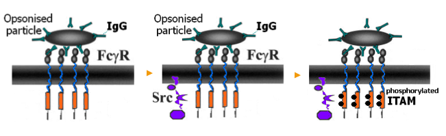
Figure 1: A simple model of the phosphorylation of the ITAM domain on the Fc$\gamma$ receptor during phagocytosis. Adapted from [8].

Fc$\gamma$R contains within its cytoplasmic tail an immunoreceptor tyrosine-based activation motif (ITAM). The association of Fc$\gamma$R with an IgG induces the phosphorylation of two tyrosine residues within the ITAM domain by Src-family kinases. The phosphorylated ITAM domain then recruits Syk kinase, which propagates the signal further to downstream effectors (see Figure 1). In our language, we can describe the initial phases of this cascade as follows:

site f on FcR associates site i on IgG with rate 2.0
site y on FcR gets phosphorylated if site f on FcR is bound
site z on FcR gets phosphorylated if site f on FcR is bound

The first sentence above describes the binding of Fc$\gamma$R to IgG. The second and third sentences describe the phosphorylation of the two tyrosine residues on ITAM (association of a Phosph0() molecule). This is automatically translated by our tool into the SPiM program given in Appendix A. We can then run stochastic simulations on the model given by these sentences.

By using this language and our translation tool, we can build models of different size and complexity, and modify and extend these models with respect to the knowledge in hand on the different sites and interaction capabilities of the Fc$\gamma$R, as well as other biological systems. For example, the model above abstracts away from the role played by the Src kinases in the phosphorylation of the Fc$\gamma$R as depicted in Figure 1. The sentences above can be easily modified and extended to capture this aspect in the model as follows: here, the shaded part demonstrates the modifications with respect to the model given above.

site f on FcR associates site i on IgG with rate 2.0
site y on FcR gets phosphorylated if site $s$ on FcR is bound
site z on FcR gets phosphorylated if site $s$ on FcR is bound
site s on FcR associates site sr on Src if site f on FcR is bound
site s on FcR dissociates site sr on Src

The $\mathsf{SPiM}$ program resulting from automated translation of this model is given in Appendix B. It is important to note that, because FcR has 4 binding sites in the model above, in the $\mathsf{SPiM}$ code resulting from the translation, there are 16 species for FcR, denoting its different possible states. However, in the code given in Appendix A, there are 8 species for FcR denoting its states that result from its 3 binding sites in that model.

5 Discussion

We have introduced a natural language interface for building stochastic $\pi$ calculus models of biological systems. The $\kappa$-calculus [5, 6, 7] and the work on Beta-binders in [11] have been source of inspiration for this language.

In [11], Guerriero et al. give a narrative style interface for the process algebra Beta-binders for a rich biological language. In our language, we build complex events such as phosphorylation and dephosphorylation of sites as instances of basic primitives of association, dissociation and transformation. We give a functional translation algorithm for our translation into stochastic $\pi$ calculus. The conditions that we impose on the models are automatically verified in the implementation of our tool. These conditions should be instrumental for ‘debugging’ purposes while building increasingly large models.

The implicit semantics of our language, which is implemented in the translation algorithm into $\pi$ calculus, can be seen as a translation of a fragment of the $\kappa$ calculus into $\pi$ calculus. Another approach similar to the one in this paper is the work by Laneve et al. in [15], where the authors give an encoding of nano-$\kappa$-calculus in $\mathsf{SPiM}$. In comparison with our algorithm, the encoding in [15] covers a larger part of nano-$\kappa$ by using the $\mathsf{SPiM}$ language as a programming language for implementing a notion of term rewriting, where there is an explicit function for matching. The algorithm gives the different states of a species in the $\mathsf{SPiM}$ encoding with respect to the parameters of that species as in $\kappa$-calculus.

Topics of future work include an exploration of the expressive power of the association, dissociation and transformation primitives with respect to Kohn diagram representation [10] of biological models.

Appendix A

site f on FcR associates site i on IgG with rate 2.0
site y on FcR gets phosphorylated if site f on FcR is bound
site z on FcR gets phosphorylated if site f on FcR is bound

The $\mathsf{SPiM}$ code resulting from the automated translation of this model.

directive sample 10.0
directive plot FcR7(); FcR6();
        FcR5();  FcR4(); FcR3();
        FcR2(); FcR1();
        FcR0(); IgG1(); IgG0();
        Phosph1(); Phosph0()

new fi1@1.0:chan(chan)
new phosphy2@1.0:chan(chan)
new phosphz3@1.0:chan(chan)
new nil@0.0:chan

let FcR0() =
     ( new f@1.0:chan
       !fi1(f)*2.0; FcR1(f) )


and FcR1(f:chan) =
     ( do ?phosphy2(y); FcR4(f,y)
       or ?phosphz3(z); FcR5(f,z) )

and FcR2(y:chan) =
     ( new f@1.0:chan
       !fi1(f)*2.0; FcR4(f,y) )

and FcR3(z:chan) =
     ( new f@1.0:chan
       !fi1(f)*2.0; FcR5(f,z) )

and FcR4(f:chan,y:chan) =
     ( ?phosphz3(z); FcR7(f,y,z) )


and FcR5(f:chan,z:chan) =
     ( ?phosphy2(y); FcR7(f,y,z) )

and FcR6(y:chan,z:chan) =
     ( new f@1.0:chan
       !fi1(f)*2.0; FcR7(f,y,z) )

and FcR7(f:chan,y:chan,z:chan) =
     ()

let IgG0() =
     ( ?fi1(i); IgG1(i) )

and IgG1(i:chan) =
     ()

let Phosph0() =
     ( new phosph@1.0:chan
       do !phosphy2(phosph)*1.0;
            Phosph1(phosph)
       or !phosphz3(phosph)*1.0;
            Phosph1(phosph) )

and Phosph1(phosph:chan) =
     ()


run 1000 of  FcR0()
run 1000 of  IgG0()
run 1000 of  Phosph0()

6 Appendix B

site f on FcR associates site i on IgG with rate 2.0
site y on FcR gets phosphorylated if site $s$ on FcR is bound
site z on FcR gets phosphorylated if site $s$ on FcR is bound
site s on FcR associates site sr on Src if site f on FcR is bound
site s on FcR dissociates site sr on Src

The $\mathsf{SPiM}$ code resulting from the automated translation of this model.

directive sample 10.0
directive plot FcR15();
      FcR14(); FcR13(); FcR12();
      FcR11(); FcR10();
      FcR9(); FcR8(); FcR7();
      FcR6(); FcR5();
      FcR4(); FcR3(); FcR2();
      FcR1(); FcR0();
      IgG1(); IgG0();
      Phosph1(); Phosph0();
      Src1(); Src0()

new fi1@1.0:chan(chan)
new phosphx2@1.0:chan(chan)
new phosphy3@1.0:chan(chan)
new ssr4@1.0:chan(chan)
new nil@0.0:chan


let FcR0() =
 ( new f@1.0:chan
    !fi1(f)*2.0; FcR1(f) )

and FcR1(f:chan) =
 ( new s1@0.50:chan
   !ssr4(s1)*1.0; FcR5(f,s1) )

and FcR2(s1:chan) =
 ( new f@1.0:chan
   do !fi1(f)*2.0; FcR5(f,s1)
   or ?phosphx2(x); FcR8(s1,x)
   or ?phosphy3(y); FcR9(s1,y)
   or !s1; FcR0() or ?s1; FcR0() )

and FcR3(x:chan) =
 ( new f@1.0:chan
   !fi1(f)*2.0; FcR6(f,x) )

and FcR4(y:chan) =
 ( new f@1.0:chan
   !fi1(f)*2.0; FcR7(f,y) )

and FcR5(f:chan,s1:chan) =
 ( do ?phosphx2(x); FcR11(f,s1,x)
   or ?phosphy3(y); FcR12(f,s1,y)
   or !s1; FcR1(f) or ?s1; FcR1(f) )

and FcR6(f:chan,x:chan) =
 ( new s1@0.50:chan
   !ssr4(s1)*1.0; FcR11(f,s1,x) )

and FcR7(f:chan,y:chan) =
 ( new s1@0.50:chan
   !ssr4(s1)*1.0; FcR12(f,s1,y) )

and FcR8(s1:chan,x:chan) =
 ( new f@1.0:chan
   do !fi1(f)*2.0; FcR11(f,s1,x)
   or ?phosphy3(y); FcR14(s1,x,y)
   or !s1; FcR3(x) or ?s1; FcR3(x) )

and FcR9(s1:chan,y:chan) =
 ( new f@1.0:chan
   do !fi1(f)*2.0; FcR12(f,s1,y)
   or ?phosphx2(x); FcR14(s1,x,y)
   or !s1; FcR4(y) or ?s1; FcR4(y) )

and FcR10(x:chan,y:chan) =
 ( new f@1.0:chan
   !fi1(f)*2.0; FcR13(f,x,y) )

and FcR11(f:chan,s1:chan,x:chan) =
 ( do ?phosphy3(y); FcR15(f,s1,x,y)
   or !s1; FcR6(f,x) or ?s1; FcR6(f,x) )

and FcR12(f:chan,s1:chan,y:chan) =
 ( do ?phosphx2(x); FcR15(f,s1,x,y)
   or !s1; FcR7(f,y) or ?s1; FcR7(f,y) )

and FcR13(f:chan,x:chan,y:chan) =
 ( new s1@0.50:chan
   !ssr4(s1)*1.0; FcR15(f,s1,x,y) )

and FcR14(s1:chan,x:chan,y:chan) =
 ( new f@1.0:chan
   do !fi1(f)*2.0; FcR15(f,s1,x,y)
   or !s1; FcR10(x,y) or ?s1; FcR10(x,y) )

and FcR15(f:chan,s1:chan,x:chan,y:chan) =
 ( do !s1; FcR13(f,x,y) or ?s1; FcR13(f,x,y) )


 let IgG0() =
   ( ?fi1(i); IgG1(i) )

 and IgG1(i:chan) =
   ()


 let Phosph0() =
   ( new phosph@1.0:chan
     do !phosphx2(phosph)*1.0;
     Phosph1(phosph)
     or !phosphy3(phosph)*1.0;
     Phosph1(phosph) )

 and Phosph1(phosph:chan) =
   ()


 let Src0() =
   ( ?ssr4(sr1); Src1(sr1) )

 and Src1(sr1:chan) =
   ( do !sr1; Src0() or ?sr1; Src0() )


 (* run  1000 of ... *)

References

- [1] L. Cardelli, E. Caron, P. Gardner, O. Kahramanoğulları, and A. Phillips. A process model of actin polymerisation. In FBTC’08, volume 229 of ENTCS, pages 127–144. Elsevier, 2008.
- [2] L. Cardelli, E. Caron, P. Gardner, O. Kahramanoğulları, and A. Phillips. A process model of Rho GTP-binding proteins. Theoretical Computer Science, 410/33-34:3166–3185, 2009.
- [3] L. Cardelli and G. Zavattaro. On the computational power of biochemistry. In AB’08, volume 5147 of LNCS, pages 65–80. Springer, 2008.
- [4] C. Cougoule, S. Hoshino, A. Dart, J. Lim, and E. Caron. Dissociation of recruitment and activation of the small G-protein Rac during Fc gamma receptor-mediated phagocytosis. J. Bio. Chem., 281:8756–8764, 2006.
- [5] V. Danos, J. Feret, W. Fontana, R. Harmer, and J. Krivine. Rule-based modelling of cellular signalling. In CONCUR’07, volume 4703 of LNCS, pages 17–41. Springer, 2007.
- [6] V. Danos, J. Feret, W. Fontana, R. Harmer, and J. Krivine. Rule-based modelling, symmetries, refinements. In FMSB’08, volume 5054 of LNCS, pages 103–122. Springer, 2008.
- [7] V. Danos, J. Feret, W. Fontana, and J. Krivine. Abstract interpretation of cellular signalling networks. In VMCAI’08, volume 4905 of LNBI, pages 83–97. Springer, 2008.
- [8] E. Garcia-Garcia and C. Rosales. Signal transduction during Fc receptor-mediated phagocytosis. Journal of Leukocyte Biology, 72:1092–1108, 2002.
- [9] M. Heiner, D. Gilbert, and R. Donaldson. Petri nets for systems and synthetic biology. In SFM’08, volume 5016 of LNCS, pages 215–264. Springer, 2008.
- [10] K. W. Kohn, M. I. Aladjem, S. Kim, J. N. Weinstein, and Y. Pommier. Depicting combinatorial complexity with the molecular interaction map notation. Molecular Systems Biology, 2:51, 2006.
- [11] C. Priami M. L. Guerriero, J. K. Heath. An automated translation from a narrative language for biological modelling into process algebra. In CMSB’07, volume 4695 of LNCS, pages 136–151. Springer, 2007.
- [12] R. Milner. Communication and Mobile Systems: the -calculus. Cambridge University Press, 1999.
- [13] A. Phillips and L. Cardelli. Efficient, correct simulation of biological processes in stochastic Pi-calculus. In CMSB’07, volume 4695 of LNBI. Springer, 2007.
- [14] A. Phillips, L. Cardelli, and G. Castagna. A graphical representation for biological processes in the stochastic pi-calculus. In Transactions on Computational Systems Biology VII, volume 4230 of LNCS, pages 123–152. Springer, 2006.
- [15] S. Pradalier, C. Laneve, and G. Zavattaro. From biochemistry to stochastic processes. In QALP’09, ENTCS. Elsevier, 2009. to appear.
- [16] C. Priami, A. Regev, E. Shapiro, and W. Silverman. Application of a stochastic name-passing calculus to representation and simulation of molecular processes. Information Processing Letters, 80:25–31, 2001.
- [17] A. Regev and E. Shapiro. Cellular abstractions: Cells as computation. Nature, 419:343, 2002.
- [18] J. A. Swanson and A. D. Hoppe. The coordination of signaling during Fc receptor-mediated phagocytosis. Journal of Leukocyte Biology, 76:1093–1103, 2004.
- [19] A. Tiwari, C. Talcott, M. Knapp, P. Lincoln, and K. Laderoute. Analyzing pathways using sat-based approaches. In Gerhard Goos, Juris Hartmanis, and Jan van Leeuwen, editors, Second International Conference, Algebraic Biology 2007, volume 4545 of LNCS, pages 155–169. Springer, 2007.