Beyond power laws: Universality in the average avalanche shape

We report the measurement of multivariable scaling functions for the temporal average shape of Barkhausen noise avalanches, and show that they are consistent with the predictions of simple mean-field theories. We bypass the confounding factors of time-retarded interactions (eddy currents) by measuring thin permalloy films, and bypass thresholding effects and amplifier distortions by applying Wiener deconvolution. We find experimental shapes that are approximately symmetric, and track the evolution of the scaling function. We solve a mean-field theory for the magnetization dynamics and calculate the form of the scaling function in the presence of a demagnetizing field and a finite field ramp-rate, yielding quantitative agreement with the experiment.

The study of critical phenomena and universal power laws has been one of the central advances in statistical mechanics of the second half of the last century, in explaining traditional thermodynamic critical points wilson75 , avalanche behavior near depinning transitions fisher98 ; doussal09 , and a wide variety of other phenomena sethna01 . Scaling, universality, and the renormalization group claim to predict all behavior at long length and time scales asymptotically close to critical points. In most cases, the comparison between theory and experiments has been limited to the evaluation of the critical exponents of the power law distributions predicted at criticality. An excellent playground of scaling phenomena is provided by systems exhibiting crackling noise, such as the Barkhausen effect in ferromagnetic materials durin06 . Here we focus on the average functional form of the noise emitted by avalanches — the temporal average avalanche shape sethna01 .

This avalanche shape has been measured for earthquakes mehta02 and for dislocation avalanches in plastically deformed metals chrzan94 ; laurson06 , but the primary experimental and theoretical focus has always been Barkhausen avalanches in magnetic systems kuntz00 ; durin02 ; mehta02 ; durin06 ; colaiori08 . Theory and experiment agreed well for avalanche sizes and durations, but the strikingly asymmetric shapes found experimentally in ribbons durin02 , disagreed sharply with the theoretical predictions, for which the asymmetry in the scaling shapes under time reversal was at most very small mehta02 ; sethna01 . (We note that the relevant models are not microscopically time-reversal invariant; temporal symmetry is thus emergent). Doubts about universality sethna01 were resolved when eddy currents were shown to be responsible for the asymmetry, at least on short time scales zapperi05 , but the exact form of the asymptotic universal scaling function of the Barkhausen avalanche shape still remained elusive.

In this paper, we report an experimental study of Barkhausen noise in permalloy thin films, where a careful study of the average avalanche shapes leads to symmetric shapes, undistorted by eddy currents (which are suppressed by the sample geometry). We provide a quantitative explanation of the experimental results by solving exactly the mean-field theories for two general models of magnetic reversal: a domain wall dynamics model alessandro90 and the random-field Ising model sethna93 . The two mean-field theories are shown to be equivalent, and allow us to compute the average avalanche temporal shape as a function of typical experimental control parameters such as the field rate and the demagnetizing factor.

The relevant statistical information encoded in the Barkhausen noise could in principle be derived from the joint two-point time-velocity distribution $G_{c,k}(V,t;V^{\prime},t+\Delta)$, yielding the conditional probability that the noise at time $t+\Delta$ is equal to $V^{\prime}$ if it was equal to $V$ at time $t$. Here $c$ is the external field rate and $k$ the demagnetizing factor. The standard avalanche distributions can be derived from this parent distribution, e.g. the duration distribution is given by

$$P(T)=-\int_{0}^{\infty}dV\partial_{\Delta}G_{c,k}(0^{+},t;V,t+\Delta)|_{\Delta=T}.$$ (1)

The renormalization group makes use of an emergent scale invariance for Barkhausen noise. Here, the two-point time-velocity distribution, when coarse-grained in time by a factor $b$ and rescaled downward in velocity by a factor $b^{x}$, rescales at long durations to itself:

$$G_{c,k}(V,t;V^{\prime},t+\Delta)=b^{-2x}G_{\bar{c},\bar{k}}(V/b^{x},t/b\,;\,V^{\prime}/b^{x},(t+\Delta)/b),$$ (2)

where $\bar{c}=b^{y}c$ is the rescaled field rate, $\bar{k}=b^{w}k$ the rescaled demagnetizing factor and $x,y,w$ are universal scaling exponents. Repeating $n$ rescalings until $\Delta/b^{n}=1$ leads to a universal scaling form

$$G_{c,k}(V,t;V^{\prime},t+\Delta)=\Delta^{-2x}{\cal G}(\Delta^{-x}V,\Delta^{-x}V^{\prime},\Delta^{y}c/c_{0},\Delta^{w}k/k_{0}).$$ (3)

where ${\cal G}$ is a universal multivariable scaling function and $c_{0}$ and $k_{0}$ are the small scale values of the field rate and demagnetizing factor, respectively.

Universal scale invariant forms can then be derived for all statistical quantities of interest including the temporal average shape. For avalanches of duration $T$, the average shape is defined as the average velocity for avalanches that begin and end at $V=0$ in a duration $T$. It has an associated universal scaling form,

$$\langle V_{c,k}(\Delta|T)\rangle = \int dV^{\prime}V^{\prime}G_{c,k}(0^{+},0;V^{\prime},\Delta)G_{c.k}(V^{\prime},\Delta;0,T)/\int dV^{\prime}G_{c,k}(0^{+},0;V^{\prime},\Delta)G_{c,k}(V^{\prime},\Delta;0,T)$$ (4)

$$= T^{x}{\cal V}(\Delta/T,(k/k_{0})T^{w},c/c_{0}T^{y}),$$

where ${\cal V}(\lambda,K,C)$ is a universal scaling function, dependent on the rescaled time $\lambda\equiv\Delta/T$, the rescaled demagnetizing factor $K\equiv(k/k_{0})T^{w}$, and the driving field $C\equiv(c/c_{0})T^{y}$. It is universal in the sense that in the scaling regime does not depend on microscopic features of the material, so long as the system is at a critical point.

We record the Barkhausen noise by a standard inductive technique on a 1 $\mu$m thick permalloy film, with polycrystalline structure (see methods section for details on the measurement and on sample preparation). The Barkhausen noise is composed by a series of intermittent pulses, due to avalanches in the magnetization, combined with background instrumental noise. In most crackling noise phenomena, avalanches are usually identified by setting a threshold above the background noise $V_{\mathrm{th}}$. This method works well if the signal to noise ratio is high, but can induce spurious effects otherwise laurson09 . Our thin films have a correspondingly weak signal, making the $V_{\rm th}$ inappropriate. In addition, the measurement apparatus has a response function that distorts the original pulses. We instead extract the pulses using Wiener deconvolution book-nr , which optimally filters the background noise and bypasses the use of thresholds (see Fig. S1).

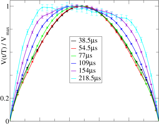
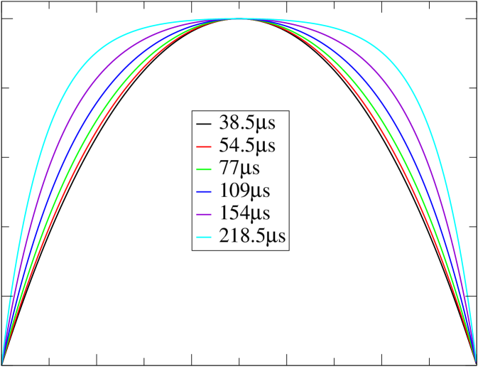
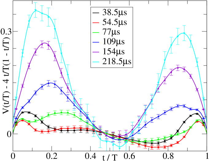
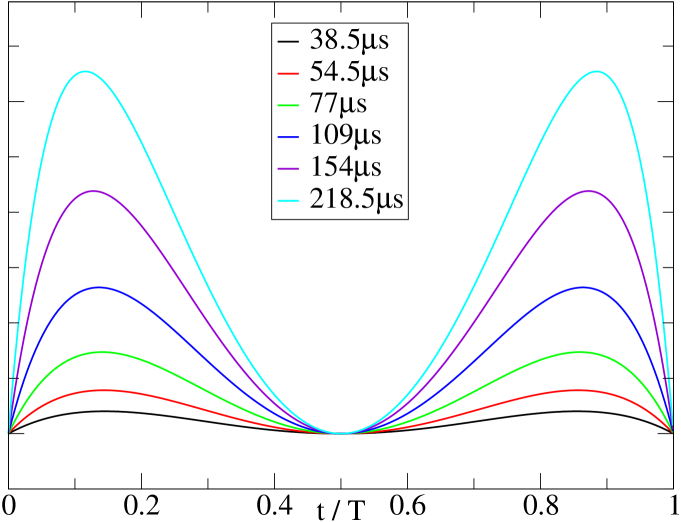
Figure S3: Experiment and theory: Average shapes and scaling. (a) The temporal average avalanche shape for different avalanche durations $T$, rescaled to unit height and duration. The 218.5 $\mu$s curve, for example, represents the average over $658$ avalanches, with durations between 181 $\mu$s and 256 $\mu$s, binned in $50$ equal time intervals, each of size $4.37~{}\mu$s . Notice the symmetric, parabolic shape for short durations, and the flattening for longer durations. The small residual asymmetry remaining is plausibly attributable to amplifier-induced distortions that were not possible to correct for. The impulse response functions of the individual instruments (amplifier, low-pass filter and sensing coils) were measured subsequent to taking the data, and used to deconvolve the resulting signal (cf. Supplementary Information). (b) Mean-field calculation for the average shape including a demagnetizing factor $k$ as in Eq. 5. The shape is an inverted parabola, $4t/T(1-t/T)$ for short durations and flattens at long durations. Here, $k$ is $0.05~{}\mu$s^-1, slightly different from the value used in Fig. S2. This difference is expected since our analytical form is only available for $c=0$; simulations at $c,k$ given in the insets of Fig. S2a and b respectively, yields good, albeit noisy, agreement with experiment. (c,d) Deviations from the inverted parabola. Note the quantitative agreement between experiment and theory.

The universality class of the Barkhausen noise in a sample is usually identified by measuring the voltage distribution, the power spectrum and the distributions of avalanche sizes $S$ and durations $T$ durin00 . The present experiments display characteristic features of the mean-field universality class: we observe a field-rate dependence of the voltage distribution and of the avalanche size and duration distributions that is in excellent agreement with mean-field predictions (see Fig. S2(a), (b) and (d), noting in each case the three variable scaling implied by the field rate and demagnetizing factor). Furthermore, the power spectrum and the conditional average size of an avalanche of duration $T$ are rate independent and consistent with mean-field predictions (see Fig. S2(c)). Finally, we focus on the measurement of the average avalanche temporal shape, considering all the avalanches of a given duration $T$ and averaging the voltage signal at each time step $t$. (In practice, we average the avalanches using duration bins centered at $T$ and with geometrically increasing sizes). Fig. S3(a) shows the resulting nearly symmetric temporal average avalanche shape, which starts out parabolic and then flattens as the duration of the avalanche increases (cf. Fig. S3(c)).

It has been argued that dipolar magnetic fields are sufficiently long-ranged that mean-field theory should be quantitatively applicable in three dimensional samples zapperi98 . Similar considerations apply to many of the systems exhibiting crackling noise, such as dislocation-mediated plasticity zaiser06 and earthquakes fisher97 where long-range interactions are provided by elastic strains. Our films are thinner than polycrystalline ribbons known to exhibit mean-field behavior durin00 , but thicker than previously studied 2D films kimnat . The classic mean-field theory for domain wall depinning is the single-degree of freedom ABBM model alessandro90 , which treats the domain wall as a rigid object at position $X(t)$, advancing in a random pinning field statistically chosen as a random walk in $X$,

$$\Gamma\frac{dX}{dt}=ct-kX+W(X),$$ (5)

with $\langle W(X)\rangle=0$ and $\langle W(X)W(X^{\prime})\rangle=|X-X^{\prime}|$ (Brownian noise) and where $\Gamma$ is the damping coefficient. The ABBM model predicts that the avalanche size and duration distributions decay as power laws with rate dependent exponents colaiori08 . The exact form of the scaling functions for these distributions, including the cutoff to the power law behavior, can be computed in the limit $c=0$ colaiori08 . To compare with experiments for $c>0$, we resort to numerical integration of Eq. 5, obtaining close agreement, as displayed in Fig. S2.

The average avalanche shape in the ABBM model has not been extensively explored numerically, but an approximate analytical calculation colaiori04 ; colaiori08 gave a lobe of a sinusoid ${\cal V}(\lambda)\simeq\sin(\pi\lambda)$. In that calculation, the approximation $\langle V(X(t),T)\rangle\simeq V(\langle X(t)\rangle,T)\rangle$ was made. (That is, the fluctuations in the growth of the avalanche size with time were neglected, leading to a slight distortion of the predicted temporal average avalanche shape.) We avoid this approximation by using a transformation due to Bertotti bertottibook to a time-dependent noise with a variance proportional to the avalanche velocity $V$

$$\frac{dV}{dt}=c-kV+\sqrt{2V}\xi(t),$$ (6)

which can be solved in the Stratonovich interpretation in the limit $c=0$, $k=0$. After defining a new variable $Y=V^{1/2}$, we have a stochastic equation that we may solve explicitly. Utilizing the resulting probability for the first-return to the origin, we calculate the temporal shape baldassarri03 ; colaiori08  (cf. Supplementary Information) :

$$\langle V_{c=0,k=0}(t|T)\rangle=\frac{1}{8}t\left(1-\frac{t}{T}\right),$$ (7)

where in the future we will use $t$ instead of $\Delta$ to denote the time elapsed from the beginning of the avalanche. We have numerically verified that the average shape is indeed an inverted parabola (and not the lobe of a sine wave colaiori08 ).

Interestingly, an inverted parabola was reported kuntz00 ; mehta02 in numerical studies of the (nucleated) random-field Ising model in the mean-field limit (the ‘shell’ model) sethna93 . Front depinning and nucleated transitions have different upper critical dimension and different short-range critical exponents, and it was conceivable that their mean-field theories had different average shapes, albeit sharing critical exponents.

Upon closer examination, these two models are the same in the continuum limit. The shell model has a set of interacting spins $M_{i}=\pm 1$ with random fields $h_{i}$ distributed by a Gaussian, interacting with a strength $J/N$ with all other spins; each spin flips when the net field it feels, $h_{i}+H(t)+J/N\sum_{j}S_{j}$ is positive. Here, $H(t)=H_{0}+ct$ is the external field, increasing with rate $c$, and the spin feels the magnetization $M=(1/N)\sum_{j}S_{j}$ both through the infinite-range coupling $J/N$ and the demagnetizing factor $k$. A shell-model avalanche proceeds in parallel, with a shell of $V_{n}$ unstable spins flipping at the $n-$th time-step, then triggering a new set of spins $V_{n+1}$ to flip:

$$V_{n+1}=P(2JV_{n}),$$ (8)

where $P$ is the Poisson distribution for the set of spins $V_{n+1}$ to be included in the range $\{f,f+2JV_{n}\}$. For large $V$, we may approximate the Poisson distribution as a Gaussian $P(V)=V+\sqrt{V}\xi$, leading to $V_{n+1}-V_{n}\simeq-\tilde{k}V_{n}+\sqrt{JV_{n}}\xi(t)$ which is clearly a discretized version of Eq. 6, where $\tilde{k}=1-2J$ is the distance to the critical threshold. This equivalence, in retrospect, provides an alternative explanation for the origin of Brownian noise statistics for the ABBM domain wall potential zapperi98 .

Finally, we consider the effects of the two main physical perturbations, the driving field $c$ and the demagnetizing factor $k$. The transformed Eq. 6 now takes the form

$$\frac{dY(t)}{dt}=\frac{c}{Y}-kY(t)+\frac{1}{\sqrt{2}}\xi(t).$$ (9)

Under rescaling $\sqrt{V}=Y\rightarrow b^{-x/2}Y$, $t\rightarrow t/b$ and for uncorrelated Gaussian white noise we have $\xi\rightarrow b^{1/2}\xi$. By balancing the noise with the left-hand side, we find $x=1$; thus the driving field is marginal ($y=0$), and the demagnetizing factor is relevant with scaling dimension $w=1$. The demagnetizing factor $k$ sets the characteristic maximum of the avalanche size and duration. The two-point probability function in the case $c=0$ can be found exactly vankampenbook and the functional form of the resulting shape is,

$$\langle V_{c=0,k}(t|T)\rangle = \frac{1}{2k}\frac{(e^{2k(T-t)}-1)(e^{2kt}-1)}{e^{2kT}-1},$$ (10)

and hence the scaling function is

$${\cal V}(\lambda,K,0)=\frac{1}{K}\frac{(e^{K(1-\lambda)}-1)(e^{K\lambda}-1)}{e^{K}-1}.$$ (11)

Intuitively, the form of the scaling function leads to a flattening of the average shape at long times because $k$ acts to cap the velocities. As it can be seen in Fig. S3, this behavior is verified by our experiments.

The effect of the driving field $c$, a marginal field at mean-field, can be calculated exactly at $k=0$ using a result from Ref. bray00 : for an absorbing boundary condition at $V=0$, the two-points probability function for the Brownian motion in a logarithmic potential is $G_{c,k=0}(V,t;\epsilon,0)=\frac{4}{\Gamma[1+\nu]}(4t)^{-(1+\nu)}\epsilon^{2\nu}Ve^{-V^{2}/(4t)}(1+O(\epsilon^{2}))$, where $\nu=(1-c)/2$. Using this expression, the scaling form is reduced in magnitude but remains parabolic, with ${\cal V}(\lambda,0,C)=(1/8)(1+C)\lambda(1-\lambda)$.

In conclusion, we have used multivariable universal scaling functions to study average avalanche temporal shapes in Barkhausen noise. By analyzing thin films, we have bypassed the eddy current effects that have long frustrated complete comparison between theory and experiment. We unify the two rival mean field theories, calculate both the mean-field scaling function for the temporal average shape and the effects of the demagnetizing factor and the field rate. By utilizing optimal Wiener filtering techniques we allow an unbiased capturing of the shapes, allowing us to report almost symmetric shapes, yielding excellent agreement with our theoretical predictions.

Methods

Sample preparation and experimental measurements

A 1 $\mu$m thick ferromagnetic film with nominal composition Ni₈₁Fe₁₉ (permalloy) is deposited by magnetron sputtering from a commercial target, on a glass substrate covered by a 2 nm thick Ta buffer layer. The deposition is performed with the substrate moving at constant speed through the plasma in order to improve the film uniformity, with the following parameters: base vacuum of $10^{-7}$ Torr, deposition pressure of 5.2 mTorr (99.99 % pure Ar at 20 SCCM constant flow), and 65 W RF power. The deposition rate of 0.28 nm/s is calibrated with x-ray diffraction, which also confirms the polycrystalline character of the film. Quasi-static magnetization curves obtained with a vibrating sample magnetometer indicate isotropic in-plane magnetic properties with an out-of-plane anisotropy contribution, a behavior related to the stress stored in the film, and to the columnar microstructure  hubertbook ; viegas01 ; santi06 .

Barkhausen noise time series are obtained using the inductive technique in an open magnetic circuit. The sample has dimensions 10 mm $\times$ 4 mm. Sample and pickup coils are inserted in a long solenoid with compensation for the effects of the border. The sample is driven by a triangular driving magnetic field with amplitude high enough to saturate the film ($\pm$ 15 kA/m). The driving field frequency is varied in the range 0.05 Hz-0.4 Hz. Barkhausen noise is detected by a 400 turn sensing coil (3.5 mm long, 4.5 mm wide, 1.25 MHz resonance frequency) wound around the central part of sample. A second pickup coil, with the same cross section and number of turns, is adapted in order to compensate the signal induced by the magnetizing field. The Barkhausen signal is then amplified and filtered with a 100 kHz low-pass filter, and finally acquired data at 0.2 and 4 MSamples/s. The data at different rates are statistically very similar after Wiener filtering (spurious peaks are present in the high frequency regime of the spectrum, independently of the rate), with very small differences at short durations and small voltages. Wiener filtering is practically more efficient at large rates, for uncorrelated noise, but the noise amplitude remains larger than at low rates. Thus, the optimal use of this filter depends on the observables studied: For the distributions in Fig. S2, in order to gain more accuracy at short durations and small avalanches sizes by reducing the noise level, the low rate is used; For the average temporal shapes, in Fig. S3, being more important to capture variations of the signal at small timescales by a more accurate Wiener filter, the large rate is used. The time series is acquired just around the central part of the hysteresis loop near the coercive field, where the domain wall motion is the main magnetization mechanism  bertottibook ; bohn2007 . By using a thin film, we have removed the confounding effects of eddy currents, whose time scale zapperi05 for the present sample is estimated to be $T_{p}\sim 0.04~{}\mu$s, much smaller than the avalanche durations studied.

Data analysis

To address the low signal from the thin film, we analyze the data by using Wiener deconvolution book-nr . The form of the output signal is assumed to be of the form $V_{out}(t)=(h\star(V+n))(t)$ where $h(t)$ denotes the impulse response function, $V(t)$ the original microscopic signal, and $n(t)$ the background noise. Given an estimated impulse response Fourier series $\tilde{h}(f)$, an estimated deconvolved noise power spectrum $|\tilde{n}(f)|^{2}$ and a theoretically expected frequency spectrum for the deconvolved signal $|\tilde{v}(f)|^{2}$, the filtered data $V(t)$ is the inverse Fourier transform of

$$\tilde{V}(f)=\frac{\tilde{V}_{out}(f)}{\tilde{h}(f)}\frac{|\tilde{v}(f)|^{2}}{|\tilde{n}(f)|^{2}+|\tilde{v}(f)|^{2}}.$$ (12)

Here, the impulse function is estimated by measuring the impulse response of the individual instruments composing the apparatus. We note that if the signal has a high resolution, a detailed knowledge of the impulse response function is needed to remove the effect of the instrument. As a signal function, we use a power fit $|\tilde{v}(f)|^{2}\sim f^{-\gamma}$ (see also Supplementary Information). To estimate the noise contribution $|\tilde{n}(f)|^{2}$, we measure the power spectrum of the instrumental noise, recorded without the material, maximizing over several runs. The Wiener deconvolution, shown in Fig. S1 and in the inset of Fig S2c, smoothens the signal, and removes spurious high frequency oscillations, due to the amplifier and filters used in the experiments. Importantly, this procedure also allows us to avoid the use of thresholds for defining the temporal extent of the avalanches, improving our estimates for both the scaling exponents and the average avalanche shapes.

Supplementary Information is linked to the online version of the paper.

Author Contributions

F.B., G.D., and R.L.S. were responsible for the experiments. F.B. had primary responsibility for the sample production and characterization, the experimental setup, and the experimental data acquisition. R.L.S. was responsible for the design of the sample production and characterization methods and supervised the experimental design and execution. G.D. inspired the project, guided the development of the experimental design, and both supervised and participated in the data acquisition. S.P., S.Z., and J.P.S. were responsible for the implementation of the Wiener filtering methods. The data analysis, partly based on software by S.Z., was adapted by all three, and then tested, refined, and executed by S.P. F.B., G.D., and R.L.S. provided key input into the interpretation and presentation of the data. S.P. was responsible for the theoretical analysis of the avalanche shapes and for the simulations. S.P. wrote the original text of the manuscript; all authors contributed to refining and focusing the text.

Author information

The authors declare no competing financial interests. Correspondence and requests for materials should be addressed to S.P. (stefan@ccmr.cornell.edu).

Figure Legends

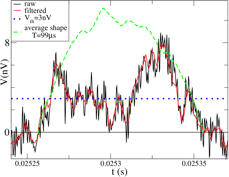
Figure S1: Extracting average shapes from noisy data by Wiener deconvolution. Time-series data (jagged line) is traditionally separated into avalanches using a threshold $V_{\mathrm{th}}$ set above the instrumental noise (dotted blue line) – here breaking one avalanche into a few pieces. We instead do an optimal Wiener deconvolution (smoothed red curve, see text), allowing the use of a zero threshold (solid black line) which avoids distortions of the average shape and also gives more decades of size and duration scaling. Averaging over all avalanches with this duration gives us $\langle V(t,T)\rangle$ (dashed green curve).

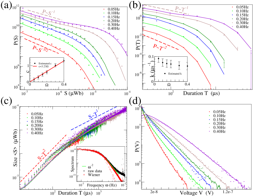
Figure S2: Multivariable scaling; experiment vs. mean-field theory. In each main graph, the symbols represent data taken at various sweep frequencies $\Omega$ for the external field. The lines represent mean-field predictions extracted from ABBM simulations (cf. Eq. 6) with parameters $c$ and $k$ shown in the insets of (a) and (b), taking similar number of samples with the experiment; the sweep rate $c\propto\Omega$ as predicted, and the weak dependence of the demagnetizing factor $k$ can plausibly be attributed to changing experimental conditions. The distribution of avalanche sizes and durations shown in (a) and (b) depend on three variables (demagnetizing factor, sweep frequency, and $S$ or $T$); no analytical form is available, but the agreement with the mean-field simulations is excellent. Avalanches of longer duration merge when ramped at a finite rate, leading to unusual rate-dependent critical exponents in mean-field theory; the smaller avalanches have $P\sim S^{-\tau}$ with $\tau=3/2-c/2$, while the briefer ones have $P\sim T^{-\alpha}$ with $\alpha=2-c$. (Vertical scales are shifted for clarity; vertical units are arbitrary.) The limiting values of $c=0$ and $c=1$ (corresponding to $\Omega=0.3$) are shown. The mean avalanche size versus duration is shown in (c); for avalanches below the demagetization cutoff $\langle S\rangle\sim T^{2}$, while above the demagnetization cutoff $\langle S\rangle\sim T$ is observed, as expected. Power-law behavior of avalanche sizes versus durations has been observed before in experiments on systems with short-range interactions, but not before on materials believed to belong to the long-range or mean-field universality class durin06 (presumably because of eddy currents). The observed systematic vertical shift with rate of the experimental curves is due to the presence of instrumental noise, not included in the simulations. The inset shows the power spectrum for $\Omega=0.05$ Hz, which has a behavior consistent with $\omega^{-2}$, as predicted by mean-field theory. Finally, in (d) the the voltage probability distribution is consistent with the mean-field prediction $P(V|k,c)\propto V^{c-1}\exp{(-kV)}$, another three-variable scaling form. The observed deviations at small voltages are due to the presence of instrumental noise, being approximately gaussian with $\sigma\approx 18nV$.

Supplementary Information

Beyond power laws: Universality in the average avalanche shape
Stefanos Papanikolaou, Felipe Bohn, Rubem Luis Sommer, Gianfranco Durin,

Stefano Zapperi, and James P. Sethna

In this supplementary information, we

1. Explain in detail how we implemented the optimal Wiener filtering to extract the magnetic avalanche sizes, durations, and temporal shapes from a noisy Barkhausen signal. We show that our methods not only allow for extraction of avalanche shapes, but provide more faithful extraction of avalanche sizes, durations, and velocities from the signal, by comparing filtered and unfiltered analyses both of experiments and of simulations with added noise.

2. Further characterize our films, and discuss issues involved in the 3D-2D crossover, expected in the study of thinner films.

3. Explain the theoretical mapping between the two discussed mean-field theories and describe the approximation made in the previous average shape calculation (which gave a sine scaling function rather than an inverted parabola). In order to demonstrate the technique, we show in detail how to calculate the average shape for $k=c=0$.

.1 Optimal Wiener filtering for extracting Barkhausen avalanches

In this publication we focus on thin magnetic films to avoid the complexities of eddy currents found in ribbons. Because of the reduced thickness, the induced signal is significantly smaller, substantially decreasing the signal-to-noise ratio. The larger number of turns of pick-up coil compensates for the reduced voltage, but also introduces spurious background effects, mainly in the high frequency regime of the spectrum. Such effects clearly demand a more sophisticated extraction of the signal from the noise. We found that the most effective results are obtained by applying an optimal Wiener filter, using independent measurements of the spectral properties of the background noise.

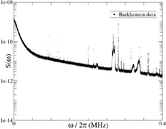
Figure S4: The average power spectrum of the signal. The power spectrum at high frequencies, averaged over 200 runs, is dominated by background noise effects which alter the scaling behavior at intermediate sizes and durations.

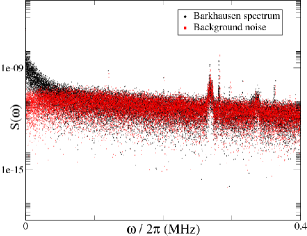
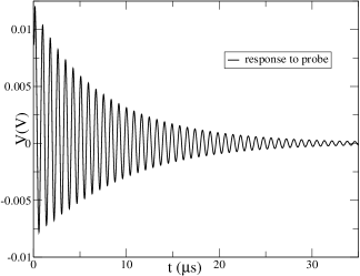
Figure S5: The power spectrum of the instrumental noise after one sweep and the impulse response. The black points in (a) are the power spectrum of one Barkhausen run, out of 200 total used in this paper, deconvolved with the function shown in (b), based on the measured impulse response function for the instrument. The red points in (a) denote the background deconvolved noise spectrum, which (after deconvolution) resembles white noise at low frequencies. The instrumental response in (b) is composed of a low-pass filter response, which is a pure exponential decay and a sensing coil response, which amounts to an oscillatory exponential decay.

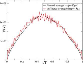
Figure S6: The effect of instrumental noise on the average shapes. The effect of the background noise oscillations on the form of the average shapes is easily observed in the individual avalanches (Fig. 1 in the main text), and dramatic in the average avalanche shapes for fixed (non-binned) durations (above). After filtering, the oscillations are reduced significantly.

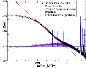
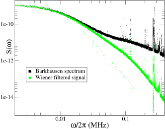
Figure S7: The power spectrum and Wiener deconvolution. (a) The black squares denote the power spectrum of 200 Barkhausen runs for the rate 0.05Hz, deconvolved with the impulse response function of Fig. S5(b). The red curve is a power law fit to the scaling regime of the averaged signal, used in the Wiener deconvolution method. The purple circles denote the average of the background noise spectrum, deconvolved in the same way as the signal, over 200 independent measurements. Finally, the blue curve denotes the estimated noise spectrum, used in the Wiener deconvolution method, which is composed of a white-noise component located at the average amplitude of the background spectrum in the low-frequency regime, and the spurious isolated peaks at high frequencies. Since the positions of the spurious peaks move from run to run, we include them in the noise-estimate whenever the background-noise spectrum of a single run has larger than $3\sigma_{n}$, where $\sigma_{n}$ is the variance of the noise. The form of the signal is plagued with high frequency features that come from artificial background noise elements. (b) After the Wiener deconvolution, the resulting filtered signal’s spectrum averaged over all runs (green diamonds) reduces significantly the distorted features, recovering a large part of the scaling behavior, which is consistent with the mean-field prediction ($S(\omega)\sim\omega^{-2}$).

Optimal Wiener filtering is performed in Fourier space, using the available information about the spectral properties of the signal and the background noise. The signal is predominant in the low-frequency portion of the spectrum where, in general, it shows a power law behavior at intermediate frequencies, going to a constant at low frequencies. Since we are interested in filtering the high-frequency regime of the spectrum, we are very careful about estimating the expected signal $S(\omega)$ at the intermediate frequencies, where scaling takes place. For this purpose, we use a power law fitting function $S(\omega)\sim\omega^{-\gamma}$ for our expected signal (cf. Fig. S7(a)). In this way, the very low frequency regime remains practically unfiltered (since the spectrum intensity of the signal is much larger than that of the noise (cf. Fig. S5(a), S7(a)). The background noise, after deconvolving the instrumental response (cf. Fig. S5(a), S5(b)), is white at low frequencies (cf. Fig. S5(a) and S7(a)). The high-frequency portion of the signal and noise are affected by nonlinear amplifier artifacts (cf. Fig. S5(b)), which produce a series of resonance peaks (cf. Fig. S4, S5(a)). Their effects on the time signal are spurious oscillations which persist also in the average avalanche shape, as seen in Fig. S6. We use this information to set our estimate for the noise spectrum as a sum of two components: i) a white-noise component, being the mean of the Gaussian noise ($\sim 10^{-11}V^{2}Hz^{-1}$), shown in Fig. S7(a). ii) Spurious peaks in the spectrum, with amplitudes larger than three times the white noise’s variance, that are observed to contaminate the signal at high-frequencies. Since these noise peaks are quite sharp and slightly shift from run to run, we use the maximum of these $3\sigma$ events over our 200 independent magnetic field sweeps as our estimated noise spectrum (blue curve in Fig. S7(a)).

With this information on the instrumental noise and on the signal, we apply Eq. 12 of the main text to the FFT of the time signal (cf. S7(a)), and perform the inverse FFT to get the filtered time signal (cf. S7(b)). The average avalanche shapes now appear smooth (see Fig. 2 in the main text).

We test our optimal Wiener filtering by studying its effects on avalanche sizes, durations, and voltages in Fig. S8. We find that the method appears to have significant advantages over both analyzing the unfiltered data and the alternative method of thresholding for extracting smaller avalanches from data (Fig. S8(a) and (c))). We also compare to simulated data (cf. Eq. 6 of the main text) – we add Gaussian noise to match that of the experiment after deconvolution, and then we convolve with the experimentally measured impulse function, to test for potential systematic errors due to the Wiener filtering. We find that the smaller and shorter avalanches and the low voltages (below the noise) are indeed distorted by the process, but that the recovery of large avalanches is significantly enhanced by the Wiener filtering process.

We also use simulated data to explore possible systematic effects on the average avalanche shapes. After adding the noise and convolving with the impulse response function of Fig. S5(b), the average shape develops a significant asymmetry that resembles the one seen in the experiments, shown in Fig. S9. After filtering, this asymmetry disappears completely, since in this case we know the form of the impulse response exactly. In the case of the actual experimental shapes (cf. Fig. 2 of the main text), even though filtering reduces the present small asymmetry, it does not disappear completely, presumably because the true impulse function involves non-linear effects that are hard to identify and correct for. Also, note that the noisy signal includes a systematic correction near the edges of the shape ($t\rightarrow 0$ and $t\rightarrow T$), due to the presence of background noise.

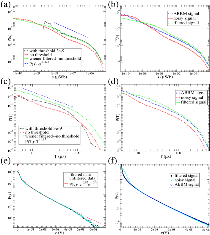
Figure S8: Optimal Wiener filtering effects, tested on experimental data and simulations with added noise. For each pair, the left panel is experiment and the right panel is simulated ABBM mean-field data with $k=0.08$, $c=0.15$, and added noise roughly matching that of the experiment (at rate 0.05 Hz), after deconvolution. (a) and (b) show the avalanche size distributions; (c) and (d) show avalanche duration distributions, and (e) and (f) show voltage distributions. For the experimental size and duration distributions (a) and (c), the optimal Wiener filtering (green) appears to allow the extraction of almost one decade more than either the raw data (red) or data analyzed with the noise threshold depicted in Fig. 1 of the main text. The theoretical size and duration distributions (b) and (d) show the true ABBM distributions (black), the distributions analyzed with added noise (red), and the optimally filtered simulations (green). Here we see that the filtering allows us to recover many large avalanches that split apart under the noise, but that the distribution of small and short avalanches is notably distorted. The voltage distributions (e) and (f) are distorted by the noise and filtering only at low voltages.

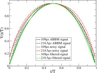
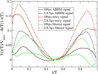
Figure S9: Simulated avalanche shapes after Wiener deconvolution for the ABBM model before and after filtering. Two durations of $109~{}\mu$s and $218~{}\mu$s shown (where each simulation time-step is taken to be $0.25~{}\mu$s as in the experiments), before and after filtering the ABBM time series with added Gaussian noise and convolved with the experimentally observed filters. (a) The differences between the ABBM and noisy shapes is significant, but after filtering the behavior is much improved. (b) After adding the noise and convolving with the impulse response function of Fig. S5(b), the average shape develops a significant asymmetry that resembles the one seen in the experiments. After filtering, this asymmetry disappears completely, since in this case we know the form of the impulse response exactly. In the case of the actual experimental shapes (cf. Fig. 2 of the main text), even though filtering reduces the present small asymmetry, it does not disappear completely, presumably because the true impulse function involves non-linear effects that are hard to identify and correct for. Also, note that the noisy signal includes a systematic correction near the edges of the shape ($t\rightarrow 0$ and $t\rightarrow T$), due to the presence of background noise.

.2 Films and dimensionality

Here we characterize our experimental film in more detail, and explain why it is not surprising that (as clearly shown in Figs 2 and 3 in the main text) they exhibit critical behavior consistent with the mean-field theory describing three-dimensional magnets.

Avalanches whose spatial extent is large compared to the thickness of the film should eventually be described by a two-dimensional theory. Indeed, for very thin films (below $200$ nm), new universality classes do appear puppin00 ; kim03 ; kimnat . For relatively thick polycrystalline ribbons (down to $45\mu$m), two of us have previously shown durin00 that Barkhausen noise shows the mean-field behavior expected for 3D interface depinning problems with strong dipolar interactions cizeau97 – the observed avalanches are small enough compared to the thickness, thus they should not be affected by the asymptotic crossover to 2D behavior. Our sample has an intermediate thickness of 1$\mu$m, and its polycrystalline state is confirmed by the x-ray structure shown in Fig. S10. The magnetization curves of Fig. S11 show the typical shape exhibited by thick films with a weak out-of-plane anisotropy, due to the stress stored in the film during the deposition and to the columnar microstructure amos08S . The in-plane magnetic properties are essentially isotropic, with domains of dense stripes having widths of the order of the thickness, as confirmed by performing MFM measurements. Such behavior is known to be absent in the experiments showing 2D behavior puppin00 ; kim03 ; kimnat .

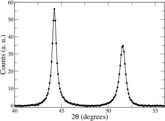
Figure S10: High angle x-ray diffraction pattern confirming the polycrystalline state of the film. The (111) and (200) permalloy peaks are identified at $2\theta\sim~{}44.2^{\circ}$, and $2\theta\sim~{}51.5^{\circ}$, respectively.

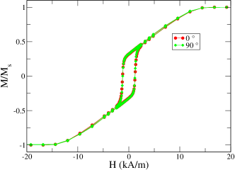
Figure S11: In-plane normalized magnetization curves measured by VSM, obtained along two different perpendicular in-plane directions $\phi=0^{\circ}$ and $\phi=90^{\circ}$. The angle $\phi$ is between the applied magnetic field and direction defined by the motion of the substrate during the deposition. The magnetization curves indicate isotropic in-plane magnetic properties with an out-of-plane anisotropy contribution, a behavior related to the stress stored in the film during the deposition, and to the columnar microstructure amos08S .

.3 Connections between the ABBM & Shell models

Here we derive in more detail the connection between the two mean-field theories (the ABBM and shell models), and then implement in detail the calculation of the paraboloic average avalanche shape for the case $k=c=0$.

The equation for the ABBM model (Eq. 2 of the main text) can be transformed to a simpler equation after taking a time derivative colaiori08S :

$$\Gamma\frac{dV}{dX}=\frac{c}{V}-k+w(X).$$ (13)

The noise term has delta-correlations in magnetization

$$\langle w(X)w(X^{\prime})\rangle_{w}=2D\delta(X-X^{\prime}).$$ (14)

Also, $dX/dt=V$ and $V\frac{d}{dX}\equiv\frac{d}{dt}$.

Eq. 13 belongs to a class of equations of the form

$$\frac{dV}{dX}=f(V)+\xi(X),$$ (15)

with

$$\langle\xi(X)\xi(X^{\prime})\rangle=\sigma_{X}^{2}\delta(X-X^{\prime}).$$ (16)

The units of $[\xi]=1/t$, so the units of $[\sigma_{X}]=\sqrt{X}/t$. We interpret Eq. 15 as a rule for incrementing $V$ and $t$ in discrete steps of size $\Delta X=\epsilon$:

$$V_{X+\epsilon}=V_{X}+\epsilon\,f(V)+\Xi(X),$$ (17)

where now $\Xi(X)$ is an uncorrelated Gaussian variable of standard deviation $\sigma_{\Xi}=\sqrt{\epsilon}\sigma_{X}$ footnote . This can be seen explicitly; $\sigma_{\Xi}$ represents the RMS width of a random walk with noise $\Xi$ of duration $\epsilon$:

$$\frac{dy}{dX} =\xi(X)$$ (18)

$$\langle(x(X+\epsilon)-x(X))^{2}\rangle =\int_{X}^{X+\epsilon}d\mu\int_{X}^{X+\epsilon}d\mu^{\prime}\langle\xi(\mu)\xi(\mu^{\prime})\rangle=\epsilon\sigma_{X}^{2},$$ (19)

using Eq. 16.

Now let us consider finding $V(t+\Delta t)$, where $\Delta t$ is large compared to $\epsilon/V$ (so many $m$-steps are averaged over) but small enough that $V$ doesn’t change significantly during the interval footnote . We do this by repeating Eq. 17, $N=V\,\Delta t/\epsilon$ times. Then

$$V(t+\Delta t) \approx V(t)+f(V)V\,\Delta t+\sum_{\tilde{X}=X(t)}^{X(t)+V\,\Delta t}\Xi(\tilde{X}).$$ (20)

The sum has $N$ terms, so is a Gaussian uncorrelated variable with standard deviation given by

$$\sqrt{N}\,\sigma_{\Xi}=\sqrt{\frac{V\Delta t}{\epsilon}}\,\sigma_{X}\sqrt{\epsilon}=\sqrt{V\Delta t}\sigma_{X}.$$ (21)

If we define a new discrete Gaussian variable $Z$ of standard deviation $\sigma_{Z}=\sqrt{\Delta t}\,\sigma_{X}$, then multiplying $Z$ by $\sqrt{V}$ mimics the sum, so we find

$$V(t+\Delta t)=V(t)+Vf(V)\,\Delta t+Z(t)\sqrt{V}.$$ (22)

If we now change to continuous time, then (analogous to Eq. 18) $\sigma_{Z}=\sigma_{\zeta}\sqrt{\Delta t}$, so

$$\frac{dV}{dt}=Vf(V)+\sqrt{V}\,\zeta(t),$$ (23)

yielding Bertotti’s result quoted in the main text. Here, $\zeta(t)$ satisfies

$$\langle\zeta(t)\zeta(t^{\prime})\rangle=\frac{\sigma_{Z}^{2}}{\Delta t}\delta(t-t^{\prime})=\sigma_{X}^{2}\delta(t-t^{\prime}).$$ (24)

From Eq. 23, the units of $[\zeta]=\sqrt{X/t^{3}}$; from Eq. 24, the units of $[\langle\zeta\zeta\rangle]=X/t^{3}$, matching the units of $[\sigma_{X}]^{2}[\delta(t)]=(X/t^{2})[1/t]$.

A nice physical idea exists behind Eq. 23: Namely, the motion $dX/dt$ is always forward, so it always uncovers “new” random forces as the front progresses. Thus the noise as a function of time must be delta-function correlated (the new sites being passed are uncorrelated with sites passed at earlier times). The key question then becomes what the strength of the delta function is: how does the noise felt by a particle moving fast over a random environment differ from that felt by a particle moving slowly? Basically, one is summing over a number of random variables proportional to $V$, so the noise is increased by a factor of square root of this number, $\sqrt{V}$.

All the above manipulations have been performed using the convenient Stratonovich interpretation. In those cases where we have calculated average shapes using the more physical Ito calculus, the results have remained unchanged, up to dimensionless constant factors. We conjecture that the two methods, although different in detail, do not differ in their predictions for universal quantities.

The temporal average avalanche shape as a first return of a random walk to the origin

Here, we show explicitly, in the simplest possible example, how one can use the concept of the first return of a random walk to the origin in order to calculate the form of the average shape’s scaling function. Let’s consider the (no-bias, constant-field) limit where $c\rightarrow 0$ and $k\rightarrow 0$, where it becomes equivalent to the so-called shell model:

$$\frac{dV}{dt}=\sqrt{V}\xi(t),$$ (25)

as described in the main text. Changing variables to $x=\sqrt{V}$, this equation becomes an ordinary random walk. We solve for an initial condition at $\epsilon$ with absorbing boundary conditions at the origin, which yields for $\epsilon\rightarrow 0$,

$$G_{RW}(x,t;\epsilon,0)=\sqrt{\frac{2}{\pi}}t^{-3/2}\epsilon~{}xe^{-x^{2}/(2t)},$$ (26)

after using the method of images. In the original $V$ coordinates it becomes:

$$G_{S}(V,t;\epsilon,0)=\frac{G_{RW}(\sqrt{V},t;\epsilon,0)}{\sqrt{V}\sqrt{\epsilon}}.$$ (27)

The average avalanche shape is defined as the average of the signal $V(t,T)$ at time $t$ for an avalanche of duration $T$. Given the probability distribution $G_{S}$, the probability of a signal $V(t,T)$ at time $t$ is $G_{S}(V,t;\epsilon,0)G_{S}(\epsilon,T;V,t)=G_{S}(V,t;\epsilon,0)G_{S}(V,t;\epsilon,T)=G_{S}(V,t;\epsilon,0)G_{S}(V,T-t;\epsilon,0)$, using time-reversal and time-translation invariance of our random walk, where $G_{S}$ has an absorbing boundary at $V=\epsilon$. In other words, the average of $V(t,T)$ naturally is

$$\langle V(t,T)\rangle = \lim_{\epsilon\rightarrow 0}\frac{\int_{0}^{\infty}dVVG_{S}(V,t;\epsilon,0)G_{S}(V,T-t;\epsilon,0)}{\int_{0}^{\infty}dVG_{S}(V,t;\epsilon,0)G_{S}(V,T-t;\epsilon,0)}$$ (28)

$$\approx 2T\left(\frac{t}{T}\left(1-\frac{t}{T}\right)\right)+O(\epsilon),$$

and therefore, the shape is an inverted parabola.

References

- (1) Wilson, K. G. The renormalization group: Critical phenomena and the Kondo problem. Rev. Mod. Phys. 47, 773–840 (1975).
- (2) Fisher, D. S. Collective transport in random media: from superconductors to earthquakes. Phys. Reports 301, 113–150 (1998).
- (3) Doussal, P. L. and Wiese, K. J. Size distributions of shocks and static avalanches from the functional renormalization group. Physical Review E 79, 051106 (2009).
- (4) Sethna, J. P., Dahmen, K., and Myers, C. R. Crackling noise. Nature 410, 242–250 (2001).
- (5) Durin, G. and Zapperi, S. volume II, chapter III ”The Barkhausen noise”, 181–267. Academic Press, Amsterdam (2006). (Preprint on cond-mat/0404512).
- (6) Mehta, A. P., Mills, A. C., Dahmen, K. A., and Sethna, J. P. Universal pulse shape scaling function and exponents: Critical test for avalanche models applied to Barkhausen noise. Phys. Rev. E 65, 046139 (2002).
- (7) Laurson, L. and Alava, M. J. 1/f noise and avalanche scaling in plastic deformation. Phys. Rev. E 74, 066106 (2006).
- (8) Chrzan D. C. and Mills M. J. Criticality in the plastic deformation of L12 intermetallic compounds, Phys. Rev. B 50, 30 –-42 (1994).
- (9) Kuntz M. C., and Sethna J. P., Noise in disordered systems: The power spectrum and dynamic exponents in avalanche models Phys. Rev. B 62, 11699–-11708 (2000).
- (10) Colaiori, F. Exactly solvable model of avalanches dynamics for Barkhausen crackling noise. Advances in Physics 57, 287–359 (2008).
- (11) Durin, G. and Zapperi, S. On the power spectrum of magnetization noise. J. Magn. Magn. Mat. 242-245, 1085 – 1088 (2002).
- (12) Zapperi, S., Castellano, C., Colaiori, F., and Durin, G. Signature of effective mass in crackling-noise asymmetry. Nature Physics 1, 46–49 (2005).
- (13) Alessandro, B., Beatrice, C., Bertotti, G., and Montorsi, A. Domain-wall dynamics and Barkhausen effect in metallic ferromagnetic materials. I. Theory. J. Appl. Phys. 68, 2901–2907 (1990).
- (14) Sethna, J. P., Dahmen, K., Kartha, S., Krumhansi, J. A., Roberts, B. W., and Shore, J. D. Hysteresis and hierarchies: Dynamics of disorder-driven first-order phase transformations. Phys. Rev. Lett. 70, 3347–3350 (1993).
- (15) Laurson, L., Illa, X., and Alava, M. J. The effect of thresholding on temporal avalanche statistics. J. Stat. Mech. , P01019 (2009).
- (16) Press, W. H., Teukolsky, S. A., Vetterling, W. T., and Flannery, B. P. Numerical Recipes in C: The art of scientific computing. Cambridge University Press, (1988).
- (17) Durin, G. and Zapperi, S., Scaling exponents for Barkhausen avalanches in polycrystalline and amorphous ferromagnets. Phys. Rev. Lett. 84, 4705–4708 (2000).
- (18) Zapperi, S., Cizeau, P., Durin, G., and Stanley, H. E. Dynamics of a ferromagnetic domain wall: Avalanches, depinning transition, and the Barkhausen effect. Phys. Rev. B 58, 6353–6366 (1998).
- (19) Zaiser, M. Scale invariance in plastic flow of crystalline solids. Adv. Phys. 55, 185–245 (2006).
- (20) Fisher, D. S., Dahmen, K., Ramanathan, S., and Ben-Zion, Y. Statistics of Earthquakes in Simple Models of Heterogeneous Faults. Phys. Rev. Lett. 78, 4885–4888 (1997).
- (21) Kwang-Su Ryu, Hiro Akinaga and Sung-Chul Shin, Tunable scaling behaviour observed in Barkhausen criticality of a ferromagnetic film Nat. Phys. 3, 547-550 (2007).
- (22) Colaiori, F., Zapperi, S., and Durin, G. Shape of a Barkhausen pulse. J. Magn. Magn. Mat. 272-276, E533–E534 (2004).
- (23) Bertotti, G. Hysteresis in Magnetism. Academic Press, San Diego, (1998).
- (24) Baldassarri, A., Colaiori, F., and Castellano, C. Average Shape of a Fluctuation: Universality in Excursions of Stochastic Processes. Phys. Rev. Lett. 90, 060601 (2003).
- (25) Kampen, N. G. V. Stochastic Processes in Physics and Chemistry. Elsevier, (2007).
- (26) Bray, A. J. Random walks in logarithmic and power-law potentials, non-universal persistence, and vortex dynamics in the two-dimensional XY model. Phys. Rev. E 62, 103 (2000).
- (27) Hubert, A. and Schäfer, R. Magnetic domains: The Analysis of Magnetic Microstructures. Springer, New York, (1998).
- (28) Viegas, A. D. C., Corrêa, M. A., Santi, L., da Silva, R. B., Bohn, F., Carara, M., and Sommer, R. L. Thickness dependence of the high-frequency magnetic permeability in amorphous Fe73.5Cu1Nb3Si13.5B9 thin films. J. Appl. Phys. 101, 033908 (2007).
- (29) Santi, L., Bohn, F., Viegas, A. D. C., Durin, G., Magni, A., Bonin, R., Zapperi, S., and Sommer, R. L. Effects of thickness on the statistical properties of the barkhausen noise in amorphous films. Physica B 384, 144–146 (2006) and Magnetostriction, Barkhausen noise and magnetization processes in E110 grade non-oriented electrical steels. J. Magn. Magn. Mater. 317, 20–28 (2007).
- (30) Bohn, F., Gündel, A., Landgraf, F. J. G., Severino, A. M., and Sommer, R. L.

References

- (1) E. Puppin, Statistical properties of Barkhausen noise in thin Fe films. Phys. Rev. Lett. 84, 5415-5418 (2000).
- (2) D.-H. Kim, S.-B. Choe, and S.-C. Shin, Direct observation of Barkhausen avalanche in Co thin films Phys. Rev. Lett. 90, 087203 (2003).
- (3) K.-S. Ryu, H. Akinaga and S-C. Shin, Tunable scaling behaviour observed in Barkhausen criticality of a ferromagnetic film Nat. Phys. 3, 547-550 (2007).
- (4) Durin, G. and Zapperi, S., Scaling exponents for Barkhausen avalanches in polycrystalline and amorphous ferromagnets. Phys. Rev. Lett. 84, 4705–4708 (2000).
- (5) Cizeau, P., Zapperi, S., Durin, G., and Stanley, H. E., Dynamics of a ferromagnetic domain wall and the Barkhausen effect. Phys. Rev. Lett. 79, 4669 (1997).
- (6) N. Amos, R. Fernandez, R. Ikkawi, B. Lee, A. Lavrenov, A. Krichevsky, D. Litvinov, and S. Khizroev, Magnetic force microscopy study of magnetic stripe domains in sputter deposited Permalloy thin films. J. Appl. Phys. 103, 07E732 (2008).
- (7) Colaiori, F. Exactly solvable model of avalanches dynamics for Barkhausen crackling noise. Adv. Phys. 57, 287–359 (2008).
- (8) Note that during the avalanche, so we don’t need to worry about not being monotone; we never re-use the random forces .