Extending the eigCG algorithm to non-symmetric linear systems with multiple right-hand sides

Abstract:

For Hermitian positive definite linear systems and eigenvalue problems, the eigCG algorithm is a memory efficient algorithm that solves the linear system and simultaneously computes some of its eigenvalues. The algorithm is based on the Conjugate-Gradient (CG) algorithm, however, it uses only a window of the vectors generated by the CG algorithm to compute approximate eigenvalues. The number and accuracy of the eigenvectors can be increased by solving more right-hand sides. For Hermitian systems with multiple right-hand sides, the computed eigenvectors can be used to speed up the solution of subsequent systems. The algorithm was tested on Lattice QCD problems by solving the normal equations and was shown to give large speed up factors and to remove the critical slowing down as we approach light quark masses. Here, an extension to the non-symmetric case based on the two-sided Lanczos algorithm is given. The new algorithm is tested on Lattice QCD problems and is shown to give very promising results. We also study the removal of the critical slowing down and compare results with those of the eigCG algorithm. We also discuss the case when the system is $\gamma_{5}$-Hermitian.

1 Introduction

Computation of various hadronic properties from Lattice QCD requires evaluation of the contribution of disconnected quark loops. This include, for example, the mass of the neutral pion, the spectrum of Isospin singlet mesons[1], and the contribution of strange sea quarks to the electromagnetic form factors of the proton[2],[3]. Evaluation of the contribution of disconnected quark loops requires knowledge of the quark propagator from all sites to all sites on the lattice (all-to-all propagators)[4, 5, 6]. In all-to-all propagator methods, one is required to compute the action of the inverse of the lattice Dirac operator $A$ on a particular set of sources $b_{i},\quad i=1,2,\dots,N_{r}$, by solving the linear systems,

$$Ax_{i}=b_{i},\quad i=1,2,\dots,N_{r}.$$ (1)

Typical values of $N_{r}$ are ${\cal{O}}(50-100)$ and large values of $N_{r}$ are required for smaller statistical noise errors. In addition, for small quark masses, solving Eqs.1 using standard iterative methods, such as GMRES or BiCGStab, converges very slowly (critical slowing down phenomena). It has been realized that critical slowing down could be removed by computing and deflating the lowest eigenmodes of $A$ (see [7] for a review of deflation methods in lattice QCD).

In [8] we have given the Incremental eigCG algorithm for Hermitian, positive definite systems. The eigCG part of the algorithm solves a single system using the Conjugate Gradient (CG) algorithm and simultaneously computes few eigenvectors with smallest eigenvalues. EigCG uses only a small size window of the CG residuals for computing eigenvalues. In addition, the standard CG part of eigCG for solving the linear system is totally unaffected by the computation of the eigenvalues. For multiple right-hand sides, Incremental eigCG solves a small subset of the linear systems using eigCG and concurrently accumulates more eigenvectors as desired. The remaining systems are then solved with CG after deflating the computed eigenvectors from the initial guesses. Incremental eigCG was tested on large Lattice QCD problems [8] with very small quark masses and was found to remove the critical slowing down as well as speed up the solution for multiple right-hand sides through deflation. Since the Dirac matrix $A$ is non-Hermitian, it was necessary to apply Incremental eigCG to the normal equations,

$$A^{\dagger}Ax_{i}=A^{\dagger}b_{i},\quad i=1,2,\dots,N_{r}.$$ (2)

In this report, we present and test an extension of the ideas of eigCG and its incremental version to the non-Hermitian case. There are three motivations for studying this extension. First, converting the non-Hermitian system 1 into the Hermitian, positive definite system 2 leads to a more difficult system as the new system will have a worse condition number. Second, solving the non-Hermitian system will give eigenvalues of $A$ directly which could be useful for other applications. Finally, one would like to compare the efficiency of removing the critical slowing down when solving the systems 1 and 2. In the extension to non-Hermitian case, we first add functionality to the BiCG algorithm, following closely what was done in the Hermitian case, that allows for computing few eigenvalues using only a limited size window of the BiCG residuals. In this case we’ll need to compute left and right eigenvectors of $A$. The modified BiCG algorithm will be called eigBiCG. For multiple right-hand sides, we solve a subset of the systems using eigBiCG and accumulate more eigenvectors and, hopefully, improve their accuracy using an incremental scheme as was done in the Hermitian case. For the remaining systems, we deflate the components of the computed eigenvectors and then use BiCGStab to solve them. Using BiCGStab instead of BiCG is motivated by the fact that BiCGStab normally converges faster than BiCG. We chose BiCG for computing eigenvectors because the BiCG residuals and parameters can easily be related to the Bi-Lanczos vectors and projection matrix. We also discuss simplifications when $A$ satisfies the $\gamma_{5}$-Hermiticity condition $\gamma_{5}A=A^{\dagger}\gamma_{5}$.

In the following, the dot product of two vectors will be denoted by $(w,v):=w^{\dagger}v$, the Euclidean norm of a vector is denoted by $||v||$ and the complex conjugate of a number $z$ will be denoted by $\bar{z}$. The function $[zr,zl,D]=eig(C)$ returns the right eigenvectors $zr$, the left eigenvectors $zl$ and the eigenvalues array $D$ sorted according to a user chosen criteria.

2 Incremental eigBiCG algorithm

In the BiLanczos algorithm one solves the dual systems $Ax=b$ and $A^{\dagger}\hat{x}=\hat{b}$. Given $x_{0}$ and $\hat{x}_{0}$ initial guesses, the algorithm builds a bi-orthogonal basis for the Krylov subspaces,

$${\cal{K}}(A,v_{1}) = \{v_{1},Av_{1},A^{2}v_{1},\dots\}$$ (3)

$$\hat{{\cal{K}}}(A^{\dagger},w_{1}) = \{w_{1},A^{\dagger}w_{1},A^{\dagger 2}w_{1},\dots\},$$

where $v_{1}=r_{0}/||r_{0}||,\ r_{0}=b-Ax_{0},$  $\hat{r}_{0}=\hat{b}-A^{\dagger}\hat{x}_{0}$ and $w_{1}=\hat{r}_{0}/(r_{0}^{\dagger}\hat{r}_{0})$, so that $w^{\dagger}_{1}v_{1}=1$. Normally, $\hat{b}=b,\ \hat{x}_{0}=x_{0},$ and $w_{1}=v_{1}$. Let $V^{(m)}=\{v_{1},v_{2},\dots,v_{m}\},\quad W^{(m)}=\{w_{1},w_{2},\dots,w_{m}\}$ be the bi-orthogonal bases of ${\cal{K}},$ and $\hat{{\cal{K}}}$, and $H^{(m)}=W^{(m)\dagger}AV^{(m)}$ the projection matrix. Let $y^{(m)}$ and $z^{(m)}$ be the right and left eigenvectors of $H^{(m)}$. The approximate right and left Ritz eigenvectors of $A$ are given by $Y^{(m)}=V^{(m)}y^{(m)}$ and $Z^{(m)}=W^{(m)}z^{(m)}$ respectively. In the BiCG algorithm, the bi-orthogonal bases $V,\ W$ and the projection matrix $H$ are not computed explicitly. The basis vectors are obtained as the right and left BiCG residuals, while the matrix $H$ is obtained from the BiCG scalar coefficients. This can be done by noting that $v_{j}=\eta_{j}r_{j-1}$ and $w_{j}=\zeta_{j}\hat{r}_{j-1}$ for $j=1,2,\dots$, with $\eta_{j}$ and $\zeta_{j}$ satisfying $(w_{j},v_{j})=1$. In the following, we choose a normalization such that $||v_{j}||=1$ and $\eta_{j}$ is real positive, however, other normalizations that maintain the biorthogonality of $w_{j}$ and $v_{j}$ could be used. From these relations, and the biorthogonality of the BiCG residuals, the elements of $H$ could be recovered from the scalar coefficients of BiCG without extra matrix-vector products.

Similar to eigCG, the eigBiCG algorithm adds functionality to the standard BiCG algorithm for computing few eigenvalues and eigenvectors of $A$ using only a window of size $m$ of the BiCG residuals. For $nev$ requested eigenvalues with a chosen criterion (smallest absolute value, for example), the eigenvalue part of eigBiCG computes eigenvectors from the size $m$ and size $(m-1)$ subspaces. The search subspaces $V^{(m)},\quad W^{(m)}$ and the projection matrix $H^{(m)}$ are then restarted with these $2nev$ computed eigenvectors which are inexpensively biorthogonalized in the coefficient space. The details of this part are given in Algorithm $BiCG-eigen$. Note that we need $m>2nev$. The full eigBiCG algorithm for solving the linear system $Ax=b$ and computing $nev$ eigenvalues and eigenvectors using a search subspace of dimension $m$ is given in Algorithm $eigBiCG$. In order to compute the elements of the $2nev+1$-th row and column of $H$ after restarting we need $Av_{2nev+1}$ and $A^{\dagger}w_{2nev+1}$ which will be given from $Ar_{j-1}$ and $A^{\dagger}\hat{r}_{j-1}$. This can be accomplished by using the relations $p_{j-1}=r_{j-1}+\beta_{j-2}p_{j-2}$ and $\hat{p}_{j-1}=\hat{r}_{j-1}+\bar{\beta}_{j-2}\hat{p}_{j-2}$. So, we need to store $Ap$ and $A^{\dagger}\hat{p}$ products when $vs=m-1$, where $vs$ is the current size of the search subspaces.

  Algorithm: $BiCG-eigen(nev,m,V^{(m)},W^{(m)},H^{(m)})$
 

• $[y^{(m)},z^{(m)},E^{(m)}]=eig(H^{(m)})$, $\quad\quad[y^{(m-1)},z^{(m-1)},E^{(m-1)}]=eig(H^{(m-1)})$.

• Append a zero at the end of each of the vectors $y^{(m-1)},z^{(m-1)}$.

• $[\tilde{y},\tilde{z}]=$ Bi-orthogonalize $[y^{(m)}_{1},y^{(m)}_{2},\dots,y^{(m)}_{nev};\quad y^{(m-1)}_{1},y^{(m-1)}_{2},\dots,y^{(m-1)}_{nev}]$ against $[z^{(m)}_{1},z^{(m)}_{2},\dots,z^{(m)}_{nev};\quad z^{(m-1)}_{1},z^{(m-1)}_{2},\dots,z^{(m-1)}_{nev}]$. Note that $y^{(m)},z^{(m)}$ are already biorthogonal. Need only to extend biorthogonality to the rest of vectors.

• $T=\tilde{z}^{\dagger}H^{(m)}\tilde{y}$, $\quad\quad[u,q,\Lambda]=eig(T)$.

• $U=V^{(m)}\tilde{y}u$, $Q=W^{(m)}\tilde{z}q$.

• Restart:

  • $V^{(m)}=[\ \ ],\quad W^{(m)}=[\ \ ]$,   $V^{(m)}_{1:2nev}=U,\quad W^{(m)}_{1:2nev}=Q$.

  • $H^{(m)}_{i,j}=0;\quad i,j=1,2,\dots,m$,   $H^{(m)}_{i,i}=\Lambda_{i}$ for $i=1,2,..,2nev$.

 

  Algorithm $Incremental\ eigBICG$
  Given initial guesses $x^{k}_{0}$ for $k=1,2,\dots,N_{r}$:

1. Choose $nev,m$ and set $U_{l}=[\quad],\quad U_{r}=[\quad]$, and $\quad H=[\quad]$.

2. For $k=1,2,\dots,n_{1}$

   • If $U_{r}$ is not empty, set $x^{k}_{0}=x^{k}_{0}+U_{r}d$, where $Hd=U_{l}^{\dagger}(b^{k}-Ax^{k}_{0})$.

   • solve the system using $eigBiCG(nev,m,V,W)$.

   • Compute $[V^{\prime},W^{\prime}]=$ biorthogonalize $[V,W]$ against $[U_{r},U_{l}]$.

   • Compute the new $H=\begin{pmatrix}H&U_{l}^{\dagger}AV^{\prime}\\ W^{\prime\dagger}AU_{r}&W^{\prime\dagger}AV^{\prime}\\ \end{pmatrix}$

   • Add the new vectors: $U_{l}=[U_{l}\quad W^{\prime}]$ and $U_{r}=[U_{r}\quad V^{\prime}]$.

3. FOR $k=n_{1}+1,n_{1}+2,\dots,N_{r}$

   • $x^{k}_{0}=x^{k}_{0}+U_{r}d$, where $Hd=U_{l}^{\dagger}(b^{k}-Ax^{k}_{0})$.

   • Solve the system using BiCGStab.

   • Repeat the deflation and restart BiCGStab when the residual is less than $DefTol*||b||$.

 

  Algorithm: $eigBiCG(nev,m,\Lambda,U,Q)$
 

1. Choose initial guess $x_{0}$, compute $r_{0}=b-Ax_{0}$, and set $p_{0}=r_{0}$.

2. Choose $\hat{r}_{0}$ such that $(\hat{r}_{0},r_{0})\neq 0$, and set $\hat{p}_{0}=\hat{r}_{0}$. Set $\rho_{0}=(\hat{r}_{0},r_{0})$, $vs=0$.

3. For $j=1,2,\dots$ till convergence

   • Compute $Ap_{j-1}$ and $A^{\dagger}\hat{p}_{j-1}$.

   • Compute $\sigma_{j-1}=(\hat{p}_{j-1},Ap_{j-1})$ and $\alpha_{j-1}=\frac{\rho_{j-1}}{\sigma_{j-1}}$. Set $x_{j}=x_{j-1}+\alpha_{j-1}p_{k-1}$.

   • If $vs=m-1$, $q=Ap_{j-1}$, $s=A^{\dagger}\hat{p}_{j-1}$.

   • If $vs=m$

     • Compute eigenvalues and restart the search subspace and projection matrix using the algorithm $BiCG-eigen(nev,m,V,W,H)$. Set $vs=2nev$.

     • Compute the $H_{k,2nev+1}$ and $H_{2nev+1,k}$ for $k=1,2,\dots,2nev$.
       $H_{2nev+1,k}=\frac{\|r_{j-1}\|}{\rho_{j-1}}(A^{\dagger}\hat{p}_{j-1}-\bar{\beta}_{j-2}s)^{\dagger}v_{k}.\quad\\ H_{k,2nev+1}=\frac{1}{\|r_{j-1}\|}w_{k}^{\dagger}(Ap_{j-1}-\beta_{j-2}q).$

   • $vs=vs+1,\quad v_{vs}=\frac{1}{\|r_{j-1}\|}r_{j-1}$, $w_{vs}=\frac{\|r_{j-1}\|}{\bar{\rho}_{j-1}}\hat{r}_{j-1}$.

   • Compute $r_{j}=r_{j-1}-\alpha_{j-1}Ap_{j-1}$ and $\hat{r}_{j}=\hat{r}_{k-1}-\bar{\alpha}_{j-1}A^{\dagger}\hat{p}_{j-1}$.

   • Set $\rho_{j}=(\hat{r}_{j},r_{j})$ and compute $\beta_{j-1}=\frac{\rho_{j}}{\rho_{j-1}}$.

   • Set $p_{j}=r_{j}+\beta_{j-1}p_{j-1}$ and $\hat{p}_{j}=\hat{r}_{j}+\bar{\beta}_{j-1}\hat{p}_{j-1}$.

   • Compute the diagonal $H$ matrix elements:
     if $j=1$, $H_{vs,vs}=\frac{1}{\alpha_{j-1}},$ else $H_{vs,vs}=\frac{1}{\alpha_{j-1}}+\frac{\beta{j-2}}{\alpha_{j-2}}$.

   • If $vs<m$, compute the off-diagonal $H$ matrix elements:
     $H_{vs,vs+1}=-\frac{\|r_{j-1}\|}{\|r_{j}\|}\frac{\beta_{j-1}}{\alpha_{j-1}},\quad H_{vs+1,vs}=-\frac{\|r_{j}\|}{\|r_{j-1}\|}\frac{1}{\alpha_{j-1}}$.

   • If $||r_{j}||\leq tol*||b||$ for a given tolerance $tol$, stop the iterations.

4. Using $V^{(vs)}$, $W^{(vs)}$ and $H^{(vs)}$ compute the final $nev$ eigenvalues and eigenvectors:
   $[y^{(vs)},z^{(vs)},\Lambda^{(vs)}]=eig(H^{(vs)}),\quad\quad U^{(nev)}=V^{(vs)}y^{(nev)},\quad\quad Q^{(nev)}=W^{(vs)}z^{(vs)}$.

 

For multiple right-hand sides, we use the Incremental eigBiCG algorithm. After solving a subset of the right-hand sides and accumulating the deflation subspaces $U_{l}$ and $U_{r}$, we use BiCGStab on the remaining systems after deflating the eigenvector components. Since computed eigenvectors are not exact we might need to repeat the deflation step and restart BiCGStab depending on the accuracy of the eigenvectors. The deflation restart tolerance is called $DefTol$. In addition, final eigenvectors computed from incremental eigBiCG could be computed, if necessary, using Raleigh-Ritz with $U_{l}$, and $U_{r}$ as search subspaces.

3 Results

The algorithm is preliminary tested on two quenched Wilson lattice QCD matrices with even-odd preconditioning near$\kappa_{critical}$. The first is a $8^{4}$ lattice at $\beta=5.5$ with $m_{q}=-1.25$ where $\kappa=\frac{1}{8+2m_{q}}$. This case will be labeled as $QCD49K-eo$ since the Dirac matrix will be of size $49,152$ before the even-odd precondtioning. The second is a $12^{4}$ lattice at $\beta=5.8$ with $m_{q}=-0.95$. This case will be labeled as $QCD249K-eo$. We first compare the lowest eigenvalues computed with eigBiCG to those computed with un-restarted BiCG in which all the residuals were stored. As seen from Table 1, the results from eigBiCG with a limited storage gives eigenvalues in close agreement with un-restarted BiCG where all the residuals were stored. We next study how incremental eigBiCG could speed up the solution with many right-hand sides. In Figure 1, we show the effect of deflation for different choices of $nev$ and $m$ after solving $n1$ right-hand sides, showing a speed up factor of about $2.5$. In Figure 2, we show the effect of reducing the quark mass on the number of iterations used by $BiCGStab$ and compare it to the case when solving the normal equations using $Incremental\ EigCG$. The results show that $Incremental\ eigBiCG$ is competitive with $eigCG$ but not necessarily better. We note that both $BiCGStab$ and $CG$ applied to the normal equations use two matrix-vector products per iteration. A better comparison between the two methods requires experiments on larger lattice QCD matrices.

Method	Eigenvalues	Residuals
eigBiCG	3.46577e-03-1.07644e-13i	1.71e-07
	1.35450e-02+1.72604e-02i	1.69e-06
	1.35450e-02-1.72604e-02i	1.37e-06
	2.82870e-02+1.09765e-07i	2.40e-03
	1.51950e-02-2.26792e-02i	9.35e-01
BiCG	3.46577e-03+7.84451e-15i	1.43e-08
	1.35450e-02+1.72604e-02i	1.72e-06
	1.35450e-02-1.72604e-02i	1.40e-06
	2.82870e-02+1.09755e-07i	2.39e-03
	1.36523e-02+4.16515e-02i	1.52e-06

Table 1: Comparing lowest 5 eigenvalues for QCD249K-eo obtained with un-restarted BiCG and with eigBiCG using $nev=15$ and $m=40$. The tolerance for the linear system was chosen to be $1e-08$ and the system converged in $592$ iterations

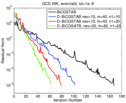
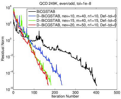
Figure 1: Deflated BiCGStab using eigenvectors computed with eigBiCG for $n1$ right-hand sides for different choices of $nev$ and $m$. No restarting was needed ($DefTol=0$ was used).

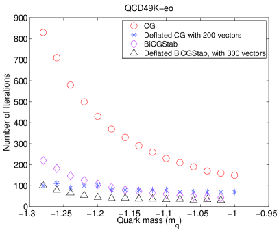
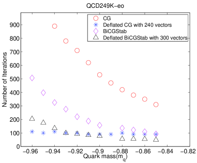
Figure 2: Removing critical slowing down using eigBiCG and eigCG applied to the normal equations.

4 $\gamma_{5}$-Hermitian systems

For Wilson and Clover fermions we have the symmetry

$$\gamma_{5}A=A^{\dagger}\gamma_{5}.$$ (4)

Using this symmetry we can replace the costly matrix-vector multiplication with $A^{\dagger}$ in eigBiCG with the cheaper multiplication with $\gamma_{5}$. In BiCG, if we chose $\hat{r}_{0}=\gamma_{5}r_{0}$ then it follows that $\hat{r}_{j}=\gamma_{5}r_{j}$ and the search directions $\hat{p}_{j}=\gamma_{5}p_{j}$ for subsequent iterations. Also, eigenvalues will be real or come in pairs of conjugate values, and left eigenvectors are computable from right ones, as long as we keep eigenvectors corresponding to conjugate pairs. Using these relations, we can simplify the first phase of $Incremental\ eigBiCG$ where eigenvalues are computed. For illustration, we show preliminary results comparing the two versions of the algorithm in Figure 3. The result shows a similar performance In which only the right eigenvectors need to be stored and where matrix-vector multiplication with $A^{\dagger}$ is avoided.

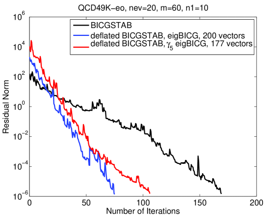
Figure 3: Comparison of deflation with $\gamma_{5}$-Hermitian algorithm.

5 Conclusions

Extending the ideas behind the successful eigCG algorithm to non-Hermitian systems gave very promising results. The new algorithm gave access to the left and right eigenvectors of the Dirac matrix while solving the linear systems using only a limited storage. It was also shown to remove the critical slowing down and to be competitive with eigCG. For $\gamma_{5}$-Hermitian systems, preliminary study shows that storage of the left eigenvectors and multiplication with $A^{\dagger}$ could be avoided.

- [1] E. B. Gregory, A. C. Irving, C. M. Richards and C. McNeile, Phys. Rev. D 77, 065019 (2008) [arXiv:0709.4224 [hep-lat]].
- [2] D. B. Leinweber et al., Phys. Rev. Lett. 97, 022001 (2006) [arXiv:hep-lat/0601025].
- [3] R. Lewis, W. Wilcox and R. M. Woloshyn, Phys. Rev. D 67, 013003 (2003) [arXiv:hep-ph/0210064].
- [4] W. Wilcox, arXiv:hep-lat/9911013.
- [5] J. Foley, K. Jimmy Juge, A. O’Cais, M. Peardon, S. M. Ryan and J. I. Skullerud, Comput. Phys. Commun. 172, 145 (2005) [arXiv:hep-lat/0505023].
- [6] M. Peardon et al. [Hadron Spectrum Collaboration], Phys. Rev. D 80 (2009) 054506 [arXiv:0905.2160 [hep-lat]].
- [7] W. Wilcox, PoS LAT2007, 025 (2007) [arXiv:0710.1813 [hep-lat]].
- [8] A. Stathopoulos and K. Orginos, arXiv:0707.0131 [hep-lat].