Discrete Hamilton–Jacobi Theory

Abstract.

We develop a discrete analogue of Hamilton–Jacobi theory in the framework of discrete Hamiltonian mechanics. The resulting discrete Hamilton–Jacobi equation is discrete only in time. We describe a discrete analogue of Jacobi’s solution and also prove a discrete version of the geometric Hamilton–Jacobi theorem. The theory applied to discrete linear Hamiltonian systems yields the discrete Riccati equation as a special case of the discrete Hamilton–Jacobi equation. We also apply the theory to discrete optimal control problems, and recover some well-known results, such as the Bellman equation (discrete-time HJB equation) of dynamic programming and its relation to the costate variable in the Pontryagin maximum principle. This relationship between the discrete Hamilton–Jacobi equation and Bellman equation is exploited to derive a generalized form of the Bellman equation that has controls at internal stages.

1. Introduction

1.1. Discrete Mechanics

Discrete mechanics is a reformulation of Lagrangian and Hamiltonian mechanics with discrete time, as opposed to a discretization of the equations in the continuous-time theory. It not only provides a systematic view of structure-preserving integrators, but also has interesting theoretical aspects analogous to continuous-time Lagrangian and Hamiltonian mechanics [see, e.g., 30; 33; 34]. The main feature of discrete mechanics is its use of discrete versions of variational principles. Namely, discrete mechanics assumes that the dynamics is defined at discrete times from the outset, formulates a discrete variational principle for such dynamics, and then derives a discrete analogue of the Euler–Lagrange or Hamilton’s equations from it.

The advantage of this construction is that it naturally gives rise to discrete analogues of the concepts and ideas in continuous time that have the same or similar properties, such as symplectic forms, the Legendre transformation, momentum maps, and Noether’s theorem [30]. This in turn provides us with the discrete ingredients that facilitate further theoretical developments, such as discrete analogues of the theories of complete integrability [see, e.g., 31; 33; 34] and also those of reduction and connections [20; 28; 25]. Whereas the main topic in discrete mechanics is the development of structure-preserving algorithms for Lagrangian and Hamiltonian systems [see, e.g., 30], the theoretical aspects of it are interesting in their own right, and furthermore provide insight into the numerical aspects as well.

Another notable feature of discrete mechanics, especially on the Hamiltonian side, is that it is a generalization of (nonsingular) discrete optimal control problems. In fact, as stated in Marsden and West [30], discrete mechanics is inspired by discrete formulations of optimal control problems (see, e.g., Jordan and Polak [21] and Cadzow [9]).

1.2. Hamilton–Jacobi Theory

In classical mechanics [see, e.g., 24; 3; 29; 16], the Hamilton–Jacobi equation is first introduced as a partial differential equation that the action integral satisfies. Specifically, let $Q$ be a configuration space and $T^{*}Q$ be its cotangent bundle; and let $q\in Q$ and $t>0$ be arbitrary and suppose that $(\hat{q}(s),\hat{p}(s))\in T^{*}Q$ is a solution of Hamilton’s equations

$$\dot{q}=\dfrac{\partial H}{\partial p},\qquad\dot{p}=-\dfrac{\partial H}{\partial q}$$ (1.1)

with the endpoint condition $\hat{q}(t)=q$. Then calculate the action integral along the solution over the time interval $[0,t]$, i.e.,

$$S(q,t)\mathrel{\mathop{:}}=\int_{0}^{t}\!\left[\hat{p}(s)\cdot\dot{\hat{q}}(s)-H(\hat{q}(s),\hat{p}(s))\right]ds,$$ (1.2)

where we regard the resulting integral as a function of the endpoint $(q,t)\in Q\times\mathbb{R}_{+}$ with $\mathbb{R}_{+}$ being the set of positive real numbers. Then by taking variation of the endpoint $(q,t)$, one obtains a partial differential equation satisfied by $S(q,t)$:

$$\dfrac{\partial S}{\partial t}+H\!\left(q,\dfrac{\partial S}{\partial q}\right)=0.$$ (1.3)

This is the Hamilton–Jacobi equation.

Conversely, it is shown that if $S(q,t)$ is a solution of the Hamilton–Jacobi equation then $S(q,t)$ is a generating function for the family of canonical transformations (or symplectic flows) that describe the dynamics defined by Hamilton’s equations. This result is the theoretical basis for the powerful technique of exact integration called separation of variables.

1.3. Connection with Optimal Control and The Hamilton–Jacobi–Bellman Equation

The idea of Hamilton–Jacobi theory is also useful in optimal control theory (see, e.g., Jurdjevic [22] and Bertsekas [6]). Consider a typical optimal control problem

$$\min_{u(\cdot)}\int_{0}^{T}C(q,u)\,dt,$$

subject to the constraints,

$$\dot{q}=f(q,u),$$

and $q(0)=q_{0}$ and $q(T)=q_{T}$. We define the augmented cost functional:

$$\hat{S}[u]\mathrel{\mathop{:}}=\int_{0}^{T}\!\left\{C(q,u)+p[\dot{q}-f(q,u)]\right\}dt=\int_{0}^{T}\!\left[p\cdot\dot{q}-\hat{H}(q,p,u)\right]dt,$$

where we introduced the costate $p$, and also defined the control Hamiltonian,

$$\hat{H}(q,p,u)\mathrel{\mathop{:}}=p\cdot f(q,u)-C(q,u).$$

Assuming that

$$\dfrac{\partial\hat{H}}{\partial u}(q,p,u)=0$$

uniquely defines the optimal control $u=u^{*}(q,p)$, we set

$$H(q,p)\mathrel{\mathop{:}}=\max_{u}\hat{H}(q,p,u)=\hat{H}\!\left(q,p,u^{*}(q,p)\right).$$

We also define the optimal cost-to-go function

$$J(q,t) \mathrel{\mathop{:}}=\int_{t}^{T}\!\left\{C(\hat{q},u^{*})+p\!\left[\dot{\hat{q}}-f(\hat{q},u^{*})\right]\right\}ds$$

$$=\int_{t}^{T}\!\left[\hat{p}\cdot\dot{\hat{q}}-H(\hat{q},\hat{p})\right]ds=S^{*}-S(q,t),$$

where $(\hat{q}(s),\hat{p}(s))$ for $s\in[0,T]$ is the solution of Hamilton’s equations with the above $H$ such that $\hat{q}(t)=q$; and $S^{*}$ is the optimal cost

$$S^{*}\mathrel{\mathop{:}}=\int_{0}^{T}\!\left[\hat{p}\cdot\dot{\hat{q}}-H(\hat{q},\hat{p})\right]ds=\int_{0}^{T}\!\left[\hat{p}\cdot\dot{\hat{q}}-\hat{H}\bigl{(}\hat{q},\hat{p},u^{*}(\hat{q},\hat{p})\bigr{)}\right]ds=\hat{S}[u^{*}],$$

and the function $S(q,t)$ is defined by

$$S(q,t)\mathrel{\mathop{:}}=\int_{0}^{t}\!\left[\hat{p}\cdot\dot{\hat{q}}-H(\hat{q},\hat{p})\right]ds.$$

Since this definition coincides with Eq. (1.2), the function $S(q,t)=S^{*}-J(q,t)$ satisfies the H–J equation (1.3); this reduces to the Hamilton–Jacobi–Bellman (HJB) equation for the optimal cost-to-go function $J(q,t)$:

$$\dfrac{\partial J}{\partial t}+\min_{u}\!\left[\dfrac{\partial J}{\partial q}\cdot f(q,u)+C(q,u)\right]=0.$$ (1.4)

It can also be shown that the costate $p$ of the optimal solution is related to the solution of the HJB equation.

1.4. Discrete Hamilton–Jacobi Theory

The main objective of this paper is to present a discrete analogue of Hamilton–Jacobi theory within the framework of discrete Hamiltonian mechanics [23], and also to apply the theory to discrete optimal control problems.

There are some previous works on discrete-time analogues of the Hamilton–Jacobi equation, such as Elnatanov and Schiff [13] and Lall and West [23]. Specifically, Elnatanov and Schiff [13] derived an equation for a generating function of a coordinate transformation that trivializes the dynamics. This derivation is a discrete analogue of the conventional derivation of the continuous-time Hamilton–Jacobi equation [see, e.g., 24, Chapter VIII]. Lall and West [23] formulated a discrete Lagrangian analogue of the Hamilton–Jacobi equation as a separable optimization problem.

1.5. Main Results

Our work was inspired by the result of Elnatanov and Schiff [13] and starts from a reinterpretation of their result in the language of discrete mechanics. This paper further extends the result by developing discrete analogues of results in (continuous-time) Hamilton–Jacobi theory. Namely, we formulate a discrete analogue of Jacobi’s solution, which relates the discrete action sum to a solution of the discrete Hamilton–Jacobi equation. This also provides a very simple derivation of the discrete Hamilton–Jacobi equation and exhibits a natural correspondence with the continuous-time theory. Another important result in this paper is a discrete analogue of the Hamilton–Jacobi theorem, which relates the solution of the discrete Hamilton–Jacobi equation with the solution of the discrete Hamilton’s equations.

We also show that the discrete Hamilton–Jacobi equation is a generalization of the discrete Riccati equation and the Bellman equation (see Fig. 1). Specifically, we show that the discrete Hamilton–Jacobi equation applied to linear discrete Hamiltonian systems and discrete optimal control problems reduces to the discrete Riccati and Bellman equations, respectively. This is again a discrete analogue of the well-known results that the Hamilton–Jacobi equation applied to linear Hamiltonian systems and optimal control problems reduces to the Riccati (see, e.g., Jurdjevic [22, p. 421]) and HJB equations (see Section 1.3 above), respectively.

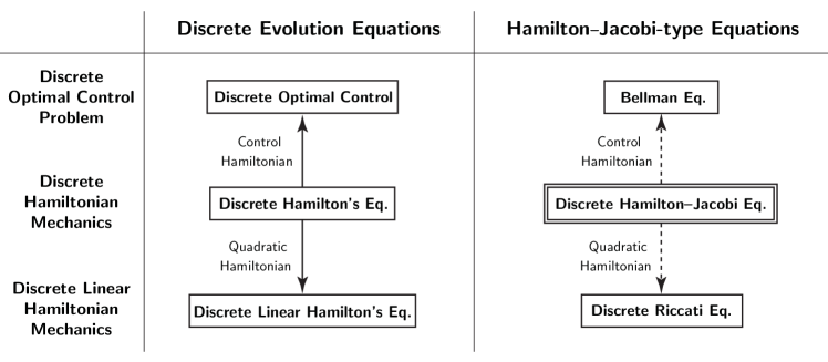
Figure 1. Discrete evolution equations (left) and corresponding discrete Hamilton–Jacobi-type equations (right). Dashed lines are the links established in the paper.

The link between the discrete Hamilton–Jacobi equation and the Bellman equation turns out to be useful in deriving a class of generalized Bellman equations that are higher-order approximations of the original continuous-time problem. Specifically, we use the idea of the Galerkin Hamiltonian variational integrator of Leok and Zhang [26] to derive discrete control Hamiltonians that yield higher-order approximations, and then show that the corresponding discrete Hamilton–Jacobi equation gives a class of Bellman equations with controls at internal stages.

1.6. Outline of the Paper

We first present a brief review of discrete Lagrangian and Hamiltonian mechanics in Section 2. In Section 3, we describe a reinterpretation of the result of Elnatanov and Schiff [13] in the language of discrete mechanics and a discrete analogue of Jacobi’s solution to the discrete Hamilton–Jacobi equation. The remainder of Section 3 is devoted to more detailed studies of the discrete Hamilton–Jacobi equation: its left and right variants, more explicit forms of them, and also a digression on the Lagrangian side. In Section 4, we prove a discrete version of the Hamilton–Jacobi theorem. In Section 5, we apply the theory to linear discrete Hamiltonian systems, and show that the discrete Riccati equation follows from the discrete Hamilton–Jacobi equation. Section 6 establishes the link with discrete-time optimal control and interprets the results of the preceding sections in this setting. Section 7 further extends this idea to derive a class of Bellman equations with controls at internal stages.

2. Discrete Mechanics

This section briefly reviews some key results of discrete mechanics following Marsden and West [30] and Lall and West [23].

2.1. Discrete Lagrangian Mechanics

A discrete Lagrangian flow $\{q_{k}\}_{k=0}^{N}$, on an $n$-dimensional differentiable manifold $Q$, can be described by the following discrete variational principle: Let $S_{\rm d}^{N}$ be the following action sum of the discrete Lagrangian $L_{\rm d}:Q\times Q\to\mathbb{R}$:

$$S_{\rm d}^{N}(\{q_{k}\}_{k=0}^{N})\mathrel{\mathop{:}}=\sum_{k=0}^{N-1}L_{\rm d}(q_{k},q_{k+1})\approx\int_{0}^{t_{N}}L(q(t),\dot{q}(t))\,dt,$$ (2.1)

which is an approximation of the action integral as shown above.

Consider discrete variations $q_{k}\mapsto q_{k}+\varepsilon\,\delta q_{k}$, for $k=0,1,\dots,N$, with $\delta q_{0}=\delta q_{N}=0$. Then, the discrete variational principle $\delta S_{\rm d}^{N}=0$ gives the discrete Euler–Lagrange equations:

$$D_{2}L_{\rm d}(q_{k-1},q_{k})+D_{1}L_{\rm d}(q_{k},q_{k+1})=0.$$ (2.2)

This determines the discrete flow $F_{L_{\rm d}}:Q\times Q\to Q\times Q$:

$$F_{L_{\rm d}}:(q_{k-1},q_{k})\mapsto(q_{k},q_{k+1}).$$ (2.3)

Let us define the discrete Lagrangian symplectic one-forms $\Theta_{L_{\rm d}}^{\pm}:Q\times Q\to T^{*}(Q\times Q)$ by

$$\Theta_{L_{\rm d}}^{+} :(q_{k},q_{k+1})\mapsto D_{2}L_{\rm d}(q_{k},q_{k+1})\,dq_{k+1},$$ (2.4a)

$$\Theta_{L_{\rm d}}^{-} :(q_{k},q_{k+1})\mapsto-D_{1}L_{\rm d}(q_{k},q_{k+1})\,dq_{k}.$$ (2.4b)

Then, the discrete flow $F_{L_{\rm d}}$ preserves the discrete Lagrangian symplectic form

$$\Omega_{L_{\rm d}}(q_{k},q_{k+1})\mathrel{\mathop{:}}=d\Theta_{L_{\rm d}}^{+}=d\Theta_{L_{\rm d}}^{-}=D_{1}D_{2}L_{\rm d}(q_{k},q_{k+1})\,dq_{k}\wedge dq_{k+1}.$$ (2.5)

Specifically, we have

$$(F_{L_{\rm d}})^{*}\Omega_{L_{\rm d}}=\Omega_{L_{\rm d}}.$$

2.2. Discrete Hamiltonian Mechanics

Introduce the right and left discrete Legendre transforms $\mathbb{F}L_{\rm d}^{\pm}:Q\times Q\to T^{*}Q$ by

$$\mathbb{F}L_{\rm d}^{+} :(q_{k},q_{k+1})\mapsto(q_{k+1},D_{2}L_{\rm d}(q_{k},q_{k+1})),$$ (2.6a)

$$\mathbb{F}L_{\rm d}^{-} :(q_{k},q_{k+1})\mapsto(q_{k},-D_{1}L_{\rm d}(q_{k},q_{k+1})),$$ (2.6b)

respectively. Then we find that the discrete Lagrangian symplectic forms Eq. (2.4) and (2.5) are pull-backs by these maps of the standard symplectic form on $T^{*}Q$:

$$\Theta_{L_{\rm d}}^{\pm}=(\mathbb{F}L_{\rm d}^{\pm})^{*}\Theta,\qquad\Omega_{L_{\rm d}}^{\pm}=(\mathbb{F}L_{\rm d}^{\pm})^{*}\Omega.$$

Let us define the momenta

$$p_{k,k+1}^{-}\mathrel{\mathop{:}}=-D_{1}L_{\rm d}(q_{k},q_{k+1}),\qquad p_{k,k+1}^{+}\mathrel{\mathop{:}}=D_{2}L_{\rm d}(q_{k},q_{k+1}).$$

Then, the discrete Euler–Lagrange equations (2.2) become simply $p_{k-1,k}^{+}=p_{k,k+1}^{-}$. So defining

$$p_{k}\mathrel{\mathop{:}}=p_{k-1,k}^{+}=p_{k,k+1}^{-},$$

one can rewrite the discrete Euler–Lagrange equations (2.2) as follows:

$$\begin{array}[]{l}\displaystyle p_{k}=-D_{1}L_{\rm d}(q_{k},q_{k+1}),\vskip 6.0pt plus 2.0pt minus 2.0pt\\ \displaystyle p_{k+1}=D_{2}L_{\rm d}(q_{k},q_{k+1}).\end{array}$$ (2.7)

Furthermore, define the discrete Hamiltonian map $\tilde{F}_{L_{\rm d}}:T^{*}Q\to T^{*}Q$ by

$$\tilde{F}_{L_{\rm d}}:(q_{k},p_{k})\mapsto(q_{k+1},p_{k+1}).$$ (2.8)

Then, one may relate this map with the discrete Legendre transforms in Eq. (2.6) as follows:

$$\tilde{F}_{L_{\rm d}}=\mathbb{F}L_{\rm d}^{+}\circ(\mathbb{F}L_{\rm d}^{-})^{-1}.$$ (2.9)

Furthermore, one can also show that this map is symplectic, i.e.,

$$(\tilde{F}_{L_{\rm d}})^{*}\Omega=\Omega.$$

This is the Hamiltonian description of the dynamics defined by the discrete Euler–Lagrange equation (2.2) introduced by Marsden and West [30]. Notice, however, that no discrete analogue of Hamilton’s equations is introduced here, although the flow is now on the cotangent bundle $T^{*}Q$.

Lall and West [23] pushed this idea further to give discrete analogues of Hamilton’s equations: From the point of view that a discrete Lagrangian is essentially a generating function of type one [16], we can apply Legendre transforms to the discrete Lagrangian to find the corresponding generating functions of type two or three [16]. In fact, they turn out to be a natural Hamiltonian counterpart to the discrete Lagrangian mechanics described above. Specifically, with the right discrete Legendre transform

$$p_{k+1}=\mathbb{F}L_{\rm d}^{+}(q_{k},q_{k+1})=D_{2}L_{\rm d}(q_{k},q_{k+1}),$$ (2.10)

we can define the following right discrete Hamiltonian:

$$H_{\rm d}^{+}(q_{k},p_{k+1})=p_{k+1}\cdot q_{k+1}-L_{\rm d}(q_{k},q_{k+1}).$$ (2.11)

Then, the discrete Hamiltonian map $\tilde{F}_{L_{\rm d}}:(q_{k},p_{k})\mapsto(q_{k+1},p_{k+1})$ is defined implicitly by the right discrete Hamilton’s equations

$$\displaystyle q_{k+1}=D_{2}H_{\rm d}^{+}(q_{k},p_{k+1}),$$ (2.12a)

$$\displaystyle p_{k}=D_{1}H_{\rm d}^{+}(q_{k},p_{k+1}),$$ (2.12b)

which are precisely the characterization of a symplectic map in terms of a generating function, $H_{\rm d}^{+}$, of type two. Similarly, with the left discrete Legendre transform

$$p_{k}=\mathbb{F}L_{\rm d}^{-}(q_{k},q_{k+1})=-D_{1}L_{\rm d}(q_{k},q_{k+1}),$$ (2.13)

we can define the following left discrete Hamiltonian:

$$H_{\rm d}^{-}(p_{k},q_{k+1})=-p_{k}\cdot q_{k}-L_{\rm d}(q_{k},q_{k+1}).$$ (2.14)

Then, we have the left discrete Hamilton’s equations

$$\displaystyle q_{k}=-D_{1}H_{\rm d}^{-}(p_{k},q_{k+1}),$$ (2.15a)

$$\displaystyle p_{k+1}=-D_{2}H_{\rm d}^{-}(p_{k},q_{k+1}),$$ (2.15b)

which corresponds to a symplectic map expressed in terms of a generation function, $H_{\rm d}^{-}$, of type three.

On the other hand, Leok and Zhang [26] demonstrate that discrete Hamiltonian mechanics can be obtained as a direct variational discretization of continuous Hamiltonian mechanics, instead of having to go via discrete Lagrangian mechanics.

3. Discrete Hamilton–Jacobi Equation

3.1. Derivation by Elnatanov and Schiff

Elnatanov and Schiff [13] derived a discrete Hamilton–Jacobi equation based on the idea that the Hamilton–Jacobi equation is an equation for a symplectic change of coordinates under which the dynamics becomes trivial. In this section, we would like to reinterpret their derivation in the framework of discrete Hamiltonian mechanics reviewed above.

Theorem 3.1.

Suppose that the discrete dynamics $\{(q_{k},p_{k})\}_{k=0}^{N}$ is governed by the right discrete Hamilton’s equations (2.12). Consider the symplectic coordinate transformation $(q_{k},p_{k})\mapsto(\hat{q}_{k},\hat{p}_{k})$ that satisfies the following:

1. The old and new coordinates are related by the type-one generating function $S^{k}:\mathbb{R}^{n}\times\mathbb{R}^{n}\to\mathbb{R}$:

   $$\begin{array}[]{l}\displaystyle\hat{p}_{k}=-D_{1}S^{k}(\hat{q}_{k},q_{k}),\vskip 6.0pt plus 2.0pt minus 2.0pt\\ \displaystyle p_{k}=D_{2}S^{k}(\hat{q}_{k},q_{k});\end{array}$$ (3.1)

2. the dynamics in the new coordinates $\{(\hat{q}_{k},\hat{p}_{k})\}_{k=0}^{N}$ is rendered trivial, i.e., $(\hat{q}_{k+1},\hat{p}_{k+1})=(\hat{q}_{k},\hat{p}_{k})$.

Then, the set of functions $\{S^{k}\}_{k=1}^{N}$ satisfies the discrete Hamilton–Jacobi equation:

$$S^{k+1}(\hat{q}_{0},q_{k+1})-S^{k}(\hat{q}_{0},q_{k})-D_{2}S^{k+1}(\hat{q}_{0},q_{k+1})\cdot q_{k+1}+H_{\rm d}^{+}\!\left(q_{k},D_{2}S^{k+1}(\hat{q}_{0},q_{k+1})\right)=0,$$ (3.2)

or, with the shorthand notation $S_{\rm d}^{k}(q_{k})\mathrel{\mathop{:}}=S^{k}(\hat{q}_{0},q_{k})$,

$$S_{\rm d}^{k+1}(q_{k+1})-S_{\rm d}^{k}(q_{k})-DS_{\rm d}^{k+1}(q_{k+1})\cdot q_{k+1}+H_{\rm d}^{+}\!\left(q_{k},DS_{\rm d}^{k+1}(q_{k+1})\right)=0.$$ (3.3)

Proof.

The key ingredient in the proof is the right discrete Hamiltonian in the new coordinates, i.e., a function $\hat{H}_{\rm d}^{+}(\hat{q}_{k},\hat{p}_{k+1})$ that satisfies

$$\begin{array}[]{l}\displaystyle\hat{q}_{k+1}=D_{2}\hat{H}_{\rm d}^{+}(\hat{q}_{k},\hat{p}_{k+1}),\vskip 6.0pt plus 2.0pt minus 2.0pt\\ \displaystyle\hat{p}_{k}=D_{1}\hat{H}_{\rm d}^{+}(\hat{q}_{k},\hat{p}_{k+1}),\end{array}$$ (3.4)

or equivalently,

$$\hat{p}_{k}\,d\hat{q}_{k}+\hat{q}_{k+1}\,d\hat{p}_{k+1}=d\hat{H}_{\rm d}^{+}(\hat{q}_{k},\hat{p}_{k+1}).$$ (3.5)

Let us first write $\hat{H}_{\rm d}^{+}$ in terms of the original right discrete Hamiltonian $H_{\rm d}^{+}$ and the generating function $S^{k}$. For that purpose, first rewrite Eqs. (2.12) and (3.1) as follows:

$$p_{k}\,dq_{k}=-q_{k+1}\,dp_{k+1}+dH_{\rm d}^{+}(q_{k},p_{k+1})$$

and

$$\hat{p}_{k}\,d\hat{q}_{k}=p_{k}\,dq_{k}-dS^{k}(\hat{q}_{k},q_{k}),$$

respectively. Then, using the above relations, we have

$$\hat{p}_{k}\,d\hat{q}_{k}+\hat{q}_{k+1}\,d\hat{p}_{k+1} =\hat{p}_{k}\,d\hat{q}_{k}+d(\hat{p}_{k+1}\cdot\hat{q}_{k+1})-\hat{p}_{k+1}\,d\hat{q}_{k+1}$$

$$=p_{k}\,dq_{k}-dS^{k}(\hat{q}_{k},q_{k})+d(\hat{p}_{k+1}\cdot\hat{q}_{k+1})-p_{k+1}\,dq_{k+1}+dS^{k+1}(\hat{q}_{k+1},q_{k+1})$$

$$=-q_{k+1}\,dp_{k+1}+dH_{\rm d}^{+}(q_{k},p_{k+1})$$

$$\quad-dS^{k}(\hat{q}_{k},q_{k})+d(\hat{p}_{k+1}\hat{q}_{k+1})-p_{k+1}\,dq_{k+1}+dS^{k+1}(\hat{q}_{k+1},q_{k+1})$$

$$=d\!\left(H_{\rm d}^{+}(q_{k},p_{k+1})+\hat{p}_{k+1}\cdot\hat{q}_{k+1}-p_{k+1}\cdot q_{k+1}+S^{k+1}(\hat{q}_{k+1},q_{k+1})-S^{k}(\hat{q}_{k},q_{k})\right).$$

Thus, in view of Eq. (3.5), we obtain

$$\hat{H}_{\rm d}^{+}(\hat{q}_{k},\hat{p}_{k+1})=H_{\rm d}^{+}(q_{k},p_{k+1})+\hat{p}_{k+1}\cdot\hat{q}_{k+1}-p_{k+1}\cdot q_{k+1}+S^{k+1}(\hat{q}_{k+1},q_{k+1})-S^{k}(\hat{q}_{k},q_{k}).$$ (3.6)

Now consider the choice of the new right discrete Hamiltonian $\hat{H}_{\rm d}^{+}$ that renders the dynamics trivial, i.e., $(\hat{q}_{k+1},\hat{p}_{k+1})=(\hat{q}_{k},\hat{p}_{k})$. It is clear from Eq. (3.4) that we can set

$$\hat{H}_{\rm d}^{+}(\hat{q}_{k},\hat{p}_{k+1})=\hat{p}_{k+1}\cdot\hat{q}_{k}.$$

Then, Eq. (3.6) becomes

$$\hat{p}_{k+1}\cdot\hat{q}_{k}=H_{\rm d}^{+}(q_{k},p_{k+1})+\hat{p}_{k+1}\cdot\hat{q}_{k+1}-p_{k+1}\cdot q_{k+1}+S^{k+1}(\hat{q}_{k+1},q_{k+1})-S^{k}(\hat{q}_{k},q_{k}),$$

and since $\hat{q}_{k+1}=\hat{q}_{k}=\dots=\hat{q}_{0}$, we have

$$0=H_{\rm d}^{+}(q_{k},p_{k+1})-p_{k+1}\cdot q_{k+1}+S^{k+1}(\hat{q}_{0},q_{k+1})-S^{k}(\hat{q}_{0},q_{k}).$$

Eliminating $p_{k+1}$ by using Eq. (3.1), we obtain Eq. (3.2). ∎

Remark 3.2.

What Elnatanov and Schiff [13] refer to as the Hamilton–Jacobi difference equation is the following:

$$S^{k+1}(\hat{q}_{0},q_{k+1})-S^{k}(\hat{q}_{0},q_{k})-D_{2}S^{k+1}(\hat{q}_{0},q_{k+1})\cdot D_{2}H_{\rm d}^{+}(q_{k},p_{k+1})+H_{\rm d}^{+}(q_{k},p_{k+1})=0.$$ (3.7)

It is clear that this is equivalent to Eq. (3.2) in view of Eq. (2.12)

3.2. Discrete Analogue of Jacobi’s Solution

This section presents a discrete analogue of Jacobi’s solution. This also gives an alternative derivation of the discrete Hamilton–Jacobi equation that is much simpler than the one shown above.

Theorem 3.3.

Consider the action sums, Eq. (2.1), written in terms of the right discrete Hamiltonian, Eq. (2.11):

$$S_{\rm d}^{k}(q_{k})\mathrel{\mathop{:}}=\sum_{l=0}^{k-1}\!\left[p_{l+1}\cdot q_{l+1}-H_{\rm d}^{+}(q_{l},p_{l+1})\right]$$ (3.8)

evaluated along a solution of the right discrete Hamilton’s equations (2.12); each $S_{\rm d}^{k}(q_{k})$ is seen as a function of the end point coordinates $q_{k}$ and the discrete end time $k$. Then, these action sums satisfy the discrete Hamilton–Jacobi equation (3.3).

Proof.

From Eq. (3.8), we have

$$S_{\rm d}^{k+1}(q_{k+1})-S_{\rm d}^{k}(q_{k})=p_{k+1}\cdot q_{k+1}-H_{\rm d}^{+}(q_{k},p_{k+1}),$$ (3.9)

where $p_{k+1}$ is considered to be a function of $q_{k}$ and $q_{k+1}$, i.e., $p_{k+1}=p_{k+1}(q_{k},q_{k+1})$. Taking the derivative of both sides with respect to $q_{k+1}$, we have

$$DS_{\rm d}^{k+1}(q_{k+1})=p_{k+1}+\dfrac{\partial p_{k+1}}{\partial q_{k+1}}\cdot\!\left[q_{k+1}-D_{2}H_{\rm d}^{+}(q_{k},p_{k+1})\right].$$

However, the terms in the brackets vanish because the right discrete Hamilton’s equations (2.12) are assumed to be satisfied. Thus, we have

$$p_{k+1}=DS_{\rm d}^{k+1}(q_{k+1}).$$ (3.10)

Substituting this into Eq. (3.9) gives Eq. (3.3). ∎

Remark 3.4.

Recall that, in the derivation of the continuous Hamilton–Jacobi equation [see, e.g., 15, Section 23], we consider the variation of the action integral, Eq. (1.2), with respect to the end point $(q,t)$ and find

$$dS=p\,dq-H(q,p)\,dt.$$ (3.11)

This gives

$$\dfrac{\partial S}{\partial t}=-H(q,p),\qquad p=\dfrac{\partial S}{\partial q},$$

and hence the Hamilton–Jacobi equation

$$\dfrac{\partial S}{\partial t}+H\!\left(q,\dfrac{\partial S}{\partial q}\right)=0.$$

In the above derivation of the discrete Hamilton–Jacobi equation (3.3), the difference in two action sums, Eq. (3.9), is a natural discrete analogue of the variation $dS$ in Eq. (3.11). Notice also that Eq. (3.9) plays the same essential role as Eq. (3.11) does in deriving the Hamilton–Jacobi equation. Table 1 summarizes the correspondence between the ingredients in the continuous and discrete theories (see also Remark 3.4).

Table 1. Correspondence between ingredients in continuous and discrete theories; $\mathbb{R}_{\geq 0}$ is the set of non-negative real numbers and $\mathbb{N}_{0}$ is the set of non-negative integers.

Continuous	Discrete
$\bigstrut(q,t)\in Q\times\mathbb{R}_{\geq 0}$	$(q_{k},k)\in Q\times\mathbb{N}_{0}$
$\displaystyle\dot{q}=\partial H/\partial p,$	$\displaystyle q_{k+1}=D_{2}H_{\rm d}^{+}(q_{k},p_{k+1})$,
$\displaystyle\dot{p}=-\partial H/\partial q$	$\displaystyle p_{k}=D_{1}H_{\rm d}^{+}(q_{k},p_{k+1})$
$\displaystyle S(q,t)\mathrel{\mathop{:}}=\int_{0}^{t}\!\left[p(s)\cdot\dot{q}(s)-H(q(s),p(s))\right]ds$	$\displaystyle S_{\rm d}^{k}(q_{k})\mathrel{\mathop{:}}=\sum_{l=0}^{k-1}\!\left[p_{l+1}\cdot q_{l+1}-H_{\rm d}^{+}(q_{l},p_{l+1})\right]$
$\displaystyle dS=\dfrac{\partial\mathstrut S}{\partial\mathstrut q}\,dq+\dfrac{\partial S}{\partial t}\,dt$	$\displaystyle S_{\rm d}^{k+1}(q_{k+1})-S_{\rm d}^{k}(q_{k})$
$\displaystyle\bigstrut p\,dq-H(q,p)\,dt$	$\displaystyle p_{k+1}\cdot q_{k+1}-H_{\rm d}^{+}(q_{k},p_{k+1})$
$\displaystyle\dfrac{\partial S}{\partial t}+H\!\left(q,\dfrac{\partial S}{\partial q}\right)=0$	$\displaystyle S_{\rm d}^{k+1}(q_{k+1})-S_{\rm d}^{k}(q_{k})-DS_{\rm d}^{k+1}(q_{k+1})\cdot q_{k+1}$
	$\displaystyle+H_{\rm d}^{+}\!\left(q_{k},DS_{\rm d}^{k+1}(q_{k+1})\right)=0$

3.3. The Right and Left Discrete Hamilton–Jacobi Equations

Recall that, in Eq. (3.8), we wrote the action sum, Eq. (2.1), in terms of the right discrete Hamiltonian, Eq. (2.11). We can also write it in terms of the left discrete Hamiltonian, Eq. (2.14), as follows:

$$S_{\rm d}^{k}(q_{k})=\sum_{l=0}^{k-1}\!\left[-p_{l}\cdot q_{l}-H_{\rm d}^{-}(p_{l},q_{l+1})\right].$$ (3.12)

Then, we can proceed as in the proof of Theorem 3.3: First, we have

$$S_{\rm d}^{k+1}(q_{k+1})-S_{\rm d}^{k}(q_{k})=-p_{k}\cdot q_{k}-H_{\rm d}^{-}(p_{k},q_{k+1}).$$ (3.13)

where $p_{k}$ is considered to be a function of $q_{k}$ and $q_{k+1}$, i.e., $p_{k}=p_{k}(q_{k},q_{k+1})$. Taking the derivative of both sides with respect to $q_{k}$, we have

$$-DS_{\rm d}^{k}(q_{k})=-p_{k}-\dfrac{\partial p_{k}}{\partial q_{k}}\cdot\!\left[q_{k}+D_{1}H_{\rm d}^{-}(p_{k},q_{k+1})\right].$$

However, the terms in the brackets vanish because the left discrete Hamilton’s equations (2.15) are assumed to be satisfied. Thus, we have

$$p_{k}=DS_{\rm d}^{k}(q_{k}).$$ (3.14)

Substituting this into Eq. (3.13) gives the discrete Hamilton–Jacobi equation with the left discrete Hamiltonian:

$$S_{\rm d}^{k+1}(q_{k+1})-S_{\rm d}^{k}(q_{k})+DS_{\rm d}^{k}(q_{k})\cdot q_{k}+H_{\rm d}^{-}\!\left(DS_{\rm d}^{k}(q_{k}),q_{k+1}\right)=0.$$ (3.15)

We refer to Eqs. (3.3) and (3.15) as the right and left discrete Hamilton–Jacobi equations, respectively.

As mentioned above, Eqs. (3.8) and (3.12) are the same action sum, Eq. (2.1), expressed in different ways. Therefore we may summarize the above argument as follows:

Proposition 3.5.

The action sums, Eq. (3.8) or equivalently Eq. (3.12), satisfy both the right and left discrete Hamilton–Jacobi equations, (3.3) and (3.15), respectively.

3.4. Explicit Forms of the Discrete Hamilton–Jacobi Equations

The expressions for the right and left discrete Hamilton–Jacobi equations in Eqs. (3.3) and (3.15) are implicit in the sense that they contain two spatial variables $q_{k}$ and $q_{k+1}$; Theorem 3.3 suggests that one may consider $q_{k}$ and $q_{k+1}$ to be related by the discrete Hamiltonian dynamics defined by either the right or left discrete Hamilton’s equations  (2.12) or (2.15), or equivalently, the discrete Hamiltonian map $\tilde{F}_{L_{\rm d}}:(q_{k},p_{k})\mapsto(q_{k+1},p_{k+1})$ defined in Eq. (2.8). More specifically, we may write $q_{k+1}$ in terms of $q_{k}$. This results in explicit forms of the discrete Hamilton–Jacobi equations, and we shall define the discrete Hamilton–Jacobi equations by the resulting explicit forms. We will see later in Section 6 that the explicit form is compatible with the formulation of the Bellman equation.

For the right discrete Hamilton–Jacobi equation (3.3), we first define the map $f^{+}_{k}:Q\to Q$ as follows: Replace $p_{k+1}$ in Eq. (2.12a) by $DS_{\rm d}^{k+1}(q_{k+1})$ as suggested by Eq. (3.10):

$$q_{k+1}=D_{2}H_{\rm d}^{+}\!\left(q_{k},DS_{\rm d}^{k+1}(q_{k+1})\right).$$

Assuming this equation is solvable for $q_{k+1}$, we define $f_{k}^{+}:Q\to Q$ by $f_{k}(q_{k})=q_{k+1}$, i.e., $f^{+}_{k}$ is implicitly defined by

$$f^{+}_{k}(q_{k})=D_{2}H_{\rm d}^{+}\!\left(q_{k},DS_{\rm d}^{k+1}(f^{+}_{k}(q_{k}))\right).$$ (3.16)

We may now identify $q_{k+1}$ with $f^{+}_{k}(q_{k})$ in the implicit form of the right Hamilton–Jacobi equation (3.3):

$$S_{\rm d}^{k+1}(f^{+}_{k}(q))-S_{\rm d}^{k}(q)-DS_{\rm d}^{k+1}(f^{+}_{k}(q))\cdot f^{+}_{k}(q)+H_{\rm d}^{+}\!\left(q,DS_{\rm d}^{k+1}(f^{+}_{k}(q))\right)=0,$$ (3.17)

where we suppressed the subscript $k$ of $q_{k}$ since it is now clear that $q_{k}$ is an independent variable as opposed to a function of the discrete time $k$. We define Eq. (3.17) to be the right discrete Hamilton–Jacobi equation. Notice that these are differential-difference-functional equations defined on $Q\times\mathbb{N}$, with the spatial variable $q$ and the discrete time $k$.

For the left discrete Hamilton–Jacobi equation (3.15), we define the map $f^{-}_{k}:Q\to Q$ as follows:

$$f^{-}_{k}(q_{k})\mathrel{\mathop{:}}=\pi_{Q}\circ\tilde{F}_{L_{\rm d}}\!\left(dS_{\rm d}^{k}(q_{k})\right),$$ (3.18)

where $\pi_{Q}:T^{*}Q\to Q$ is the cotangent bundle projection; equivalently, $f^{-}_{k}$ is defined so that the diagram below commutes.

      

Notice also that, since the map $\tilde{F}_{L_{\rm d}}:(q_{k},p_{k})\mapsto(q_{k+1},p_{k+1})$ is defined by Eq. (2.15), $f^{-}_{k}$ is defined implicitly by

$$q_{k}=-D_{1}H_{\rm d}^{-}\!\left(DS_{\rm d}^{k}(q_{k}),f^{-}_{k}(q_{k})\right).$$ (3.19)

In other words, replace $p_{k}$ in Eq. (2.15a) by $DS_{\rm d}^{k}(q_{k})$ as suggested by Eq. (3.14), and define $f_{k}^{-}(q_{k})$ as the $q_{k+1}$ in the resulting equation.

We may now identify $q_{k+1}$ with $f^{-}_{k}(q_{k})$ in Eq. (3.15):

$$S_{\rm d}^{k+1}(f^{-}_{k}(q))-S_{\rm d}^{k}(q)+DS_{\rm d}^{k}(q)\cdot q+H_{\rm d}^{-}\!\left(DS_{\rm d}^{k}(q),f^{-}_{k}(q)\right)=0,$$ (3.20)

where we again suppressed the subscript $k$ of $q_{k}$. We define Eqs. (3.17) and (3.20) to be the right and left discrete Hamilton–Jacobi equations, respectively.

Remark 3.6.

Notice that the right discrete Hamilton–Jacobi equation (3.17) is more complicated than the left one (3.20), particularly because the map $f^{+}_{k}$ appears more often than $f^{-}_{k}$ does in the latter; notice here that, as shown in Eq. (3.18), the maps $f^{\pm}_{k}$ in the discrete Hamilton–Jacobi equations (3.17) and (3.20) depend on the function $S_{\rm d}^{k}$, which is the unknown one has to solve for.

However, it is possible to define an equally simple variant of the right discrete Hamilton–Jacobi equation by writing $q_{k-1}$ in terms of $q_{k}$: Let us first define $g_{k}:Q\to Q$ by

$$g_{k}(q_{k})\mathrel{\mathop{:}}=\pi_{Q}\circ\tilde{F}_{L_{\rm d}}^{-1}\!\left(dS_{\rm d}^{k}(q_{k})\right),$$

or so that the diagram below commutes.

      

Now, in Eq. (3.3), change the indices from $(k,k+1)$ to $(k-1,k)$ and identify $q_{k-1}$ with $g_{k}(q_{k})$ to obtain

$$S_{\rm d}^{k}(q)-S_{\rm d}^{k-1}(g_{k}(q))-DS_{\rm d}^{k}(q)\cdot q+H_{\rm d}^{+}\!\left(g_{k}(q),DS_{\rm d}^{k}(q)\right)=0,$$

where we again suppressed the subscript $k$ of $q_{k}$. This is as simple as the left discrete Hamilton–Jacobi equation (3.20). However the map $g_{k}$ is, being backward in time, rather unnatural compared to $f_{k}$. Furthermore, as we shall see in Section 6, in the discrete optimal control setting, the map $f_{k}$ is defined by a given function and thus the formulation with $f_{k}$ will turn out to be more convenient.

3.5. The Discrete Hamilton–Jacobi Equation on the Lagrangian Side

First, notice that Eq. (2.1) gives

$$S_{\rm d}^{k+1}(q_{k+1})-S_{\rm d}^{k}(q_{k})=L_{\rm d}(q_{k},q_{k+1}).$$ (3.21)

This is essentially the Lagrangian equivalent of the discrete Hamilton–Jacobi equation (3.17) as Lall and West [23] suggest. Let us apply the same argument as above to obtain the explicit form for Eq. (3.21). Taking the derivative of the above equation with respect to $q_{k}$, we have

$$-D_{1}L_{\rm d}(q_{k},q_{k+1})\,dq_{k}=dS_{\rm d}^{k}(q_{k}),$$

and hence from the definition of the left discrete Legendre transform, Eq. (2.6b),

$$\mathbb{F}L_{\rm d}^{-}(q_{k},q_{k+1})=dS_{\rm d}^{k}(q_{k}).$$

Assuming that $\mathbb{F}L_{\rm d}^{-}$ is invertible, we have

$$(q_{k},q_{k+1})=(\mathbb{F}L_{\rm d}^{-})^{-1}\!\left(dS_{\rm d}^{k}(q_{k})\right)=\mathrel{\mathop{:}}(q_{k},f^{L}_{k}(q_{k})),$$

where we defined the map $f^{L}_{k}:Q\to Q$ as follows (see the commutative diagram below):

$$f^{L}_{k}(q_{k})\mathrel{\mathop{:}}=pr_{2}\circ(\mathbb{F}L_{\rm d}^{-})^{-1}\!\left(dS_{\rm d}^{k}(q_{k})\right),$$ (3.22)

where $pr_{2}:Q\times Q\to Q$ is the projection to the second factor, i.e., $pr_{2}(q_{1},q_{2})=q_{2}$. Thus, eliminating $q_{k+1}$ from Eq. (3.21) and then replacing $q_{k}$ by $q$, we obtain the discrete Hamilton–Jacobi equation on the Lagrangian side:

$$S_{\rm d}^{k+1}(f^{L}_{k}(q))-S_{\rm d}^{k}(q)=L_{\rm d}\!\left(q,f^{L}_{k}(q)\right).$$ (3.23)

The map $f^{L}_{k}$ defined in Eq. (3.22) is identical to $f^{-}_{k}$ defined above in Eq. (3.18) as the commutative diagram below demonstrates.

      

The commutativity of the square in the diagram defines the $f^{-}_{k}$ as we saw earlier, whereas that of the right-angled triangle on the lower left defines the $f^{L}_{k}$ in Eq. (3.22); note the relation $\tilde{F}_{L_{\rm d}}=\mathbb{F}L_{\rm d}^{+}\circ(\mathbb{F}L_{\rm d}^{-})^{-1}$ from Eq. (2.9).

The map $f^{L}_{k}$ being identical to $f^{-}_{k}$ implies that the discrete Hamilton–Jacobi equations on the Hamiltonian and Lagrangian sides, Eqs. (3.20) and (3.23), are equivalent.

4. Discrete Hamilton–Jacobi Theorem

The following gives a discrete analogue of the geometric Hamilton–Jacobi theorem by Abraham and Marsden [1, Theorem 5.2.4]:

Theorem 4.1 (Discrete Hamilton–Jacobi).

Suppose that $S_{\rm d}^{k}$ satisfies the right discrete Hamilton–Jacobi equation (3.17), and let $\{c_{k}\}_{k=0}^{N}\subset Q$ be a set of points such that

$$c_{k+1}=f^{+}_{k}(c_{k})\quad\text{for}\quad k=0,1,\dots,N-1.$$ (4.1)

Then, the set of points $\{(c_{k},p_{k})\}_{k=0}^{N}\subset T^{*}Q$ with

$$p_{k}\mathrel{\mathop{:}}=DS_{\rm d}^{k}(c_{k})$$ (4.2)

is a solution of the right discrete Hamilton’s equations (2.12).

Similarly, suppose that $S_{\rm d}^{k}$ satisfies the left discrete Hamilton–Jacobi equation (3.20), and let $\{c_{k}\}_{k=0}^{N}\subset Q$ be a set of points that satisfy

$$c_{k+1}=f^{-}_{k}(c_{k})\quad\text{for}\quad k=0,1,\dots,N-1.$$ (4.3)

Furthermore, assume that the Jacobian $Df^{-}_{k}$ is invertible at each point $c_{k}$. Then, the set of points $\{(c_{k},p_{k})\}_{k=0}^{N}\subset T^{*}Q$ with

$$p_{k}\mathrel{\mathop{:}}=DS_{\rm d}^{k}(c_{k})$$ (4.4)

is a solution of the left discrete Hamilton’s equations (2.15).

Proof.

To prove the first assertion, first recall the implicit definition of $f^{+}_{k}$ in Eq. (3.16):

$$f^{+}_{k}(q)=D_{2}H_{\rm d}^{+}\!\left(q,DS_{\rm d}^{k+1}(f^{+}_{k}(q))\right).$$ (4.5)

In particular, for $q=c_{k}$, we have

$$c_{k+1}=D_{2}H_{\rm d}^{+}\!\left(c_{k},p_{k}\right),$$ (4.6)

where we used Eq. (4.1) and (4.2). On the other hand, taking the derivative of Eq. (3.17) with respect to $q$,

$$DS_{\rm d}^{k+1}(f^{+}_{k}(q))\cdot Df^{+}_{k}(q)-DS_{\rm d}^{k}(q)-Df^{+}_{k}(q)\cdot D^{2}S_{\rm d}^{k+1}(f^{+}_{k}(q))\cdot f^{+}_{k}(q)-DS_{\rm d}^{k+1}(f^{+}_{k}(q))\cdot Df^{+}_{k}(q)\\ +D_{1}H_{\rm d}^{+}\!\left(q,DS_{\rm d}^{k+1}(f^{+}_{k}(q))\right)+D_{2}H_{\rm d}^{+}\!\left(q,DS_{\rm d}^{k+1}(f^{+}_{k}(q))\right)\cdot D^{2}S_{\rm d}^{k+1}(f^{+}_{k}(q))\cdot Df^{+}_{k}(q)=0,$$

which reduces to

$$-DS_{\rm d}^{k}(q)+D_{1}H_{\rm d}^{+}\!\left(q,DS_{\rm d}^{k+1}(f^{+}_{k}(q))\right)=0,$$

due to Eq. (4.5). Then, substituting $q=c_{k}$ gives

$$-DS_{\rm d}^{k}(c_{k})+D_{1}H_{\rm d}^{+}\!\left(c_{k},DS_{\rm d}^{k+1}(f^{+}_{k}(c_{k}))\right)=0.$$

Using Eqs. (4.1) and (4.2), we obtain

$$p_{k}=D_{1}H_{\rm d}^{+}\!\left(c_{k},p_{k+1}\right).$$ (4.7)

Eqs. (4.6) and (4.7) show that the sequence $\{(c_{k},p_{k})\}$ satisfies the right discrete Hamilton’s equations (2.12).

Now, let us prove the latter assertion. First, recall the implicit definition of $f^{-}_{k}$ in Eq. (3.19):

$$q=-D_{1}H_{\rm d}^{-}\!\left(DS_{\rm d}^{k}(q),f^{-}_{k}(q)\right)$$ (4.8)

In particular, for $q=c_{k}$, we have

$$c_{k}=-D_{1}H_{\rm d}^{-}\!\left(p_{k},c_{k+1}\right),$$ (4.9)

where we used Eq. (4.3) and (4.4). On the other hand, taking the derivative of Eq. (3.17) with respect to $q$ yields,

$$DS_{\rm d}^{k+1}(f^{-}_{k}(q))\cdot Df^{-}_{k}(q)-DS_{\rm d}^{k}(q)+D^{2}S_{\rm d}^{k}(q)\cdot q+DS_{\rm d}^{k}(q)\\ +D_{1}H_{\rm d}^{-}\!\left(DS_{\rm d}^{k}(q),f^{-}_{k}(q)\right)\cdot D^{2}S_{\rm d}^{k}(q)+D_{2}H_{\rm d}^{-}\!\left(DS_{\rm d}^{k}(q),f^{-}_{k}(q)\right)\cdot Df^{-}_{k}(q)=0,$$

which reduces to

$$\!\left[DS_{\rm d}^{k+1}(f^{-}_{k}(q))+D_{2}H_{\rm d}^{-}\!\left(DS_{\rm d}^{k}(q),f^{-}_{k}(q)\right)\right]\cdot Df^{-}_{k}(q)=0,$$

due to Eq. (4.8). Then, substituting $q=c_{k}$ gives

$$DS_{\rm d}^{k+1}(f^{-}_{k}(c_{k}))=-D_{2}H_{\rm d}^{-}\!\left(DS_{\rm d}^{k}(c_{k}),f^{-}_{k}(c_{k})\right),$$

since $Df^{-}_{k}(c_{k})$ is invertible by assumption. Then, using Eqs. (4.3) and (4.4), we obtain

$$p_{k+1}=-D_{2}H_{\rm d}^{-}\!\left(p_{k},c_{k+1}\right).$$ (4.10)

Eqs. (4.9) and (4.10) show that the sequence $\{(c_{k},p_{k})\}$ satisfies the left discrete Hamilton’s equations (2.15). ∎

5. Application To Discrete Linear Hamiltonian Systems

5.1. Discrete Linear Hamiltonian Systems and Matrix Riccati Equation

Example 5.1 (Quadratic discrete Hamiltonian—discrete linear Hamiltonian systems).

Consider a discrete Hamiltonian system on $T^{*}\mathbb{R}^{n}\cong\mathbb{R}^{n}\times\mathbb{R}^{n}$ (the configuration space is $Q=\mathbb{R}^{n}$) defined by the quadratic left discrete Hamiltonian

$$H_{\rm d}^{-}(p_{k},q_{k+1})=\frac{1}{2}p_{k}^{T}M^{-1}p_{k}+p_{k}^{T}Lq_{k+1}+\frac{1}{2}q_{k+1}^{T}Kq_{k+1},$$ (5.1)

where $M$, $K$, and $L$ are real $n\times n$ matrices; we assume that $M$ and $L$ are invertible and also that $M$ and $K$ are symmetric. The left discrete Hamilton’s equations (2.15) are

$$\begin{array}[]{l}\displaystyle q_{k}=-(M^{-1}p_{k}+Lq_{k+1}),\vskip 6.0pt plus 2.0pt minus 2.0pt\\ \displaystyle p_{k+1}=-(L^{T}p_{k}+Kq_{k+1}),\end{array}$$

or

$$\begin{pmatrix}q_{k+1}\vskip 6.0pt plus 2.0pt minus 2.0pt\\ p_{k+1}\end{pmatrix}=\begin{pmatrix}-L^{-1}&-L^{-1}M^{-1}\vskip 6.0pt plus 2.0pt minus 2.0pt\\ KL^{-1}&KL^{-1}M^{-1}-L^{T}\end{pmatrix}\begin{pmatrix}q_{k}\vskip 6.0pt plus 2.0pt minus 2.0pt\\ p_{k}\end{pmatrix}.$$ (5.2)

and hence are a discrete linear Hamiltonian system (see Section A.1).

Now, let us solve the left discrete Hamilton–Jacobi equation (3.20) for this system. For that purpose, we first generalize the problem to that with a set of initial points instead of a single initial point $(q_{0},p_{0})$. More specifically, consider the set of initial points that is a Lagrangian affine space $\tilde{\mathcal{L}}_{z_{0}}$ (see Definition A.2) which contains the point $z_{0}\mathrel{\mathop{:}}=(q_{0},p_{0})$. Then, the dynamics is formally written as, for any discrete time $k\in\mathbb{N}$,

$$\tilde{\mathcal{L}}^{(k)}\mathrel{\mathop{:}}=(\tilde{F}_{L_{\rm d}})^{k}\!\left(\tilde{\mathcal{L}}_{z_{0}}\right)=\underbrace{\tilde{F}_{L_{\rm d}}\circ\dots\circ\tilde{F}_{L_{\rm d}}}_{k}\!\left(\tilde{\mathcal{L}}_{z_{0}}\right),$$

where $\tilde{F}_{L_{\rm d}}:T^{*}Q\to T^{*}Q$ is the discrete Hamiltonian map defined in Eq. (2.8). Since $\tilde{F}_{L_{\rm d}}$ is a symplectic map, Proposition A.4 implies that $\tilde{\mathcal{L}}^{(k)}$ is a Lagrangian affine space. Then, assuming that $\tilde{\mathcal{L}}^{(k)}$ is transversal to $\{0\}\oplus Q^{*}$, Corollary A.6 implies that there exists a set of functions $S_{\rm d}^{k}$ of the form

$$S_{\rm d}^{k}(q)=\frac{1}{2}q^{T}A_{k}q+b_{k}^{T}q+c_{k},$$ (5.3)

such that $\tilde{\mathcal{L}}^{(k)}=\mathop{\mathrm{graph}}\nolimits dS_{\rm d}^{k}$; here $A_{k}$ are symmetric $n\times n$ matrices, $b_{k}$ are elements in $\mathbb{R}^{n}$, and $c_{k}$ are in $\mathbb{R}$.

Now that we know the form of the solution, we substitute the above expression into the discrete Hamilton–Jacobi equation to find the equations for $A_{k}$, $b_{k}$, and $c_{k}$. Notice first that the map $f^{-}_{k}$ is given by the first half of Eq. (5.2) with $p_{k}$ replaced by $DS_{\rm d}^{k}(q)$:

$$f^{-}_{k}(q) =-L^{-1}\!\left(q+M^{-1}DS_{\rm d}^{k}(q)\right)$$

$$=-L^{-1}(I+M^{-1}A_{k})q-L^{-1}M^{-1}b_{k}.$$ (5.4)

Then, substituting Eq. (5.3) into the left-hand side of the left discrete Hamilton–Jacobi equation (3.20) yields the following recurrence relations for $A_{k}$, $b_{k}$, and $c_{k}$:

$$A_{k+1} =L^{T}(I+A_{k}M^{-1})^{-1}A_{k}L-K,$$ (5.5a)

$$b_{k+1} =-L^{T}(I+A_{k}M^{-1})^{-1}b_{k},$$ (5.5b)

$$c_{k+1} =c_{k}-\frac{1}{2}b_{k}^{T}(M+A_{k})^{-1}b_{k},$$ (5.5c)

where we assumed that $I+A_{k}M^{-1}$ is invertible.

Remark 5.2.

For the $A_{k+1}$ defined by Eq. (5.5a) to be symmetric, it is sufficient that $A_{k}$ is invertible; for if it is, then Eq. (5.5a) becomes

$$A_{k+1}=L^{T}(A_{k}^{-1}+M^{-1})^{-1}L-K,$$

and so $A_{k}$, $M$, and $K$ being symmetric implies that $A_{k+1}$ is as well.

Remark 5.3.

We can rewrite Eq. (5.5a) as follows:

$$A_{k+1}=\!\left[KL^{-1}+(KL^{-1}M^{-1}-L^{T})A_{k}\right](-L^{-1}-L^{-1}M^{-1}A_{k})^{-1}.$$ (5.6)

Notice the exact correspondence between the coefficients in the above equation and the matrix entries in the discrete linear Hamiltonian equations (5.2). In fact, this is the discrete Riccati equation that corresponds to the iteration defined by Eq. (5.2). See Ammar and Martin [2] for details on this correspondence.

To summarize the above observation, we have:

Proposition 5.4.

The discrete Hamilton–Jacobi equation (3.20) applied to the discrete linear Hamiltonian system (5.2) yields the discrete Riccati equation (5.6).

In other words, the discrete Hamilton–Jacobi equation is a nonlinear generalization of the discrete Riccati equation.

6. Relation to the Bellman Equation

In this section, we apply the above results to the optimal control setting. We will show that the (right) discrete Hamilton–Jacobi equation (3.17) gives the Bellman equation (discrete-time HJB equation) as a special case. This result gives a discrete analogue of the relationship between the H–J and HJB equations discussed in Section 1.3.

6.1. Discrete Optimal Control Problem

Let $q_{\rm d}\mathrel{\mathop{:}}=\{q_{k}\}_{k=0}^{N}$ be the state variables in a vector space $V\cong\mathbb{R}^{n}$ with $q_{0}$ and $q_{N}$ fixed and $u_{\rm d}\mathrel{\mathop{:}}=\{u_{k}\}_{k=0}^{N-1}$ be controls in the set $\mathcal{U}\subset\mathbb{R}^{m}$. With a given function $C_{\rm d}:V\times\mathcal{U}\to\mathbb{R}$, define the discrete cost functional

$$J_{\rm d}\mathrel{\mathop{:}}=\sum_{k=0}^{N-1}C_{\rm d}(q_{k},u_{k}).$$

Then, we formulate the Standard Discrete Optimal Control Problem as follows [see, e.g., 21; 9; 4; 17]:

Problem 6.1 (Standard Discrete Optimal Control Problem).

Minimize the discrete cost functional, i.e.,

$$\min_{u_{\rm d}}J_{\rm d}=\min_{u_{\rm d}}\sum_{k=0}^{N-1}C_{\rm d}(q_{k},u_{k}),$$ (6.1)

subject to the constraint,

$$q_{k+1}=f_{\rm d}(q_{k},u_{k}).$$ (6.2)

6.2. Necessary Condition for Optimality and the Bellman Equation

We would like to formulate the necessary condition for optimality. First, introduce the augmented discrete cost functional:

$$\hat{S}_{\rm d}(q_{\rm d},p_{\rm d},u_{\rm d}) \mathrel{\mathop{:}}=\sum_{k=0}^{N-1}\!\left\{C_{\rm d}(q_{k},u_{k})+p_{k+1}\cdot\!\left[q_{k+1}-f_{\rm d}(q_{k},u_{k})\right]\right\}$$

$$=\sum_{k=0}^{N-1}\!\left[p_{k+1}\cdot q_{k+1}-\hat{H}_{\rm d}^{+}(q_{k},p_{k+1},u_{k})\right],$$

where we introduced the costate $p_{\rm d}\mathrel{\mathop{:}}=\{p_{k}\}_{k=1}^{N}$ with $p_{k}\in V^{*}$, and also defined the discrete control Hamiltonian

$$\hat{H}_{\rm d}^{+}(q_{k},p_{k+1},u_{k})\mathrel{\mathop{:}}=p_{k+1}\cdot f_{\rm d}(q_{k},u_{k})-C_{\rm d}(q_{k},u_{k}).$$ (6.3)

Then, the optimality condition, Eq. (6.1), is restated as

$$\min_{q_{\rm d},p_{\rm d},u_{\rm d}}\hat{S}_{\rm d}(q_{\rm d},p_{\rm d},u_{\rm d})=\min_{q_{\rm d},p_{\rm d},u_{\rm d}}\sum_{k=0}^{N-1}\!\left[p_{k+1}\cdot q_{k+1}-\hat{H}_{\rm d}^{+}(q_{k},p_{k+1},u_{k})\right].$$

In particular, extremality with respect to the control $u_{\rm d}$ implies

$$D_{3}\hat{H}_{\rm d}^{+}(q_{k},p_{k+1},u_{k})=0,\quad k=0,1,\dots,N-1.$$ (6.4)

Now, we assume that $\hat{H}_{\rm d}^{+}$ is sufficiently regular so that this equation uniquely determines the optimal control $u_{\rm d}^{*}\mathrel{\mathop{:}}=\{u_{k}^{*}\}_{k=0}^{N-1}$; and therefore, $u_{k}^{*}$ is a function of $q_{k}$ and $p_{k+1}$, i.e., $u_{k}^{*}=u_{k}^{*}(q_{k},p_{k+1})$. We then define

$$H_{\rm d}^{+}(q_{k},p_{k+1}) \mathrel{\mathop{:}}=\max_{u_{k}}\hat{H}_{\rm d}^{+}(q_{k},p_{k+1},u_{k})$$

$$=\max_{u_{k}}\!\left[p_{k+1}\cdot f_{\rm d}(q_{k},u_{k})-C_{\rm d}(q_{k},u_{k})\right]$$

$$=p_{k+1}\cdot f_{\rm d}(q_{k},u_{k}^{*})-C_{\rm d}(q_{k},u_{k}^{*}),$$ (6.5)

and also the optimal discrete cost-to-go function

$$J_{\rm d}^{k}(q_{k}) \mathrel{\mathop{:}}=\sum_{l=k}^{N-1}\!\left\{C_{\rm d}(q_{l},u_{l}^{*})+p_{l+1}\cdot\!\left[q_{l+1}-f_{\rm d}(q_{l},u_{l}^{*})\right]\right\}$$

$$=\sum_{l=k}^{N-1}\!\left[p_{l+1}\cdot q_{l+1}-H_{\rm d}^{+}(q_{l},p_{l+1})\right]$$

$$=S_{\rm d}^{*}-S_{\rm d}^{k}(q_{k}),$$ (6.6)

where $S_{\rm d}^{*}$ is the optimal discrete cost functional, i.e.,

$$S_{\rm d}^{*}\mathrel{\mathop{:}}=\hat{S}_{\rm d}(q_{\rm d},p_{\rm d},u_{\rm d}^{*})=\sum_{k=0}^{N-1}\!\left[p_{k+1}\cdot q_{k+1}-H_{\rm d}^{+}(q_{k},p_{k+1})\right].$$

and

$$S_{\rm d}^{k}(q_{k})\mathrel{\mathop{:}}=\sum_{l=0}^{k-1}\!\left[p_{l+1}\cdot q_{l+1}-H_{\rm d}^{+}(q_{l},p_{l+1})\right].$$

The above action sum has exactly the same form as Eq. (3.8) formulated in the framework of discrete Hamiltonian mechanics. Therefore, our theory now directly applies to this case: The corresponding right discrete Hamilton’s equations (2.12) are, using the expression in Eq. (6.5),

$$\begin{array}[]{l}\displaystyle q_{k+1}=f_{\rm d}(q_{k},u_{k}^{*}),\vskip 6.0pt plus 2.0pt minus 2.0pt\\ \displaystyle p_{k}=p_{k+1}\cdot D_{1}f_{\rm d}(q_{k},u_{k}^{*})-D_{1}C_{\rm d}(q_{k},u_{k}^{*}).\end{array}$$

Therefore, Eq. (3.16) gives the implicit definition of $f^{+}_{k}$ as follows:

$$f^{+}_{k}(q_{k})=f_{\rm d}\!\left(q_{k},u_{k}^{*}\!\left(q_{k},DS_{\rm d}^{k+1}(f^{+}_{k}(q_{k}))\right)\right).$$ (6.7)

Hence, the (right) discrete Hamilton–Jacobi equation (3.17) applied to this case gives

$$S_{\rm d}^{k+1}(f_{\rm d}(q_{k},u_{k}^{*}))-S_{\rm d}^{k}(q_{k})-DS_{\rm d}^{k+1}(f_{\rm d}(q_{k},u_{k}^{*}))\cdot f_{\rm d}(q_{k},u_{k}^{*})+H_{\rm d}^{+}\!\left(q_{k},DS_{\rm d}^{k+1}(f_{\rm d}(q_{k},u_{k}^{*}))\right)=0,$$

and again using the expression for the Hamiltonian in Eq. (6.5), this becomes

$$\max_{u_{k}}\!\left[S_{\rm d}^{k+1}(f_{\rm d}(q_{k},u_{k}))-C_{\rm d}(q_{k},u_{k})\right]=S_{\rm d}^{k}(q_{k}).$$

Since $S_{\rm d}^{k}(q_{k})=S_{\rm d}^{*}-J_{\rm d}^{k}(q_{k})$, we obtain

$$\min_{u_{k}}\!\left[J_{\rm d}^{k+1}(f_{\rm d}(q_{k},u_{k}))+C_{\rm d}(q_{k},u_{k})\right]=J_{\rm d}^{k}(q_{k}),$$ (6.8)

which is the Bellman equation (see, e.g., Bellman [4, 5] and Bertsekas [6]).

Remark 6.2.

Notice that the discrete HJB equation (6.8) is much simpler than the discrete Hamilton–Jacobi equations (3.17) and (3.20) because of the special form of the control Hamiltonian Eq. (6.5). Also, notice that, as shown in Eq. (6.7), the term $f^{+}_{k}(q_{k})$ is written in terms of the given function $f$. See Remark 3.6 for comparison.

6.3. Relation between the Discrete H–J and Bellman Equations and its Consequences

Summarizing the observation made above, we have

Proposition 6.3.

The right discrete Hamilton–Jacobi equation (3.17) applied to the Hamiltonian formulation of the Standard Discrete Optimal Control Problem 6.1 gives the Bellman equation (6.8).

This observation leads to the following well-known fact:

Proposition 6.4.

Let $J_{\rm d}^{k}(q_{k})$ be a solution to the Bellman equation (6.8). Then, the costate $p_{k}$ in the discrete maximum principle is given as follows:

$$p_{k}=-DJ_{\rm d}^{k}(c_{k}),$$

where $c_{k+1}=f_{\rm d}(c_{k},u_{k}^{*})$ with the optimal control $u_{k}^{*}$.

Proof.

Follows from a reinterpretation of Theorem 4.1 through Proposition 6.3 with the relation $S_{\rm d}^{k}(q_{k})=S_{\rm d}^{*}-J_{\rm d}^{k}(q_{k})$. ∎

7. Generalized Bellman Equation with Internal-Stage Controls

In the previous section, we showed that the discrete Hamilton–Jacobi equation recovers the Bellman equation if we apply our theory to the Hamiltonian formulation of the Standard Discrete Optimal Control Problem 6.1. In this section, we generalize the approach to derive what may be considered as higher-order discrete-time approximations of the HJB equation (1.4). Namely, we derive a class of discrete control Hamiltonians that use higher-order approximations (a more general version of Eq. (6.3)) by employing the technique of Galerkin Hamiltonian variational integrators introduced by Leok and Zhang [26]; and then, we apply our theory to obtain a class of generalized Bellman equations that have controls at internal stages.

7.1. Continuous-Time Optimal Control Problem

Let us first briefly review the standard formulation of continuous-time optimal control problems. Let $q$ be the state variable in a vector space $V\cong\mathbb{R}^{n}$, $q_{0}$ and $q_{T}$ fixed in $V$, and $u$ be the control in the set $\mathcal{U}\subset\mathbb{R}^{m}$. With a given function $C:V\times\mathcal{U}\to\mathbb{R}$, define the cost functional

$$J\mathrel{\mathop{:}}=\int_{0}^{T}C(q(t),u(t))\,dt.$$

Then, we formulate the Standard Continuous-Time Optimal Control Problem as follows:

Problem 7.1 (Standard Continuous-Time Optimal Control Problem).

Minimize the cost functional, i.e.,

$$\min_{u(\cdot)}J=\min_{u(\cdot)}\int_{0}^{T}C(q(t),u(t))\,dt,$$

subject to the constraints,

$$\dot{q}=f(q,u),$$

and $q(0)=q_{0}$ and $q(T)=q_{T}$.

A Hamiltonian structure comes into play with the introduction of the augmented cost functional:

$$\hat{S} \mathrel{\mathop{:}}=\int_{0}^{T}\!\left\{C(q(t),u(t))+p(t)\!\left[\dot{q}(t)-f(q(t),u(t))\right]\right\}dt$$

$$=\int_{0}^{T}\!\left[p(t)\dot{q}(t)-\hat{H}(q(t),p(t),u(t))\right]dt,$$

where we introduced the costate $p(t)\in V^{*}$, and also defined the control Hamiltonian,

$$\hat{H}(q,p,u)\mathrel{\mathop{:}}=p\cdot f(q,u)-C(q,u).$$ (7.1)

7.2. Galerkin Hamiltonian Variational Integrator

Recall, from Leok and Zhang [26, Section 2.2], that the exact right discrete Hamiltonian is a type-two generating function for the original continuous-time Hamiltonian flow, defined by

$$H_{\rm d,ex}^{+}(q_{0},p_{1})=\mathop{\mathrm{ext}}_{\begin{subarray}{c}(q,p)\in\mathcal{C}^{1}([0,h],T^{*}Q)\\ q(0)=q_{0},p(h)=p_{1}\end{subarray}}\!\left\{p_{1}q_{1}-\int_{0}^{h}\left[p(t)\dot{q}(t)-H(q(t),p(t))\right]dt\right\},$$ (7.2)

where $h$ is the time step; $\mathcal{C}^{1}([0,h],T^{*}Q)$ is the set of continuously differentiable curves on $T^{*}Q$ over the time interval $[0,h]$; an extremum is achieved for the exact solution of Hamilton’s equations (1.1) that satisfy the specified boundary conditions. Therefore, it requires the exact solution $(q(t),p(t))$ to evaluate the the above integral, and so the exact discrete Hamiltonian cannot be practically computed in general.

The key idea of Galerkin Hamiltonian variational integrators [26] is to replace the set of curves $\mathcal{C}^{1}([0,h],T^{*}Q)$ by a certain finite-dimensional space so as to obtain a computable expression for a discrete Hamiltonian.

7.3. Galerkin Discrete Control Hamiltonian

Here, we would like to apply the above idea to the control Hamiltonian, Eq. (7.1), to obtain a discrete control Hamiltonian.

Let $\mathcal{C}_{\rm d}^{s}(V)$ be a finite-dimensional space of curves defined by

$$\mathcal{C}_{\rm d}^{s}(V)\mathrel{\mathop{:}}=\left\{t\mapsto\sum_{i=1}^{s}w^{i}\,\psi_{i}(t/h)\ |\ t\in[0,h],\ w^{i}\in V\text{ for each }i\in\{1,2,\dots,s\}\right\}.$$

with the basis functions $\{\psi_{i}:[0,1]\to\mathbb{R}\}_{i=1}^{s}$.

1. Use the basis functions $\psi_{i}$ to approximate the velocity $\dot{q}$ over the interval $[0,h]$,

   $$\dot{q}(\tau h)\approx\dot{q}_{\rm d}(\tau h)=\sum_{i=1}^{s}w^{i}\psi_{i}(\tau),$$

   where $\tau\in[0,1]$ and $w^{i}\in V$ for each $i=1,\dots,s$.

2. Integrate $\dot{q}_{\rm d}(t)$ over $[0,\tau h],$ to obtain the approximation for the position $q$, i.e.,

   $$q_{\rm d}(\tau h)=q_{\rm d}(0)+\int_{0}^{\tau h}\sum_{i=1}^{s}w^{i}\psi_{i}(t/h)\,dt=q_{0}+h\sum_{i=1}^{s}w^{i}\int_{0}^{\tau}\psi_{i}(\rho)\,d\rho,$$

   where we applied the boundary condition $q_{\rm d}(0)=q_{0}$. Applying the boundary condition $q_{\rm d}(h)=q_{1}$ at the other endpoint yields

   $$q_{1}=q_{\rm d}(h)=q_{0}+h\sum_{i=1}^{s}w^{i}\int_{0}^{1}\psi_{i}(\rho)\,d\rho=q_{0}+h\sum_{i=1}^{s}B_{i}w^{i},$$

   where $B_{i}\mathrel{\mathop{:}}=\int_{0}^{1}\psi_{i}(\tau)\,d\tau$. Furthermore, we introduce the internal stages,

   $$Q^{i}(w)\mathrel{\mathop{:}}=q_{\rm d}(c^{i}h)=q_{0}+h\sum_{j=1}^{s}w^{j}\int_{0}^{c^{i}}\psi_{j}(\tau)\,d\tau=q_{0}+h\sum_{j=1}^{s}A^{i}_{j}w^{j},$$ (7.3)

   where $A^{i}_{j}\mathrel{\mathop{:}}=\int_{0}^{c^{i}}\psi_{j}(\tau)\,d\tau$.

3. The exact discrete control Hamiltonian $\hat{H}_{\rm d,ex}^{+}$ is defined as in Eq. (7.2):

   $$\hat{H}_{\rm d,ex}^{+}(q_{0},p_{1};u(\cdot))\mathrel{\mathop{:}}=\mathop{\mathrm{ext}}_{\begin{subarray}{c}(q,p)\in\mathcal{C}^{1}([0,h],V\times V^{*})\\ q(t_{0})=q_{0},\,p(t_{1})=p_{1}\end{subarray}}\!\left\{p_{1}q_{1}-\int_{0}^{h}\left[p(t)\dot{q}(t)-\hat{H}(q(t),p(t),u(t))\right]dt\right\}.$$

   Again this is practically not computable, and so we employ the following approximation: Use the numerical quadrature formula

   $$\int_{0}^{1}f(\rho)\,d\rho\approx\sum_{i=1}^{s}b_{i}\,f(c^{i})$$

   with constants $(b_{i},c^{i})$ and the finite-dimensional function space $\mathcal{C}_{\rm d}^{s}(V)$ to construct $\hat{H}_{\rm d}^{+}(q_{0},p_{1},U)$ as follows:

   $$\hat{H}_{\rm d}^{+}(q_{0},p_{1},U) \mathrel{\mathop{:}}=\mathop{\mathrm{ext}}_{\begin{subarray}{c}\dot{q}_{\rm d}\in\mathcal{C}_{\rm d}^{s}(V)\\ P^{i}\in V^{*}\end{subarray}}\left\{p_{1}q_{\rm d}(h)-h\sum_{i=1}^{s}b_{i}\left[p(c^{i}h)\dot{q}_{\rm d}(c^{i}h)-\hat{H}\!\left(Q^{i}(w),P^{i},U^{i}\right)\right]\right\}$$

   $$=\mathop{\mathrm{ext}}_{w,P}K(q_{0},w,P,U,p_{1}),$$

   where we set $P^{i}\mathrel{\mathop{:}}=p(c^{i}h)$ and $U^{i}\mathrel{\mathop{:}}=u(c^{i}h)$ and defined

   $$K(q_{0},w,P,U,p_{1}) \mathrel{\mathop{:}}=p_{1}\cdot\left(q_{0}+h\sum_{i=1}^{s}B_{i}w^{i}\right)-h\sum_{i=1}^{s}b_{i}\left[P^{i}\cdot\sum_{j=1}^{s}w^{j}\psi_{j}(c^{i})-\hat{H}\left(Q^{i}(w),P^{i},U^{i}\right)\right]$$

   $$=p_{1}\cdot\left(q_{0}+h\sum_{i=1}^{s}B_{i}w^{i}\right)$$

   $$\quad-h\sum_{i=1}^{s}b_{i}\left\{P^{i}\cdot\!\left[\sum_{j=1}^{s}M^{i}_{j}w^{j}-f(Q^{i}(w),U^{i})\right]+C(Q^{i}(w),U^{i})\right\},$$

   where we defined $M^{i}_{j}\mathrel{\mathop{:}}=\psi_{j}(c^{i})$ and used the expression for the control Hamiltonian in Eq. (7.1); note that $P^{i}\in V^{*}$ and $w^{i}\in V$ for each $i=1,\dots,s$, and that $f$ takes values in $V$. In order to obtain an expression for $H_{\rm d}^{+}(q_{0},p_{1},U)$, we first compute the stationarity conditions for $K(q_{0},w,P,U,p_{1})$ under the fixed boundary condition $(q_{0},p_{1})$:

   $$0 =\frac{\partial K(q_{0},w,P,U,p_{1})}{\partial w^{j}}=hp_{1}\cdot B_{j}-h\sum_{i=1}^{s}b_{i}\left[M^{i}_{j}\,P^{i}-hA^{i}_{j}\,D_{1}\hat{H}\!\left(q^{i}(w),P^{i},U^{i}\right)\right],$$ (7.4a)

   $$0 =\frac{\partial K(q_{0},w,P,U,p_{1})}{\partial P^{i}}=-hb_{i}\left[\sum_{j=1}^{s}M^{i}_{j}\,w^{j}-f(Q^{i}(w),U^{i})\right],$$ (7.4b)

   for $j=1,\dots,s$.

4. By solving the $2s$ stationarity conditions (7.4), we can express the parameters $w$ and $P$ in terms of $q_{0}$, $p_{1}$, and $U$, i.e., $w=\tilde{w}(q_{0},U)$ and $P=\tilde{P}(q_{0},p_{1},U)$: In particular, assuming $b_{j}\neq 0$ for each $j=1,\dots,s$, Eq. (7.4b) gives $w^{j}M_{j}^{i}=f(Q^{i}(w),U^{i})$; this gives a set of $ns$ nonlinear equations satisfied by $w=\tilde{w}(q_{0},U)$. Therefore, we have

   $$K\!\left(q_{0},\tilde{w}(q_{0},U),P,U,p_{1}\right)=p_{1}\cdot\left[q_{0}+h\sum_{j=1}^{s}B_{j}\,\tilde{w}^{j}(q_{0},U)\right]-h\sum_{i=1}^{s}b_{i}\,C\!\left(Q^{i}(\tilde{w}(q_{0},U)),U^{i}\right).$$

   Notice that the internal-stage momenta, $P^{i}$, disappear when we substitute $w=\tilde{w}(q_{0},U)$. Therefore, we obtain the following Galerkin discrete control Hamiltonian:

   $$\hat{H}_{\rm d}^{+}(q_{0},p_{1},U) \mathrel{\mathop{:}}=K\!\left(q_{0},\tilde{w}(q_{0},U),\tilde{P}(q_{0},p_{1},U),U,p_{1}\right)$$

   $$=p_{1}\cdot\left[q_{0}+h\sum_{j=1}^{s}B_{j}\,\tilde{w}^{j}(q_{0},U)\right]-h\sum_{i=1}^{s}b_{i}\,C\!\left(Q^{i}(\tilde{w}(q_{0},U)),U^{i}\right).$$ (7.5)

7.4. The Bellman Equation with Internal-Stage Controls

The Galerkin discrete control Hamiltonian, Eq. (4), gives

$$\hat{H}_{\rm d}^{+}(q_{k},p_{k+1},U_{k}^{1},\dots,U_{k}^{s})\mathrel{\mathop{:}}=p_{k+1}\cdot f_{\rm d}(q_{k},U_{k}^{1},\dots,U_{k}^{s})-C_{\rm d}(q_{k},U_{k}^{1},\dots,U_{k}^{s}),$$ (7.6)

with

$$f_{\rm d}(q_{k},U_{k}^{1},\dots,U_{k}^{s})\mathrel{\mathop{:}}=q_{k}+h\sum_{i=1}^{s}\tilde{w}^{i}(q_{k},U_{k}^{1},\dots,U_{k}^{s})\,B_{i},$$ (7.7)

and

$$C_{\rm d}(q_{k},U_{k}^{1},\dots,U_{k}^{s})\mathrel{\mathop{:}}=h\sum_{i=1}^{s}b_{i}\,C\!\left(Q^{i}(\tilde{w}(q_{k},U_{k}^{1},\dots,U_{k}^{s})),U_{k}^{i}\right).$$ (7.8)

This is a generalized version of Eq. (6.3) with internal-stage controls $\{U_{k}^{i}\}_{i=1}^{s}$ as opposed to a single control $u_{k}$ per time step (see Fig. 2). Now assume that

$$\dfrac{\partial}{\partial U_{k}^{i}}\hat{H}_{\rm d}^{+}(q_{k},p_{k+1},U_{k}^{1},\dots,U_{k}^{s})=0,\quad i=1,\dots,s,$$ (7.9)

is solvable for $\{U_{k}^{i}\}_{i=1}^{s}$ to give the optimal internal-stage controls $\{U_{k}^{*,i}\}_{i=1}^{s}$. Then, we may apply the same argument as in Section 6: In particular, the right discrete Hamilton–Jacobi equation (3.17) applied to this case gives the following Bellman equation with internal-stage controls:

$$\min_{U_{k}^{1},\dots,U_{k}^{s}}\!\left[J_{\rm d}^{k+1}(f_{\rm d}(q_{k},U_{k}^{1},\dots,U_{k}^{s}))+C_{\rm d}(q_{k},U_{k}^{1},\dots,U_{k}^{s})\right]=J_{\rm d}^{k}(q_{k}).$$ (7.10)

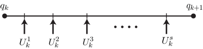
Figure 2. Internal-stage controls $\{U_{k}^{i}\}_{i=1}^{s}$ in the discrete time intervals between $k$ and $k+1$.

The following example shows that the standard Bellman equation (6.8) follows as a special case:

Example 7.2 (The standard Bellman equation).

Let $s=1$, and select

$$\Psi_{1}(\tau)=1,\qquad b_{1}=1,\qquad c^{1}=0.$$

Then, we have $B_{1}=1$, $A^{1}_{1}=0$, and $M^{1}_{1}=1$. Hence, Eq. (7.3) gives $Q^{1}=q_{k}$ (we set the endpoints $(q_{0},q_{1})$ to be $(q_{k},q_{k+1})$ here), and Eq. (7.4b) gives

$$w^{1}=f(q_{k},U_{k}^{1}).$$

However, the control $U_{k}^{1}$ is defined as follows (we shift the time intervals from $[0,h]$ to $[t_{k},t_{k}+h]$ here):

$$U_{k}^{1}\mathrel{\mathop{:}}=u(t_{k}+c^{1}h)=u(t_{k})=\mathrel{\mathop{:}}u_{k}.$$

So, we have $w^{1}=f(q_{k},u_{k})$, and thus, Eqs. (7.7) and (7.8) give

$$f_{\rm d}(q_{k},u_{k})=q_{k}+h\,f(q_{k},u_{k}),$$

and

$$C_{\rm d}(q_{k},u_{k})=h\,C(q_{k},u_{k}),$$

respectively. Notice that this approximation gives the forward-Euler discretization of the Standard Continuous-Time Optimal Control Problem 7.1 to yield the Standard Discrete Optimal Control Problem 6.1. In fact, the Bellman equation with internal-stage controls, Eq. (7.10), reduces to the standard Bellman equation (6.8):

$$\min_{u_{k}}\!\left[J_{\rm d}^{k+1}(f_{\rm d}(q_{k},u_{k}))+C_{\rm d}(q_{k},u_{k})\right]=J_{\rm d}^{k}(q_{k}).$$ (7.11)

Remark 7.3.

Higher-order approximations with any number of $s$ are possible as long as Eq. (7.4b) is solvable for $w$. See Leok and Zhang [26] for various different choices of discretizations.

7.5. Application to the Heisenberg System

Let us now apply the above results to a simple optimal control problem to illustrate the result:

Example 7.4 (The Heisenberg system; see, e.g., Brockett [8] and Bloch [7]).

Consider the following optimal control problem: For a fixed time $T>0$,

$$\min_{u(\cdot),\,v(\cdot)}\int_{0}^{T}\frac{1}{2}(u^{2}+v^{2})\,dt,$$

subject to the constraint,

$$\dot{x}=u,\qquad\dot{y}=v,\qquad\dot{z}=uy-vx.$$

This is the Standard Continuous-Time Optimal Control Problem 7.1 with $V=\mathbb{R}^{3}$, $\mathcal{U}=\mathbb{R}^{2}$, $q=(x,y,z)$, and

$$f(x,y,z,u,v)=\begin{pmatrix}u\\ v\\ uy-vx\end{pmatrix},\qquad C(x,y,z,u,v)=\frac{1}{2}(u^{2}+v^{2}).$$

If we apply the choice of the discretization in Example 7.2, we have the standard Bellman equation

$$\min_{u_{k},v_{k}}\!\left[S_{\rm d}^{k+1}(f_{\rm d}(q_{k},u_{k},v_{k}))-C_{\rm d}(q_{k},u_{k},v_{k})\right]-S_{\rm d}^{k}(q_{k})=0,$$

with $q_{k}\mathrel{\mathop{:}}=(x_{k},y_{k},z_{k})$, where

$$f_{\rm d}(q_{k},u_{k},v_{k})=\begin{pmatrix}x_{k}+h\,u_{k}\\ y_{k}+h\,v_{k}\\ z_{k}+h\,(u_{k}y_{k}-v_{k}x_{k})\end{pmatrix},\qquad C_{\rm d}(q_{k},u_{k},v_{k})=\frac{h}{2}(u_{k}^{2}+v_{k}^{2}).$$

Now, if we choose $s=2$, and select

$$(\Psi_{1}(\tau),\Psi_{2}(\tau))=(1,\cos(\pi\tau)),\qquad b=(b_{1},b_{2})=\!\left(\frac{1}{2},\frac{1}{2}\right),\qquad c=(c^{1},c^{2})=(0,1).$$

Then, we have

$$B=(B_{1},B_{2})=(1,0),\qquad A=\begin{pmatrix}0&0\\ 1&0\end{pmatrix},\qquad M=\begin{pmatrix}1&1\\ 1&-1\end{pmatrix}.$$

Leok and Zhang [26, Example 4.4] show that this choice of discretization corresponds to the Störmer–Verlet method (see, e.g., Marsden and West [30]). The Bellman equation with internal-stage controls, Eq. (7.10), then becomes

$$\min_{u_{k}^{1},v_{k}^{1},u_{k}^{2},v_{k}^{2}}\!\left[J_{\rm d}^{k+1}\!\left(f_{\rm d}\!\left(q_{k},u_{k}^{1},v_{k}^{1},u_{k}^{2},v_{k}^{2}\right)\right)+C_{\rm d}\!\left(q_{k},u_{k}^{1},v_{k}^{1},u_{k}^{2},v_{k}^{2}\right)\right]=J_{\rm d}^{k}(q_{k}),$$

where

$$f_{\rm d}\!\left(q_{k},u_{k}^{1},v_{k}^{1},u_{k}^{2},v_{k}^{2}\right)=\begin{pmatrix}x_{k}+h\,(u_{k}^{1}+u_{k}^{2})/2\vskip 6.0pt plus 2.0pt minus 2.0pt\\ y_{k}+h\,(v_{k}^{1}+v_{k}^{2})/2\vskip 6.0pt plus 2.0pt minus 2.0pt\\ \displaystyle z_{k}+h\!\left(\frac{u_{k}^{1}+u_{k}^{2}}{2}\,y_{k}-\frac{v_{k}^{1}+v_{k}^{2}}{2}\,x_{k}+\frac{u_{k}^{2}v_{k}^{1}-u_{k}^{1}v_{k}^{2}}{4}\right)\end{pmatrix},$$

and

$$C_{\rm d}\!\left(q_{k},u_{k}^{1},v_{k}^{1},u_{k}^{2},v_{k}^{2}\right)=\frac{h}{2}\!\left[\frac{(u_{k}^{1})^{2}+(u_{k}^{2})^{2}}{2}+\frac{(v_{k}^{1})^{2}+(v_{k}^{2})^{2}}{2}\right].$$

8. Conclusion and Future Work

We developed a discrete-time analogue of Hamilton–Jacobi theory starting from the discrete variational Hamiltonian mechanics formulated by Lall and West [23]. We reinterpreted and extended the discrete Hamilton–Jacobi equation given by Elnatanov and Schiff [13] in the language of discrete mechanics. Furthermore, we showed that the discrete Hamilton–Jacobi equation reduces to the discrete Riccati equation with a quadratic Hamiltonian, and also that it specializes to the Bellman equation of dynamic programming if applied to standard discrete optimal control problems. These results are discrete analogues of the corresponding known results in the continuous-time theory. Application to discrete optimal control also revealed that the Discrete Hamilton–Jacobi Theorem 4.1 specializes to a well-known result in discrete optimal control theory. We also used a Galerkin-type approximation to derive Galerkin discrete control Hamiltonians. This technique gave an explicit formula for discrete control Hamiltonians in terms of the constructs in the original continuous-time optimal control problem. By viewing the Bellman equation as a special case of the discrete Hamilton–Jacobi equation, we could introduce the discretization technique for discrete Hamiltonian mechanics into the discrete optimal control setting; this lead us to a class of Bellman equations with controls at internal stages.

We are interested in the following topics for future work:

• Application to integrable discrete systems: Theorem 4.1 gives a discrete analogue of the theory behind the technique of solution by separation of variables, i.e., the theorem relates a solution of the discrete Hamilton–Jacobi equations with that of the discrete Hamilton’s equations. An interesting question then is whether or not separation of variables applies to integrable discrete systems, e.g., discrete rigid bodies of Moser and Veselov [31] and various others discussed by Suris [33, 34].

• Development of numerical methods based on the discrete Hamilton–Jacobi equation: Hamilton–Jacobi equation has been used to develop structured integrators for Hamiltonian systems. Ge and Marsden [14] developed a numerical method that preserves momentum maps and Poisson brackets of Lie–Poisson systems by solving the Lie–Poisson Hamilton–Jacobi equation approximately. See also Channell and Scovel [11] (and references therein) for a survey of structured integrators based on the Hamilton–Jacobi equation. The present theory, being inherently discrete in time, potentially provides a variant of such numerical methods.

• Extension to discrete nonholonomic and Dirac mechanics: The present work is concerned only with unconstrained systems. Extensions to nonholonomic and Dirac mechanics, more specifically discrete-time versions of the nonholonomic Hamilton–Jacobi theory [19; 12; 32; 10] and Dirac Hamilton–Jacobi theory [27], are another direction for future research.

• Relation to the power method and iterations on the Grassmannian manifold: Ammar and Martin [2] established links between the power method, iterations on the Grassmannian manifold, and the Riccati equation. The discussion on iterations of Lagrangian subspaces and its relation to the Riccati equation in Sections 5.1 and A.2 is a special case of such links. On the other hand, Proposition 5.4 suggests that the discrete Hamilton–Jacobi equation is a generalization of the Riccati equation. We are interested in exploring possible further links implied by the generalization.

• Galerkin discrete optimal control problems: The Galerkin discrete control Hamiltonians may be considered to be a means of formulating discrete optimal control problems with higher-order of approximation to a continuous-time optimal control problem. This idea generalizes the Runge–Kutta discretizations of optimal control problems (see, e.g., Hager [18] and references therein). In fact, Leok and Zhang [26] showed that their method recovers the SPRK (symplectic-partitioned Runge–Kutta) method. Therefore, this approach is expected to provide structure-preserving higher-order numerical methods for optimal control problems.

Appendix A Discrete Linear Hamiltonian Systems

A.1. Discrete Linear Hamiltonian Systems

Suppose that the configuration space $Q$ is an $n$-dimensional vector space, and that the discrete Hamiltonian $H_{\rm d}^{+}$ or $H_{\rm d}^{-}$ is quadratic as in Eq. (5.1). Also assume that the corresponding discrete Hamiltonian map $\tilde{F}_{L_{\rm d}}:(q_{k},p_{k})\mapsto(q_{k+1},p_{k+1})$ is invertible. Then, the discrete Hamilton’s equations (2.12) or (2.15) reduce to the discrete linear Hamiltonian system

$$z_{k+1}=A_{L_{\rm d}}z_{k},$$ (A.1)

where $z_{k}\in\mathbb{R}^{2n}$ is a coordinate expression for $(q_{k},p_{k})\in Q\oplus Q^{*}$ and $A_{L_{\rm d}}:Q\oplus Q^{*}\to Q\oplus Q^{*}$ is the matrix representation of the map $\tilde{F}_{L_{\rm d}}$ under the same basis. Since $\tilde{F}_{L_{\rm d}}$ is symplectic, $A_{L_{\rm d}}$ is an $2n\times 2n$ symplectic matrix, i.e.,

$$A_{L_{\rm d}}^{T}\mathbb{J}A_{L_{\rm d}}=\mathbb{J},$$ (A.2)

where the matrix $\mathbb{J}$ is defined by

$$\mathbb{J}\mathrel{\mathop{:}}=\begin{pmatrix}0&I\\ -I&0\end{pmatrix}$$

with $I$ the $n\times n$ identity matrix.

A.2. Lagrangian Subspaces and Lagrangian Affine Spaces

Let us recall the definition of a Lagrangian subspace:

Definition A.1.

Let $V$ be a symplectic vector space with the symplectic form $\Omega$. A subspace $\mathcal{L}$ of $V$ is said to be Lagrangian if $\Omega(v,w)=0$ for any $v,w\in\mathcal{L}$ and $\dim\mathcal{L}=\dim V/2$.

We introduce the following definition for later convenience:

Definition A.2.

A subset $\tilde{\mathcal{L}}_{b}$ of a symplectic vector space $V$ is called a Lagrangian affine space if $\tilde{\mathcal{L}}_{b}=b+\mathcal{L}$ for some element $b\in V$ and a Lagrangian subspace $\mathcal{L}\subset V$.

The following fact is well-known (see, e.g., Jurdjevic [22, Theorem 6 on p. 417]):

Proposition A.3.

Let $\mathcal{L}$ be a Lagrangian subspace of $V$ and $\Phi:V\to V$ be a symplectic transformation. Then, for any $k\in\mathbb{N}$, the image of $\mathcal{L}$ under the $k$-fold composition of $\Phi$, i.e.,

$$\Phi^{k}(\mathcal{L})=\underbrace{\Phi\circ\dots\circ\Phi}_{k}(\mathcal{L})$$

is also a Lagrangian subspace of $V$.

A similar result holds for Lagrangian affine spaces:

Proposition A.4.

Let $\tilde{\mathcal{L}}_{b}=b+\mathcal{L}$ be a Lagrangian affine space of $V$ and $\Phi:V\to V$ be a symplectic transformation. Then $\Phi^{k}(\tilde{\mathcal{L}}_{b})$ is also a Lagrangian affine space of $V$ for any $k\in\mathbb{N}$. More explicitly, we have

$$\Phi^{k}(\tilde{\mathcal{L}}_{b})=\Phi^{k}b+\Phi^{k}(\mathcal{L}).$$

Proof.

Follows from a straightforward calculation. ∎

A.3. Generating Functions

Now, consider the case where $V=Q\oplus Q^{*}$ to apply the results from Section A.2 to the setting in Section A.1. This is a symplectic vector space with the symplectic form $\Omega:(Q\oplus Q^{*})\times(Q\oplus Q^{*})\to\mathbb{R}$ defined by

$$\Omega:(v,w)\mapsto v^{T}\mathbb{J}w.$$

The key result here regarding Lagrangian subspaces on $Q\oplus Q^{*}$ is the following:

Proposition A.5.

A Lagrangian subspace of $Q\oplus Q^{*}$ that is transversal to $\{0\}\oplus Q^{*}$ is the graph of an exact one-form on $Q$, i.e., $\mathcal{L}=\mathop{\mathrm{graph}}\nolimits dS$ for some function $S:Q\to\mathbb{R}$ which has the form

$$S(q)=\frac{1}{2}\left\langle Aq,q\right\rangle+C$$ (A.3)

with some symmetric linear map $A:Q\to Q^{*}$ and an arbitrary real scalar constant $C$. Moreover, the correspondence between the Lagrangian subspaces and such functions (modulo the constant term) is one-to-one.

Proof.

First, recall that a Lagrangian submanifold of $T^{*}Q$ that projects diffeomorphically onto $Q$ is the graph of a closed one-forms on $Q$ (see Abraham and Marsden [1, Proposition 5.3.15 and the subsequent paragraph on p. 410]). In our case, $Q$ is a vector space, and so the cotangent bundle $T^{*}Q$ is identified with the direct sum $Q\oplus Q^{*}$. Now, a Lagrangian subspace of $Q\oplus Q^{*}$ that is transversal to $\{0\}\oplus Q^{*}$ projects diffeomorphically onto $Q$, and so is the graph of a closed one-form. Then, by the Poincaré lemma, it follows that any such Lagrangian subspace $\mathcal{L}$ is identified with the graph of an exact one-form $dS$ with some function $S$ on $Q$, i.e., $\mathcal{L}=\mathop{\mathrm{graph}}\nolimits dS$.

However, as shown in, e.g., Jurdjevic [22, Theorem 3 on p. 233], the space of Lagrangian subspaces that are transversal to $\{0\}\oplus Q^{*}$ is in one-to-one correspondence with the space of all symmetric maps $A:Q\to Q^{*}$, with the correspondence given by $\mathcal{L}=\mathop{\mathrm{graph}}\nolimits A$. Hence, $\mathop{\mathrm{graph}}\nolimits dS=\mathop{\mathrm{graph}}\nolimits A$, or more specifically,

$$dS(q)=A_{ij}q^{j}\,dq^{i}.$$

This implies that $S$ has the form

$$S(q)=\frac{1}{2}A_{ij}q^{i}q^{j}+C,$$

with an arbitrary real scalar constant $C$. ∎

Corollary A.6.

Let $\tilde{\mathcal{L}}_{z_{0}}=z_{0}+\mathcal{L}$ be a Lagrangian affine space, where $z_{0}=(q_{0},p_{0})$ is an element in $Q\oplus Q^{*}$ and $\mathcal{L}$ is a Lagrangian subspace of $Q\oplus Q^{*}$ that is transversal to $\{0\}\oplus Q^{*}$. Then, $\tilde{\mathcal{L}}_{z_{0}}$ is the graph of an exact one-form $d\tilde{S}$ with a function $\tilde{S}:Q\to\mathbb{R}$ of the form

$$\tilde{S}(q)=\frac{1}{2}\left\langle Aq,q\right\rangle+\left\langle p_{0}-Aq_{0},q\right\rangle+C,$$ (A.4)

with some symmetric linear map $A:Q\to Q^{*}$ and an arbitrary real scalar constant $C$.

Proof.

From Proposition A.5, there exists a function $S:Q\to\mathbb{R}$ of the form Eq. (A.3) with some symmetric linear map $A:Q\to Q^{*}$ such that $\mathcal{L}=\mathop{\mathrm{graph}}\nolimits dS=\mathop{\mathrm{graph}}\nolimits A$. Let us define $\tilde{S}:Q\to R$ by

$$\tilde{S}(q)\mathrel{\mathop{:}}=S(q-q_{0})+\left\langle p_{0},q\right\rangle,$$

from which Eq. (A.4) follows by direct calculation. Then,

$$d\tilde{S}(q)=A(q-q_{0})+p_{0}.$$

and thus

$$\mathop{\mathrm{graph}}\nolimits d\tilde{S} =\{(q,d\tilde{S}(q))\ |\ q\in Q\}$$

$$=\left\{\!\left(q,A(q-q_{0})+p_{0}\right)\ |\ q\in Q\right\}$$

$$=(q_{0},p_{0})+\left\{\!\left(q-q_{0},A(q-q_{0})\right)\ |\ q\in Q\right\}$$

$$=z_{0}+\mathop{\mathrm{graph}}\nolimits A$$

$$=z_{0}+\mathcal{L}$$

$$=\tilde{\mathcal{L}}_{z_{0}}.\qed$$

References

• Abraham and Marsden [1978] R. Abraham and J. E. Marsden. Foundations of Mechanics. Addison–Wesley, 2nd edition, 1978.
• Ammar and Martin [1986] G. Ammar and C. Martin. The geometry of matrix eigenvalue methods. Acta Applicandae Mathematicae, 5(3):239–278, 1986.
• Arnold [1989] V. I. Arnold. Mathematical Methods of Classical Mechanics. Springer, 1989.
• Bellman [1971] R. Bellman. Introduction to the Mathematical Theory of Control Processes, volume 2. Academic Press, 1971.
• Bellman [1972] R. Bellman. Dynamic programming. Princeton University Press, 1972.
• Bertsekas [2005] D. P. Bertsekas. Dynamic Programming and Optimal Control, volume 1. Athena Scientific, 2005.
• Bloch [2003] A. M. Bloch. Nonholonomic Mechanics and Control. Springer, 2003.
• Brockett [1981] R. W. Brockett. Control theory and singular Riemannian geometry. In P. J. Hilton and G. S. Young, editors, New Directions in Applied Mathematics, pages 11–27. Springer, 1981.
• Cadzow [1970] J. A. Cadzow. Discrete calculus of variations. International Journal of Control, 11(3):393–407, 1970.
• Cariñena et al. [2010] J. F. Cariñena, X. Gracia, G. Marmo, E. Martínez, M. C. Munõz Lecanda, and N. Román-Roy. Geometric Hamilton–Jacobi theory for nonholonomic dynamical systems. International Journal of Geometric Methods in Modern Physics, 7(3):431–454, 2010.
• Channell and Scovel [1990] P. J. Channell and C. Scovel. Symplectic integration of Hamiltonian systems. Nonlinearity, 3(2):231–259, 1990.
• de León et al. [2010] M. de León, J. C. Marrero, and D. Martín de Diego. Linear almost Poisson structures and Hamilton–Jacobi equation. Applications to nonholonomic mechanics. Journal of Geometric Mechanics, 2(2):159–198, 2010.
• Elnatanov and Schiff [1996] N. A. Elnatanov and J. Schiff. The Hamilton–Jacobi difference equation. Functional Differential Equations, 3(279–286), 1996.
• Ge and Marsden [1988] Z. Ge and J. E. Marsden. Lie–Poisson Hamilton–Jacobi theory and Lie–Poisson integrators. Physics Letters A, 133(3):134–139, 1988.
• Gelfand and Fomin [2000] I. M. Gelfand and S. V. Fomin. Calculus of Variations. Dover, 2000.
• Goldstein et al. [2001] H. Goldstein, C. P. Poole, and J. L. Safko. Classical Mechanics. Addison Wesley, 3rd edition, 2001.
• Guibout and Bloch [2004] V. Guibout and A. M. Bloch. A discrete maximum principle for solving optimal control problems. In 43rd IEEE Conference on Decision and Control, volume 2, pages 1806–1811 Vol.2, 2004.
• Hager [2000] W. W. Hager. Runge–Kutta methods in optimal control and the transformed adjoint system. Numerische Mathematik, 87(2):247–282, 2000.
• Iglesias-Ponte et al. [2008] D. Iglesias-Ponte, M. de León, and D. Martín de Diego. Towards a Hamilton–Jacobi theory for nonholonomic mechanical systems. Journal of Physics A: Mathematical and Theoretical, 41(1), 2008.
• Jalnapurkar et al. [2006] S. M. Jalnapurkar, M. Leok, J. E. Marsden, and M. West. Discrete Routh reduction. Journal of Physics A: Mathematical and General, 39(19):5521–5544, 2006.
• Jordan and Polak [1964] B. W. Jordan and E. Polak. Theory of a class of discrete optimal control systems. Journal of Electronics and Control, 17:694–711, 1964.
• Jurdjevic [1997] V. Jurdjevic. Geometric control theory. Cambridge University Press, Cambridge, 1997.
• Lall and West [2006] S. Lall and M. West. Discrete variational Hamiltonian mechanics. Journal of Physics A: Mathematical and General, 39(19):5509–5519, 2006.
• Lanczos [1986] C. Lanczos. The Variational Principles of Mechanics. Dover, 4th edition, 1986.
• Leok [2004] M. Leok. Foundations of Computational Geometric Mechanics. PhD thesis, California Institute of Technology, 2004.
• Leok and Zhang [2011] M. Leok and J. Zhang. Discrete Hamiltonian variational integrators. IMA Journal of Numerical Analysis, 2011.
• [27] M. Leok, T. Ohsawa, and D. Sosa. Hamilton–Jacobi theory for degenerate Lagrangian systems with constraints. in preparation.
• Leok et al. [2004] M. Leok, J. E. Marsden, and A. Weinstein. A discrete theory of connections on principal bundles. Preprint, 2004.
• Marsden and Ratiu [1999] J. E. Marsden and T. S. Ratiu. Introduction to Mechanics and Symmetry. Springer, 1999.
• Marsden and West [2001] J. E. Marsden and M. West. Discrete mechanics and variational integrators. Acta Numerica, pages 357–514, 2001.
• Moser and Veselov [1991] J. Moser and A. P. Veselov. Discrete versions of some classical integrable systems and factorization of matrix polynomials. Communications in Mathematical Physics, 139(2):217–243, 1991.
• Ohsawa and Bloch [2009] T. Ohsawa and A. M. Bloch. Nonholonomic Hamilton–Jacobi equation and integrability. Journal of Geometric Mechanics, 1(4):461–481, 2009.
• Suris [2003] Y. B. Suris. The problem of integrable discretization: Hamiltonian approach. Birkhäuser, Basel, 2003.
• Suris [2004] Y. B. Suris. Discrete Lagrangian models. In Discrete Integrable Systems, volume 644 of Lecture Notes in Physics, pages 111–184. Springer, 2004.