Cosmic Evolution of Virial and Stellar Mass in Massive Early-Type Galaxies 111Based on observations with the NASA/ESA Hubble Space Telescope obtained at the Space Telescope Science Institute, which is operated by the Association of Universities for Research in Astronomy, Incorporated, under NASA contract NAS5-26555.
Abstract
We measure the average mass properties of a sample of 41 strong gravitational lenses at moderate redshift (z 0.4 – 0.9), and present the lens redshift for 6 of these galaxies for the first time. Using the techniques of strong and weak gravitational lensing on archival data obtained from the Hubble Space Telescope, we determine that the average mass overdensity profile of the lenses can be fit with a power-law profile () that is within 1- of an isothermal profile () with velocity dispersion = 260 20 km s-1. Additionally, we use a two-component de Vaucouleurs+NFW model to disentangle the total mass profile into separate luminous and dark matter components, and determine the relative fraction of each component. We measure the average rest frame V-band stellar mass-to-light ratio () and virial mass-to-light ratio () for our sample, resulting in a virial-to-stellar mass ratio of . Relaxing the NFW assumption, we estimate that changing the inner slope of the dark matter profile by 20% yields a 30% change in stellar mass-to-light ratio. Finally, we compare our results to a previous study using low redshift lenses, to understand how galaxy mass profiles evolve over time. We investigate the evolution of , and find best fit parameters of and , constraining the growth of virial to stellar mass ratio over the last 7 Gigayears. We note that, by using a sample of strong lenses, we are able to constrain the growth of without making any assumptions about the IMF of the stellar population.
Subject headings:
dark matter – gravitational lensing – galaxies: elliptical and lenticular, cD – galaxies: evolution – galaxies: structure1. Introduction
Observations over the last few decades have suggested that galaxies are embedded in an extended, diffuse halo of dark matter (e.g. Peterson et al., 1978; White & Rees, 1978; Rubin et al., 1979; Blumenthal et al., 1984), which contributes up to 95 percent of the total mass (Hoekstra et al., 2005; Jiang & Kochanek, 2007; Avila-Reese et al., 2008). Because of the overwhelming fraction of dark matter, numerical simulations dealing with the formation and assembly of galaxy mass often focus on dark matter alone (e.g., the Via Lactea Simulation; Kuhlen et al., 2008), and these simulations have made very specific predictions about the overall profile of galaxy-sized mass distributions (e.g., Navarro et al., 1997; Moore et al., 1998; Jing, 2000; Stoehr, 2006; Diemand et al., 2007; Schmidt et al., 2008). However, when compared to observations, these simulations often fail to accurately recreate the observed shape of galaxy mass profiles (Salucci, 2001; Gentile et al., 2004; Simon et al., 2005; Gentile et al., 2007; Kuzio de Naray et al., 2008; Seigar et al., 2008; Sand et al., 2008). This disagreement is attributed largely to the complex physics of baryon interaction (e.g. frictional dissipation and radiative cooling) which is still not well understood and is difficult to model.
There are many possible methods capable of measuring the distribution of matter on small ( 1 Mpc) scales, and techniques used for characterizing a radial mass profile include measuring the rotation curves from planetary nebulae (Romanowsky et al., 2003; Arnaboldi et al., 2004; Merrett et al., 2006; de Lorenzi et al., 2008; Napolitano et al., 2009), kinematics of stellar populations (Bertin et al., 1994; Cappellari et al., 2006; van der Wel & van der Marel, 2008) and H I gas (Uson & Matthews, 2003; Jackson et al., 2004; Andersen et al., 2006; Matthews & Uson, 2008), or the temperature of X-ray emitting gas (Humphrey et al., 2006; Churazov et al., 2008).
In this paper, we use a powerful alternative technique: gravitational lensing (e.g., Brainerd et al., 1996; Fischer et al., 2000; Wilson et al., 2001; Kleinheinrich et al., 2006; Parker et al., 2007). The power of lensing is due to the fact that the technique is able to directly trace the total mass (luminous + non-luminous) enclosed within a given radius without needing to make any assumptions about the dynamical state of the mass in question. In addition, lensing does not rely on the presence of kinematic tracers, which are often only visible in very low-redshift galaxies, and even then are typically not present in the outer halo regions where dark matter dominates.
Furthermore, since we analyze a sample of strong lenses, we are able to combine the mass constraints determined from both strong lensing and weak lensing. This allows us to probe the total mass distribution over a much wider range of physical distances than by using weak lensing alone, and also allows us to constrain the properties of stellar mass distribution without selecting a specific stellar initial mass function (IMF). Instead, we rely on directly-derived properties: lensing-inferred mass and total luminosity (although we do make an assumption about the shape of the dark matter halo).
For early-type galaxies, several lensing-based studies have shown the typical shape of the mass density profile to be consistent with an isothermal () model, given the uncertainties on the measurements, between distances of kpc (Sheldon et al., 2004; Mandelbaum et al., 2006). However, due to the low signal-to-noise ratio (SNR) on the lensing signal obtained from an individual galaxy, these studies rely on stacking a large number of galaxies into a single sample to determine the average profile of the entire stack. For this work, we utilize deep imaging from the Hubble Space Telescope (HST). In general, space-based data will have a much higher density of background galaxies () when compared to data taken from the ground over an identical exposure time. This increased background density count not only enables us to detect a weak lensing signal much closer to the center of the lensing galaxy, but also allows for a significant detection with fewer stacked galaxies (), because the expected weak lensing SNR scales as . The ability to work on a small sample size is particularly useful, given the relative paucity of known strong lenses at all redshifts.
In this work, we are able to extend the results of Gavazzi et al. (2007, hereafter G07), who conducted a similar mass profile study on a small (22 lens) sample of low redshift (z 0.2) early-type strong gravitational lenses collected from the Sloan Lens ACS Survey (SLACS; see e.g. Bolton et al., 2006, 2008) over a wide range of physical distances ( kpc). From this work, it was shown that, like their non lensing counterparts, the total mass density profile of strong lensing ellipticals could be described by a roughly isothermal model (although they note that the comparison between the data and the model was done without a formal fit). This was thought to be due to the combination of baryonic and dark matter, the so-called Bulge-Halo Conspiracy, in which a relatively steep luminous matter profile and a shallower dark matter profile combine in such a way that the total mass distribution of the galaxy can be well approximated by an isothermal model (Treu et al., 2006). By comparing this data set to our moderate redshift sample, we thus explore the evolutionary trends of massive early-type galaxies.
This paper is organized as follows: In Section 2, we describe our lens sample, the lens selection criteria, and the data reduction pipeline used for this work. At this point, the interested reader may turn to the appendix, where we describe our techniques for analyzing weak lensing shear, paying specific attention to signal to noise optimization and the removal of systematic errors. In Section 3, we use a two-component model to determine the contributions of the stellar and dark matter components to the total profile. We present all of our results in Section 4, the reader interested in the science may skip directly to this section. We discuss the results and compare them to the SLACS results in Section 5, looking for evolutionary differences between the samples. Finally, we summarize our results in Section 6.
Throughout this work, we assume a flat cosmology with km s-1 Mpc-1, , and . All magnitudes presented in this paper are AB magnitudes.
2. Data
2.1. Imaging Data
For this analysis, we focus on a sample of 41 strong gravitational lenses at moderate redshift (). A majority of the sample was observed as part of the CASTLES program222http://cfa-www.harvard.edu/castles/, but it also contains lenses found in the COSMOS survey333http://cosmos.astro.caltech.edu/ (Faure et al., 2008) and the Extended Groth Strip (Moustakas et al., 2007), as well as targeted exposures of individual lens systems. Unlike other data sets that have been selected in some uniform way (such as the SLACS lenses), our lens sample is drawn from a variety of sources and selected simply for being lenses with early-type morphologies in the desired redshift range. However, we do note that systems known to be strongly affected by the presence of a galaxy cluster (Q0957+561, SDSS1004+4112, and B2108+213) were excluded from the sample. A full list of the lenses can be seen in Table 1.
| Lens Name | Program | Exp. Time | a,ba,bfootnotemark: | bbFor the COSMOS lenses, redshift values with 3 significant figures were determined spectroscopically, and redshift values with 2 significant figures are determined photometrically, according to the catalog of Ilbert et al. (2009). | cc is the weight value associated with each lens field, described in the appendix. | References | ||
|---|---|---|---|---|---|---|---|---|
| ID | () | ( Mpc) | ( pc-2) | |||||
| B0218+357 | 9450 | 4320.0 | 0.68 | 0.96 | 1020 | 0.320 | 5097 | [1],[2],[3] |
| SDSS0246-0825 | 9744 | 2288.0 | 0.724 | 1.68 | 1045 | 0.293 | 5035 | [4] |
| CFRS03P1077 | 9744 | 2296.0 | 0.938 | 2.941 | 1137 | 0.188 | 8965 | [5] |
| HE0435-1223 | 9744 | 1445.0 | 0.454 | 1.689 | 842 | 0.486 | 3702 | [6],[7] |
| B0445+128 | 9744 | 5228.0 | 0.557 | 931 | 0.406 | 3969 | [8] | |
| B0631+519 | 9744 | 2446.0 | 0.62 | 979 | 0.360 | 4267 | [9] | |
| J0816+5003 | 9744 | 2440.0 | 825 | 0.500 | 3678 | [10] | ||
| B0850+054 | 9744 | 2296.0 | 0.59 | 3.93 | 957 | 0.381 | 4112 | [11] |
| SDSS0903+5028 | 9744 | 2444.0 | 0.388 | 3.605 | 761 | 0.552 | 3645 | [12] |
| SDSS0924+0219 | 9744 | 2296.0 | 0.394 | 1.524 | 763 | 0.550 | 3644 | [13],[14] |
| J1004+1229 | 9744 | 2296.0 | 0.95 | 2.65 | 1141 | 0.183 | 9397 | [15] |
| HE1113-0641 | 9744 | 1062.0 | 0.75 | 1.235 | 1059 | 0.278 | 5298 | [16] |
| Q1131-1231 | 9744 | 1980.0 | 0.295 | 0.658 | 635 | 0.646 | 3803 | [17] |
| SDSS1138+0314 | 9744 | 2296.0 | 0.45 | 2.44 | 831 | 0.495 | 3685 | [18],[19] |
| SDSS1155+6346 | 9744 | 1748.0 | 0.176 | 2.89 | 430 | 0.780 | 4782 | [20] |
| SDSS1226-0006 | 9744 | 2296.0 | 0.52 | 1.12 | 899 | 0.435 | 3841 | [18],[19] |
| B1608+656 | 10158 | 9744.0 | 0.63 | 1.39 | 987 | 0.353 | 4774 | [21],[22] |
| WFI2033-4723 | 9744 | 2085.0 | 0.66 | 1.66 | 1007 | 0.333 | 4516 | [18],[23] |
| COSMOS5857+5949 | 9822 | 2028.0 | 0.39 | 763 | 0.550 | 3646 | [24] | |
| COSMOS5914+1219 | 9822 | 2028.0 | 1.13 | 1169 | 0.148 | 15755 | [24] | |
| COSMOS5921+0638 | 9822 | 2028.0 | 0.551 | 3.15 | 926 | 0.411 | 3948 | [24],[25] |
| COSMOS5941+3628 | 9822 | 2028.0 | 0.88 | 1124 | 0.204 | 7834 | [24] | |
| COSMOS5947+4752 | 10092 | 2028.0 | 0.345 | 706 | 0.595 | 3681 | [24],[26] | |
| COSMOS0012+2015 | 9822 | 2028.0 | 0.378 | 749 | 0.562 | 3649 | [24],[26] | |
| COSMOS0013+2249 | 9822 | 2028.0 | 0.346 | 707 | 0.594 | 3680 | [24],[26] | |
| COSMOS0018+3845 | 9822 | 2028.0 | 0.71 | 1037 | 0.301 | 4908 | [24] | |
| COSMOS0038+4133 | 10092 | 2028.0 | 0.738 | 1121 | 0.208 | 7583 | [24],[29] | |
| COSMOS0047+5023 | 9822 | 2028.0 | 0.87 | 1105 | 0.226 | 6729 | [24] | |
| COSMOS0049+5128 | 9822 | 2028.0 | 0.337 | 695 | 0.603 | 3694 | [24],[26] | |
| COSMOS0050+4901 | 10092 | 2028.0 | 0.960 | 1144 | 0.179 | 9795 | [24],[26] | |
| COSMOS0056+1226 | 9822 | 2028.0 | 0.361 | 0.81 | 727 | 0.579 | 3661 | [24],[26],[29] |
| COSMOS0124+5121 | 9822 | 2028.0 | 0.84 | 1101 | 0.231 | 6546 | [24] | |
| COSMOS0211+1139 | 9822 | 2028.0 | 0.920 | 1124 | 0.204 | 7834 | [24],[29] | |
| COSMOS0216+2955 | 9822 | 2028.0 | 0.608 | 1013 | 0.326 | 4588 | [24],[29] | |
| COSMOS0227+0451 | 10092 | 2028.0 | 0.89 | 1121 | 0.208 | 7583 | [24] | |
| COSMOS0254+1430 | 10092 | 2028.0 | 0.417 | 0.779 | 825 | 0.500 | 3678 | [24],[29] |
| J095930.93+023427.7 | 9822 | 2028.0 | 0.892 | 1122 | 0.207 | 7150 | [27],[29] | |
| J100140.12+020040.9 | 9822 | 2028.0 | 0.879 | 1117 | 0.213 | 6987 | [27],[29] | |
| “Anchor” | 10134 | 2100.0 | 0.463 | 845 | 0.483 | 3707 | [28] | |
| “Cross” | 10134 | 2100.0 | 0.810 | 3.40 | 1088 | 0.246 | 6060 | [28] |
| “Dewdrop” | 10134 | 2100.0 | 0.580 | 0.982 | 950 | 0.389 | 4068 | [28] |
Each system in the sample was chosen based on the existence of publicly available HST images, subject to the following criteria: the system needed to be observed using the Wide Field Channel (WFC) of the Advanced Camera for Surveys (ACS; Ford et al., 1998), and the total exposure needed to be at least 1800 seconds through the F814W filter. This exposure time yields background densities of 70 galaxies or more.
The imaging data for all the lenses were obtained through the Multimission Archive at STScI (MAST444http://archive.stsci.edu/), from programs G0-9744 (CASTLES: PI Kochanek), GO-9822 and 10092 (COSMOS: PI Scoville), GO-10134 (EGS: PI Davis), GO-10158 (B1608+656: PI Fassnacht), and GO-9450 (B0218+357: PI Jackson). The lens systems that had been specifically targeted by HST (B1608+656, B0218+357, and the CASTLES lenses) are located at the WF1 target point, whereas the serendipitously discovered COSMOS and EGS lenses appear at random positions in the ACS field of view.
In addition to the F814W data, some lens systems have secondary imaging in either the F555W or F606W filter. These extra data could prove to be useful in future refinements to this study, especially in using color selection to reject foreground interlopers from the population of background sources (see the appendix). However, we do not use the information in our present weak lensing analysis: a significant fraction of our sample has only F814W imaging, and for systems that do have multi-band data, the redshift/color relationship can be highly degenerate when dealing with only two filters. Thus, we do not expect significant improvement in the signal.
The raw data were processed through a reduction pipeline created for the HST Archive Galaxy-scale Gravitational Lens Survey (HAGGLeS, P.J. Marshall et al., in preperation), which we briefly describe. First, each individual raw exposure of a given lens system is calibrated, using the calacs package in STSDAS555STSDAS is a product of the Space Telescope Science Institute, which is operated by AURA for NASA, a software system built on top of IRAF666IRAF (Image Reduction and Analysis Facility) is distributed by the National Optical Astronomy Observatory, which is operated by the Association of Universities for Research in Astronomy, Inc., under cooperative agreement with the National Science Foundation.. Once calibrated, the exposures are aligned and combined into a single stacked image using multidrizzle (Koekemoer et al., 2002). Since even slight misalignments can introduce systematic errors in the weak lensing signal, the HAGGLeS pipeline refines the image alignment derived from the astrometric header by cross-correlating the positions of bright, well-defined objects (bright unsaturated stars, nebular knots in spiral galaxies, etc.) in each exposure in order to look for residual shift or rotation misalignments. These residual shifts are then fed to multidrizzle, and this process is repeated until the shift refinements become negligibly small. After final alignment and combination, the composite output image is resampled in multidrizzle from the native scale of 0.05″pixel-1 to one of 0.03″pixel-1, using the “Square” interpolation kernel. This is done primarily to better sample the ACS instrumental point-spread function (PSF). Lastly, the resampled image is registered to a common World Coordinate System using positions from the USNO-B1 catalog (Monet et al., 2003).
After processing the images, we create initial photometric galaxy catalogs for each field using SExtractor (Bertin & Arnouts, 1996). As a goal of this study is to compare our results as closely as possible to those in G07, we use their SExtractor parameter set for our analysis. The parameters can be seen in Table 2. These parameters are selected to optimize detection of a suitably high number of small, dim objects, while also deblending close neighbors. This leads to a large number of spurious detections but the “false positives” are rejected during the analysis by applying a series of cuts to the data. This procedure is discussed more fully in the appendix.
| Parameter Name | Value |
|---|---|
DETECT_MINAREA |
10 |
DETECT_THRESH |
1.1 |
DEBLEND_NTHRESH |
64 |
DEBLEND_MINCONT |
0.005 |
PHOT_AUTOPARAMS |
2.5, 3.5 |
PHOT_FLUXFRAC |
0.5 |
BACK_SIZE |
64 |
BACK_FILTERSIZE |
3 |
BACKPHOTO_TYPE |
GLOBAL |
2.2. Spectroscopic Data
While the determination of the weak lensing signal uses a generalized description of the redshift distribution of the background objects, the additional inclusion of the strong lensing information in the analysis (§3.3) is only possible if the redshifts of both the lens and the multiply-imaged background have been measured. Thus, to improve the utility of the lens sample, we obtained spectroscopic data on some of the best lens candidates from the COSMOS sample using the Low-Resolution Imaging Spectrograph (LRIS; Oke et al., 1995) on the Keck I Telescope. The observations were conducted on UT 2009 Feb 22 and 23 in good conditions, with seeing ranging from 08 to 1″. Spectra were obtained for the J095930.93+023427.7, 0038+4133, 0050+4901, 0056+1226, 0211+1139, J100140.12+020040.9, 0216+2955, and 0254+1430 lens systems, where 5930+3427, 0056+1226, J100140.12+020040.9, 0211+1139, and 0216+2955 were observed through slitmasks and the remaining systems were observed using a 1″ longslit. The exposure times were set by the F814W magnitude of the lensing galaxy and ranged from 1200 to 7200 s. The lensed source galaxies were much fainter than the lenses and, thus, the chosen exposure times were not sufficient to measure redshifts unless strong emission features or breaks in the spectrum were observed. In cases where we could not determine a redshift for the source galaxy, strong lensing constraints could not be obtained. However, these lenses are still useful for, and are included in, the weak lensing analysis. The data were reduced using custom Python scripts that performed the flat-field corrections, wavelength calibrations, rectifications, and extractions of the spectra. The extracted spectra were examined for multiple emission and/or absorption features. We were able to determine lens redshifts for six of the seven systems that were targeted (the slit for 0056+1226 was placed only over the lensed source because the lens redshift was previously known), but only two source redshifts. Thus, the new redshifts for COSMOS systems resulting from this work are: J095930.93+023427.7 (), 0038+4133 (), 0056+1226 (, based mostly on the 4000Å break), J100140.12+020040.9 (), 0211+1139 (, based mostly on the 4000Å break), 0216+2955 (), and 0254+1430 (, ).
3. Disentangling Mass and Light
After reducing the data, we perform a full weak lensing analysis on the galaxy fields to infer the average mass properties of our lenses. The interested reader can find the full details of this analysis in the appendix. To summarize however, we measure the shapes of all background galaxies, apply a series of data cuts to remove contaminants, and employ a system of tests to minimize systematic uncertainty. We then convert these galaxy shape measurements into a measure of mass overdensity as a function of radius (), which we can compare with specific models to infer other properties of the lenses. The profile reflects the total mass distribution of the lens galaxy. We can investigate the dark matter contribution by jointly modeling the luminous and dark components, constrained by the lens galaxy surface brightness profiles. To disentangle the luminous stellar mass profile from its surrounding dark matter halo, we employ a simple two-component mass model, whereby the stellar mass profile traces the light profile, and the dark profile exists as a single dark matter halo, centered on the galaxy itself (a one-halo central term in the framework of the “halo model”). This simplifying assumption explicitly excludes any mass contribution from an underlying group/cluster halo, or nearby satellite galaxies (the two-halo term), but we feel it is a well warranted assumption, because only a small fraction of massive elliptical galaxies ( 15%) are located away from the center of their host halos (Mandelbaum et al., 2006).
3.1. Luminous Component
We begin our process of modeling stellar light by using
GALFIT777http://users.ociw.edu/peng/work/galfit/galfit.html
(Peng et al., 2002) to fit a de Vaucouleurs profile (de Vaucouleurs, 1948) to the
F814W images of each strong lensing galaxy, carefully masking out any
contaminating light from nearby satellites or (more importantly) the
strongly lensed images. In most cases, this masking is achieved by
running GALFIT on a small cutout of the galaxy (typically a square 2.5
times the galaxy’s FWHM parameter – as determined by
SExtractor – on a side). Nearly all of the light from our
moderate-redshift lenses is contained well within the lensing Einstein
radius, making it possible to exclude all of the lensed background
structure without excluding significant portions of the light profile
of the foreground galaxy. In the few cases where this cutout method
is not feasible (e.g. compact 4-image quasar lenses such as
SDSS1138+0314 or HE1113-0641) we generate custom GALFIT masks to block
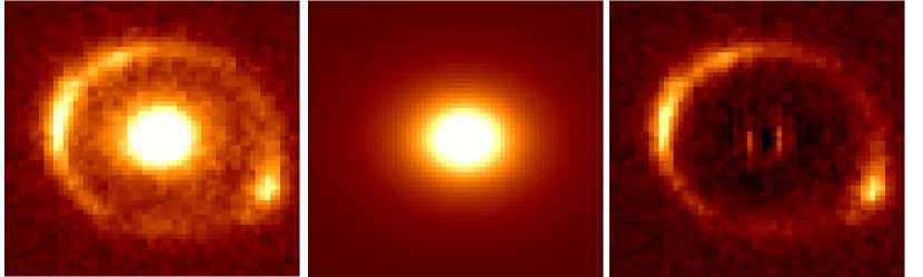
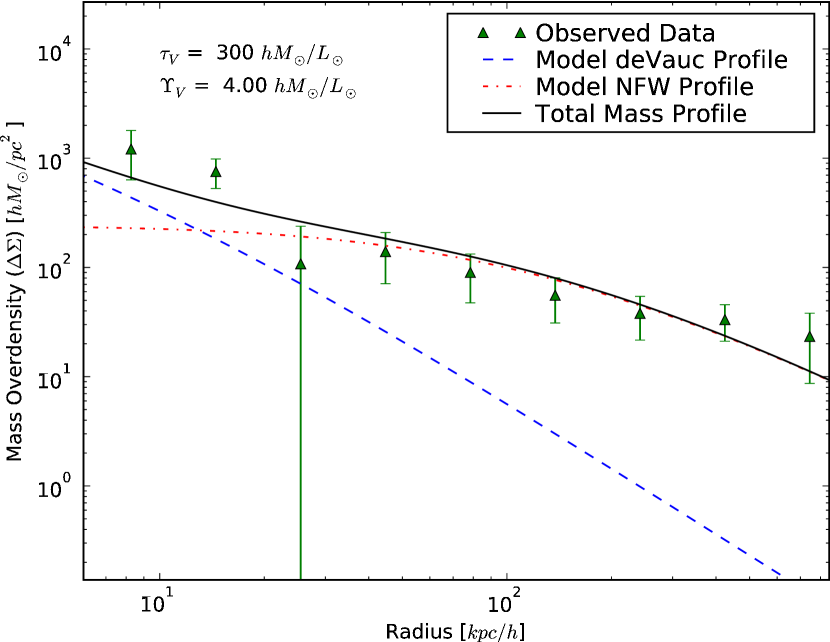
out the remaining contaminating light. An example of the GALFIT
modeling can be seen in Figure 1.
By explicitly fitting with a de Vaucouleurs profile, we obtain two parameters for each galaxy that can be used in the mass profile modeling: an effective radius () and an F814W (I-band) magnitude (). We first convert the I-band apparent magnitudes into F555W (V-band) absolute magnitudes () by calculating K-corrections using the elliptical galaxy template from the Kinney-Calzetti spectral atlas (Kinney et al., 1996), and correcting for galactic extinction using the Schlegel et al. (1998) dust maps. This is done so that we may more readily compare our results to both G07 and previous mass-to-light () studies. To homogenize the sample, we passively evolve all V-band luminosities to a fiducial redshift , using the relation (Grillo et al., 2009):
| (1) |
We also convert the total luminosity into effective surface brightness () using the equation:
| (2) |
where and are the general Sérsic parameters (for the de Vaucouleurs profile, , ). The relevant parameters obtained through the photometric modeling are in Table 3.
We model the stellar contribution to the mass profile as:
| (3) |
where is the stellar mass surface density, and is the rest-frame V-band stellar mass to light ratio (). Since both and are fixed by the GALFIT model for any given galaxy, this stellar mass profile has the benefit of being described by only a single free parameter, .
| Lens Name | mI | K-corr | E(B-V) | MV - 2.5log10() | Ie | q | PA | ||
|---|---|---|---|---|---|---|---|---|---|
| () | () | ( kpc-2) | |||||||
| B0218+357 | 0.17 | 0.37 | 19.89 | -0.19 | 0.0680 | -20.10 | 123.62 | 0.97 | 66.02 |
| SDSS0246-0825 | 0.6 | 0.99 | 19.81 | -0.10 | 0.0266 | -21.78 | 557.53 | 0.53 | 24.88 |
| CFRS03P1077 | 1.05 | 1.89 | 20.30 | 0.42 | 0.0983 | -23.46 | 54.24 | 0.66 | 32.40 |
| HE0435-1223 | 1.21 | 1.12 | 19.17 | -0.49 | 0.0590 | -21.65 | 99.52 | 0.79 | -83.16 |
| B0445+128 | 0.68 | 2.29 | 20.09 | -0.38 | 0.3837 | -21.35 | 12.94 | 0.71 | -54.21 |
| B0631+519 | 0.58 | 0.84 | 20.30 | -0.29 | 0.0890 | -21.65 | 104.31 | 0.81 | 8.35 |
| J0816+5003 | 2.5 | 0.94 | 18.54 | -0.51 | 0.0466 | -22.94 | 293.74 | 0.86 | 46.23 |
| B0850+054 | 0.34 | 0.25 | 21.73 | -0.34 | 0.0615 | -20.60 | 478.79 | 0.42 | 55.28 |
| SDSS0903+5028 | 1.5 | 0.55 | 19.34 | -0.58 | 0.0245 | -20.93 | 293.68 | 0.93 | -69.39 |
| SDSS0924+0219 | 0.88 | 0.58 | 19.38 | -0.58 | 0.0551 | -20.90 | 248.06 | 0.91 | 52.62 |
| J1004+1229 | 0.77 | 0.51 | 21.80 | 0.45 | 0.0372 | -21.88 | 165.29 | 0.38 | 64.87 |
| HE1113-0641 | 0.44 | 2.35 | 18.16 | -0.05 | 0.0386 | -21.72 | 168.03 | 0.76 | -59.19 |
| Q1131-1231 | 1.9 | 3.63 | 16.78 | -0.68 | 0.0352 | -22.71 | 55.83 | 0.78 | 10.93 |
| SDSS1138+0314 | 0.67 | 0.42 | 20.12 | -0.50 | 0.0196 | -20.60 | 286.33 | 0.79 | 7.79 |
| SDSS1155+6346 | 0.98 | 0.52 | 17.60 | -0.80 | 0.0141 | -20.48 | 898.45 | 0.59 | 36.23 |
| SDSS1226-0006 | 0.63 | 0.46 | 18.98 | -0.42 | 0.0233 | -21.32 | 230.87 | 0.28 | -34.38 |
| B1608+656 | 1.14 | 0.89 | 19.51 | -0.28 | 0.0310 | -20.24 | 26.09 | 0.44 | -13.98 |
| WFI2033-4723 | 1.17 | 0.73 | 20.25 | -0.22 | 0.0461 | -21.78 | 140.47 | 0.82 | 41.79 |
| COSMOS5857+5949 | 2.15 | 1.23 | 19.63 | -0.58 | 0.0193 | -20.67 | 45.30 | 0.60 | 58.41 |
| COSMOS5914+1219 | 1.86 | 1.27 | 22.11 | 0.75 | 0.0202 | -22.33 | 29.20 | 0.69 | -22.72 |
| COSMOS5921+0638 | 0.8 | 0.33 | 20.62 | -0.39 | 0.0205 | -20.77 | 366.25 | 0.84 | -62.64 |
| COSMOS5941+3628 | 1.21 | 0.83 | 20.90 | 0.32 | 0.0191 | -22.43 | 120.08 | 0.90 | 69.28 |
| COSMOS5947+4752 | 2.55 | 0.35 | 19.96 | -0.64 | 0.0209 | -19.97 | 365.42 | 0.89 | 89.20 |
| COSMOS0012+2015 | 0.9 | 0.51 | 19.42 | -0.59 | 0.0185 | -20.84 | 321.34 | 0.64 | 68.23 |
| COSMOS0013+2249 | 1.65 | 2.02 | 18.33 | -0.63 | 0.0178 | -21.69 | 52.91 | 0.82 | -54.76 |
| COSMOS0018+3845 | 0.4 | 0.32 | 23.13 | -0.13 | 0.0187 | -19.20 | 61.48 | 0.68 | 55.42 |
| COSMOS0038+4133 | 0.74 | 1.11 | 20.36 | 0.29 | 0.0186 | -22.31 | 82.28 | 0.74 | 88.38 |
| COSMOS0047+5023 | 0.7 | 1.33 | 20.16 | 0.19 | 0.0182 | -23.06 | 84.67 | 0.80 | -56.86 |
| COSMOS0049+5128 | 2.22 | 0.31 | 20.09 | -0.64 | 0.0182 | -19.81 | 428.99 | 0.75 | 22.46 |
| COSMOS0050+4901 | 1.9 | 0.74 | 21.21 | 0.48 | 0.0189 | -22.53 | 140.32 | 0.73 | -65.24 |
| COSMOS0056+1226 | 1.2 | 0.76 | 18.92 | -0.62 | 0.0164 | -21.16 | 210.72 | 0.90 | -61.32 |
| COSMOS0124+5121 | 0.84 | 0.27 | 22.33 | 0.17 | 0.0188 | -20.79 | 271.75 | 0.65 | 38.48 |
| COSMOS0211+1139 | 3.2 | 1.66 | 20.50 | 0.32 | 0.0168 | -23.05 | 48.23 | 0.61 | -83.30 |
| COSMOS0216+2955 | 1.96 | 0.99 | 19.98 | -0.20 | 0.0185 | -21.70 | 84.55 | 0.81 | 62.14 |
| COSMOS0227+0451 | 1.62 | 0.71 | 21.37 | 0.29 | 0.0176 | -22.05 | 112.95 | 0.60 | -10.32 |
| COSMOS0245+1430 | 1.54 | 1.70 | 18.63 | -0.51 | 0.0191 | -22.26 | 72.62 | 0.59 | 31.75 |
| J095930.93+023427.7 | 0.89 | 0.95 | 21.26 | 0.28 | 0.0191 | -22.07 | 63.99 | 0.69 | -2.33 |
| J100140.12+020040.9 | 0.79 | 0.29 | 21.71 | 0.26 | 0.0180 | -21.58 | 446.53 | 0.83 | -71.80 |
| “Anchor” | 1.1 | 0.49 | 19.88 | -0.49 | 0.0103 | -20.93 | 285.63 | 0.92 | -56.16 |
| “Cross” | 1.22 | 0.90 | 20.29 | 0.09 | 0.0085 | -22.60 | 137.47 | 0.79 | 78.92 |
| “Dewdrop” | 0.76 | 0.50 | 19.96 | -0.35 | 0.0089 | -21.59 | 314.46 | 0.85 | 79.14 |
3.2. Dark Component
For the dark matter, we assume a functional form of the Navarro, Frenk and White (NFW; Navarro et al., 1997) profile. The projected, two dimensional NFW mass density profile () can be described generally by:
| (4) |
(e.g., Wright & Brainerd, 2000), where is the NFW “scale radius”, is the critical density of the universe, and = ()/[ln() - ] is a function of the concentration parameter (). is the radius at which the total mass density is times . For each model, the value of is determined solely by the redshift of the lens galaxy using the prescription of Bryan & Norman (1998), which for our assumed cosmology allows to be considered the virial radius of the system. For galaxies at , is 140, and all galaxies in our lens sample have overdensity values between and .
By defining the virial radius, we are also able to further constrain the concentration parameter by assuming a functional form given by:
| (5) |
as found in numerical dark matter simulations (Bullock et al., 2001; Eke et al., 2001; Hoekstra et al., 2005), and where is the total virial mass. While we assume no intrinsic scatter in the mass-concentration relation for our initial analysis, we do consider the effects of scatter, as well as other systematic effects that can implicitly alter this relationship, in §5.3. Rather than attempt to constrain the virial mass for each galaxy in our sample individually, we instead choose to parameterize these masses as a function of V-band luminosity (). Specifically, we choose the form , where is defined to be the virial mass to light ratio. This then allows us to define the dark matter mass profile in terms of:
| (6) |
As in the case of the stellar mass profile, we take from the GALFIT models and, since the redshift is already known for each lens, we once again are left with a model with a single free parameter, this time .
3.3. Model Fitting
3.3.1 Mass Overdensity Models
We fit the models to the observed profile, determining the best-fit ratios associated with the lens galaxies through a minimization procedure. We compare the observed weak lensing profile to the two-component models and average over contributions from individual models in order to mimic the procedure used in the weak lensing analysis. The merit function for our procedure is:
| (7) |
where is the observed mass overdensity at radius (Table 4), is the error associated with that measurement, and and are the stellar and dark matter mass overdensity models evaluated at (using the parameters of lens ), constructed according to Equation (A12). This optimization to the weak lensing data set is performed for the full sample of lenses.
To take full advantage of our data set, we also incorporate the strong lensing information. We note that, for all strong lenses, the average value of the mass surface density within the Einstein radius is equivalent to the critical lensing density, . This can be proven by noting that for a circularly symmetric lens, the tangential reduced shear profile () can be written in the form:
| (8) |
Because is, by definition, equal to 1 at it is a simple matter to show that .
Thus, for all lenses for which we know both the lens and source galaxy redshift, we can accurately determine the value of the critical density of the system and further constrain the models. The strong lensing merit function is given by:
| (9) |
where is the actual critical density of lens i, is the uncertainty on that value, and are the stellar and dark matter average mass density models of lens , evaluated at the Einstein radius of that specific lens, and N is the number of lenses for which the source redshift has been measured.
3.3.2 Reduced Shear Models
In addition to the mass overdensity model fit described in §3.3.1, we also fit models directly to our reduced shear data. Although shear is correlated with mass overdensity, we do expect there to be a slight discrepancy between the two methods: by creating models to fit reduced shear directly, we no longer need to rely on the basic assumption of the weak lensing regime that convergence is always small (i.e., ). Indeed, this assumption will break down as we approach the Einstein radius, and to fully incorporate these smaller radii into the model, we should account for the non-linear response of lensing in this regime. To that end, we create two new merit functions that parallel the and used in the mass overdensity fit.
For weak lensing data, we use the function:
| (10) |
where is the observed reduced shear signal in a given radial bin (Table 4), is the measured uncertainty, and is the model combined (de Vaucouleurs + NFW) reduced shear profile for lens , given by:
| (11) |
since individual components of reduced shear do not add linearly. Once again, is calculated for the full sample.
For lenses where both and are known, we create a strong lensing merit function, of the form:
| (12) |
where is the observed Einstein radius of lens , is its measured uncertainty, and is the model Einstein radius – determined by inverting Equation (11) to find the radius where the model reduced shear profile is equal to 1.
4. Results
4.1. Total Mass Profile
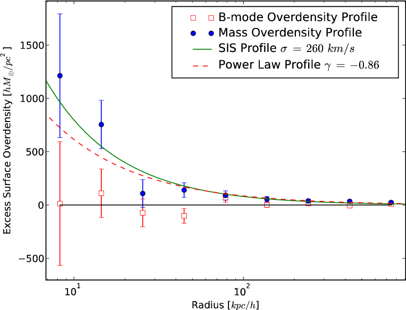
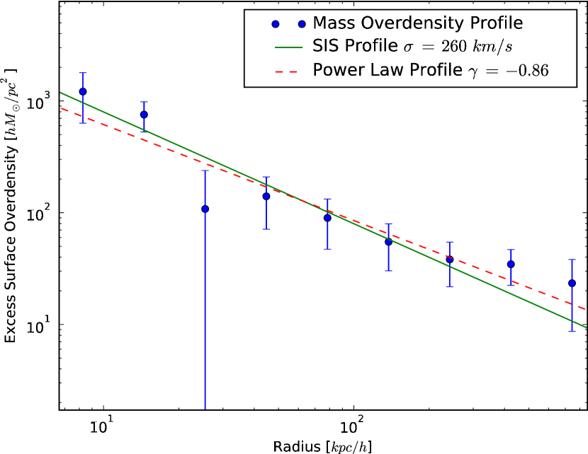
The observed mass overdensity profile can be seen in Figure 2. We can see a significant signal in the (E-mode) profile, while the (B-mode) profile is consistent with zero. Measured values of both and are reported in Table 4, along with their associated shear values. To measure the slope of the density profile, we fit both a generic power law model ( Rγ) and an isothermal model ( R-1) to the data (Figure 2). We find that the best-fit power-law model () does not deviate from the best-fit isothermal model, parameterized by a velocity dispersion of km s-1, by more than 1-. Given our uncertainties, both models are consistent with the data, allowing us to conclude that the average mass overdensity profile of our sample is approximately isothermal.
| Galaxy Counts | Outer Bin Boundariesaa with no known were placed at a fiducial redshift z = 0.6. | ||||||
|---|---|---|---|---|---|---|---|
| ( kpc) | |||||||
| 4 | 11 | 1213 | 13 | 580 | 0.231 | -0.010 | 0.101 |
| 23 | 19 | 755 | 110 | 228 | 0.124 | 0.023 | 0.049 |
| 73 | 33 | 108 | -73 | 130 | 0.024 | -0.010 | 0.027 |
| 233 | 57 | 140 | -102 | 69 | 0.029 | -0.020 | 0.015 |
| 656 | 100 | 90 | 66 | 43 | 0.017 | 0.014 | 0.009 |
| 1851 | 176 | 56 | 2 | 25 | 0.012 | 0.000 | 0.005 |
| 4380 | 308 | 38 | 14 | 16 | 0.007 | 0.004 | 0.004 |
| 8287 | 541 | 33 | -6 | 12 | 0.008 | -0.001 | 0.003 |
| 6997 | 949 | 23 | 8 | 15 | 0.005 | 0.001 | 0.003 |
4.2. Luminous and Dark Matter Profiles
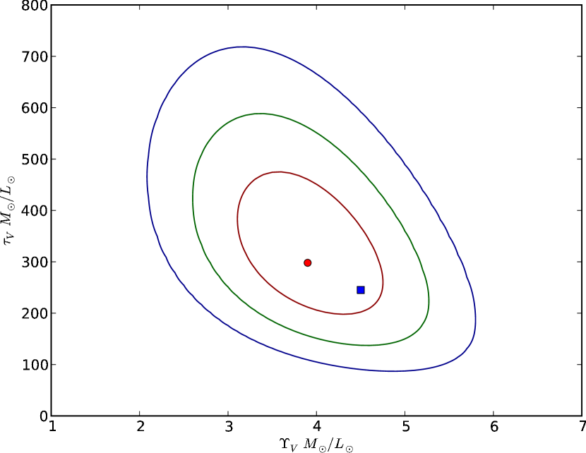
We minimize the total merit function for each of the two approaches: for the mass overdensity fit, and for the reduced shear fit. The best-fit parameters obtained with both approaches can be seen in Figure 3. The results from the model fitting procedures disagree by less than one standard deviation. Thus, we feel we can use the results from the mass overdensity model fit without worrying about inaccuracies in the profile due to the simplifying assumptions made about shear.
The mass overdensity profiles generated from our best-fit parameters are shown in Figure 4, plotted along with the total mass profile from our weak lensing analysis. The figure shows the contributions of the stellar (blue dashed line) and dark matter (red dash-dotted line) mass profiles to the best-fit total mass profile (solid black line). The best fit to our data has , indicating a good agreement between our model and the observed overdensity profile. As a comparison, the pure power-law fit in §4.1 has , meaning that, given our errors, neither the the 1- nor the 2-component model fit is strongly preferred over the other.
We find a virial ratio and a stellar ratio , for an overall virial to stellar mass ratio of . Given the mean V-band luminosity of our sample, , this corresponds to average stellar and virial masses of and respectively. Furthermore, the average virial mass we find corresponds to a typical virial radius of kpc and a typical NFW scale radius of kpc.
Combining our mass ratio data with the assumed cosmology, we are also able to estimate the stellar baryon fraction () present in our lens sample, according to the relation:
| (13) |
where the quantity represents the total baryon to dark matter ratio in the galaxy, and is given by the global value of (Spergel et al., 2007). For our sample, we find a stellar baryon fraction of , which is in excellent agreement with Mandelbaum et al. (2006), who find for their “sm6” bin, consisting of early-type galaxies having and , and in good agreement with Heymans et al. (2006) who find . The Heymans et al. (2006) galaxy sample is somewhat different from our own, in that it consists of both early- and late-type galaxies. The sample is dominated ( ) by early types, though, and the authors note that adopting a more restrictive selection criterion of Sérsic index does not change their results. The average stellar and virial masses of the Heymans et al. (2006) sample ( and , respectively) are an order of magnitude smaller than our own sample, making it difficult to accurately compare results. However, as the Heymans et al. (2006) sample has similar masses to the Mandelbaum et al. (2006) “sm4” early-type sample, scaling this value by gives a result of , which is still within of our value.
Finally, our value is in marginal agreement with Fukugita et al. (1998), who estimate a universal stellar baryon fraction of for spheroids, using data acquired from the local universe.
5. Discussion
5.1. Mass Profiles
Figure 2 shows that the best-fit power law profile to the total mass overdensity data between physical scales of 10 and 1000 kpc has , where . This is consistent with an isothermal () profile and, thus, is similar to the results of G07, who found that the low-redshift SLACS lens sample also displays a characteristically isothermal mass profile between 1 and 300 kpc. However, a closer inspection of the right panel of Figure 2 reveals that we may be seeing some flattening in the profile at large radii. These points are located at distances outside of the average virial radius of our lens sample. Background galaxies located at these radii could thus be affected by the dark matter halos of other massive galaxies nearby the lens, which would explain the larger-than-expected shear signal in the profile. Alternatively, since many of the galaxies in these bins lie near the edge of the ACS field, we could be seeing excess “shear” due to CCD edge effects. Rerunning the profile analysis after excluding the outermost two data bins, we find a best-fit profile that is much more consistent with an isothermal distribution.
Even with the possibility of flattening at large radii, though, combining the results of G07 with our results suggests that the average mass overdensity profile of strong gravitational lenses is consistent with an isothermal model over three orders of magnitude in physical radius. This result is in good agreement with previous mass profile studies of non-lensing ellipticals (Sheldon et al., 2004; Mandelbaum et al., 2006) between kpc, which would suggest that there is little difference between the mass profiles of field strong lenses and their non-lensing counterparts at moderate radii.
| Sample | z | |||
|---|---|---|---|---|
| () | ||||
| SLACS | 0.23 | 5.8 | 54 | 28 |
| z1 | 0.42 | 4.2 | 85 | 33 |
| z2 | 0.83 | 4.8 | 80 | 46 |
Comparing the mean velocity dispersion of our lens sample ( = 260 20 km s-1) to that of the G07 SLACS sample ( 248 km s-1), and noting the broad similarities between the slopes of their mass profiles, it would appear that there is little difference between the overall mass properties of strong lenses at and the properties of those at , although large uncertainties on both profiles could easily hide any real evolutionary results. Additionally, the best-fit ratios of our sample (, ) are not significantly different from those of G07 (, ).
Considering the hierarchical merging model of galaxy formation, which posits that the majority of the mass assembly of massive red ellipticals (the dominant morphology of lensing galaxies) takes place at redshifts 2, it is not surprising that the differences in total mass between these two samples is not dramatic. More surprising however is the fact that the individual ratios do not change, as passive luminosity evolution could significantly affect the total brightness of a galaxy over this redshift range. We investigate the effects of purely passive evolution on the stellar component in two ways, back-evolving the G07 result from to using both the methods of Treu et al. (2001) (method 1) and van Dokkum & Franx (2001) (method 2). After applying these relations, we find a theoretical ratio of using method 1 and using method 2. Both results agree with our measured within the errors. From this, we conclude that the passive evolution and no-evolution models are both plausible descriptions of stellar ratio evolution between and , given the current size of our errors. Future studies with larger sample sizes should be able to place tighter constraints on these parameters, making it easier to distinguish between the possible outcomes.
5.2. Mass Ratio Evolution
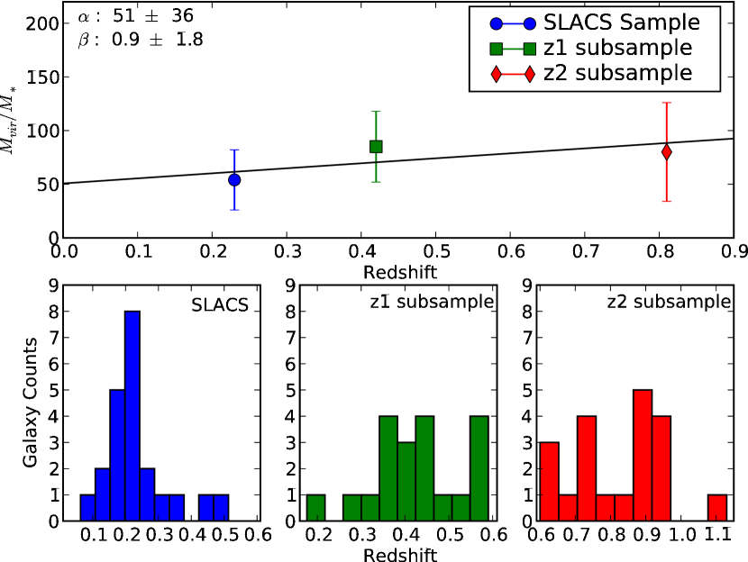
We also search for evidence of the evolution of mass ratio, looking for any significant changes in the ratio of , which could suggest evidence of a merger or satellite accretion event (Conroy et al., 2007). We do this by comparing our results to those of G07, after splitting our sample into two redshift bins: subsample z1, where and subsample z2, where . We fit a slope to the data of the functional form:
| (14) |
The results of the fit can be seen in Figure 5, and the data are presented in Table 5. We find a best-fit and a best-fit , which is consistent with a no-evolution model (). This result is in agreement with the work of Heymans et al. (2006), who use weak-lensing alone to probe the evolution of a sample of predominantly ( 75%) early-type galaxies between and . After explicitly assuming a linear growth factor, they find that = . In using weak-lensing alone however, Heymans et al. (2006) are unable to constrain stellar mass directly, since weak-lensing is not able to probe mass at small radii where stellar matter dominates. Instead, they make an assumption about the nature of stellar mass, using a Kroupa stellar IMF (Kroupa et al., 1993) to scale the average halo mass for their galaxy sample. This is similar to techniques used by other weak-lensing only mass ratio studies, such as Mandelbaum et al. (2006) who used a Kroupa IMF and Hoekstra et al. (2005) who used a scaled Salpeter IMF (Salpeter, 1955).
Unlike these previous studies, our stellar mass values are obtained purely from a luminosity-scaled fit to the mass data, without the need to invoke a specific stellar IMF. Indeed, this is the first such study to attempt to quantify the evolution of the stellar mass ratio without making any assumptions about the nature of the stellar IMF, and the fact that we are able to obtain a consistent result, even with such a small sample of lenses is promising. It is likely that future studies with larger lens samples will be able to place even better constraints on stellar mass evolution, without having to worry about possible systematic errors associated with the IMF, focusing instead on only the lensing-inferred mass and total luminosity, which are both directly determined from the data.
5.3. Mass to Light Ratio Systematics
In determining the best-fit stellar and virial ratios for our lens sample, we determine statistical uncertainties from the model-fitting procedure that are on the order of . In this section, we investigate the impact of systematic uncertainties. Specifically, we look at two such effects: varying the inner slope of the dark matter profile, and modifying the dark matter concentration-mass relation (CMR).

5.3.1 Dark Matter Inner Slope
When discussing the disentanglement of stellar and dark matter, we have, to this point, specifically assumed a standard NFW profile for the dark matter. This has been done not only to take advantage of the analytic form of the dark matter shear profile described in Wright & Brainerd (2000), but also to compare our results to the numerous previous studies that have assumed NFW dark matter profiles as well (e.g. Hoekstra et al. 2005; Mandelbaum et al. 2006; Heymans et al. 2006; G07). Recently however, studies have shown that lensing data actually favor a dark matter profile with a slightly modified inner slope (), often motivated by some physical process such as adiabatic contraction (AC; Blumenthal et al., 1986; Gnedin et al., 2004) that affects the regions of a galaxy where (Jiang & Kochanek, 2007; Gao et al., 2008; Schulz et al., 2009). Because this modification only alters the distribution of the dark matter on small ( kpc) scales for galaxy-scale masses, the total dark matter mass and virial ratio derived from these new profiles remain statistically consistent with the original NFW model. However, this is not the case for the derived stellar ratio (), as even a change in on the order of a few percent can significantly impact , and hence the inferred stellar mass.
To gauge the systematic impact of altering on our data, we rerun the two-component stellar+dark matter analysis described in §3, replacing the standard NFW profile with a generalized NFW (gNFW) profile (e.g. Keeton, 2001):
| (15) |
that is similarly projected into 2-dimensions (see Keeton 2001 for details). While this prescription is somewhat different than applying an AC model to a galaxy (AC also modifies the concentration parameter, whereas altering the gNFW slope does not), the effect on the halo’s inner slope can be comparable: Gnedin et al. (2004) have demonstrated that, assuming an initial NFW dark matter halo with a distribution of baryons that condenses to form an elliptical galaxy, the final inner slope of the dark matter halo ranges between and .
To be conservative, we vary between 0.1 and 1.5, measuring the best-fit V-band stellar ratio () for each case. The results can be seen in Figure 6. We find that the best-fit is strongly dependent on , suggesting a degeneracy between these two parameters that affects stellar mass in the expected way: an increase in dark matter fraction in the core of the galaxy (characterized by a steeper inner slope) results in a smaller fraction of stellar mass (characterized by a lower stellar ratio).
Assuming a fiducial uncertainty on of 20%, the variation in corresponds to a range in stellar ratio of . Adding this systematic uncertainty to our previous estimate of statistical error yields (). As a comparison, Jiang & Kochanek (2007) measure a 30% decrease in stellar ratio by including the Blumenthal et al. (1986) AC model on a subsample of lower-redshift strong lenses, in good agreement with the results we see when we increase the inner slope of the NFW profile by 20%.
5.3.2 Concentration-Mass Relation
By using a CMR to reduce the number of free parameters in our model fitting routine, we are explicitly coupling the best-fit mass to the observed shape of the mass density profile. If instead we were to make different assumptions about the CMR, this would lead to different best-fit mass values, which ultimately would yield systematically different stellar and virial ratios. While we, like G07, have assumed the Bullock et al. (2001) CMR (Equation (5)) in our analysis, recent work involving higher resolution numerical simulations (Macciò et al., 2007, 2008) have argued for an alternative CMR that is less sensitive to halo mass and evolves more slowly with redshift. In particular, using the cosmological parameters from the WMAP 5-year data set, Macciò et al. (2008) determine a CMR of the form:
| (16) |
where is the Hubble parameter. Comparing these CMRs for galaxies with total mass of the order of our sample (), we find that the Macciò et al. (2008) CMR yields a concentration parameter that is smaller than the Bullock et al. (2001) CMR at redshift , but (because of the slower evolution with redshift) actually becomes larger than the Bullock et al. (2001) CMR at , the median redshift of our sample. Re-running our initial de Vaucouleurs + NFW model fit with this new CMR, we find that the best fit and parameters vary by approximately 10% and 5% respectively, which is much less than the statistical uncertainties presented in §4.
In addition to completely modifying the CMR, we also investigate systematics associated with the intrinsic scatter of the relation itself. Including the 1- errors, Bullock et al. (2001) measure a variation in halo concentrations for their sample of halos, which we incorporate into our analysis. Specifically, assuming an extreme case where we increase the concentration parameter of each galaxy in our sample by (and the alternative case where we decrease each halo by ), we measure variations in and of 25% and 15% respectively. Adding these uncertainties in quadrature with the uncertainties associated with our choice of CMR, we therefore include an additional and uncertainty on our best-fit stellar and virial ratios due to the systematics of the CMR.
5.3.3 Propagation of Systematic Uncertainties
Ultimately, by investigating modifications to both the inner slope and concentration parameter of the dark matter halo, we believe that we are able to characterize the potential impact of important systematics on our results, enabling us to propagate these uncertainties to all other measured quantities that depend on them. In particular, we find a total systematic uncertainty of on our best-fit (dominated by the systematics of the dark matter inner slope) and a uncertainty on our best-fit , which subsequently correspond to and uncertainties on our derived stellar and virial masses. Propagating these uncertainties to the other derived parameters, we measure a systematic uncertainty on both the mass ratio (), and stellar baryon fraction .

6. Conclusions and Future Work
Taking advantage of the large density of background galaxies obtained by relatively short ( sec) ACS exposures, we present the results of a joint weak and strong lensing analysis of a sample of 41 massive elliptical galaxies at moderate () redshift, determining the mass overdensity profile over nearly 3 orders of magnitude in physical radius. Using a 2-component de Vaucouleurs + NFW profile model, we are able to determine stellar and virial ratios for the sample, and disentangle the relative contributions of stellar and dark matter from the total mass budget. Furthermore, we compare all of our results to those obtained from a subset of the lower redshift SLACS sample (), placing constraints on the evolution of these mass properties over cosmic time. Our results can be summarized as follows:
-
•
We present new redshift information for 7 COSMOS lenses: we find lens redshifts for J095930.93+023427.7, 0038+4133, J100140.12+020040.9, 0211+1139, and 0216+2955, a source redshift for 0056+1226, and both lens and source redshifts for 0254+1430.
-
•
The mass overdensity profile of our sample has a best-fit power-law profile of and is consistent with an isothermal model between 10 kpc and 1000 kpc.
-
•
The best-fit stellar and virial ratios for our lens sample are given by and respectively.
-
•
Given our average sample luminosity of , we find an average virial mass of and an average stellar mass of .
-
•
We find an average mass ratio of , which is consistent with the lower-redshift SLACS sample ratio of .
- •
-
•
By comparing our mass fraction data to the lower-redshift SLACS sample, we are able to place constraints on the evolution of the virial to stellar mass fraction of massive early-type galaxies. We find that the quantity evolves as / = over the last 7 Gigayears. This is the first such study to place constraints on the evolution of / without invoking a specific IMF.
Overall, these results show that our method is a promising new technique: with only a small sample of lenses (41 systems), were are able to significantly measure the average mass overdensity profile and mass-to-light ratios of the sample, allowing us to place constraints on the mass evolution of early-type galaxies from to . As always though, this work can be strengthened by increasing the sample size. While galaxy-scale strong lenses are relatively rare today ( 100 systems), future large-scale observational surveys such as LSST ( 10000 new lenses) and JDEM ( 10000 new lenses; Marshall et al., 2005) are expected to dramatically increase the number of known strong lenses. Including these new lenses in future work will greatly reduce the size of our present statistical uncertainties.
In the near future however, we plan to increase our lens sample by including other known deep space-based lens data from CASTLES that have been imaged using the smaller HST Wide Field / Planetary Camera 2 (WFPC2). Though the smaller area will limit our ability to probe out to the large radii made available with the ACS sample, the longer exposure times for the WFPC2 data yield background densities that are comparable to those in the ACS sample, allowing us to place better constraints on the inner mass overdensity profile by incorporating these galaxies into our current lens sample. We will also take advantage of the HAGGLeS strong-lens search of bright red galaxies (Marshall et al., 2009) which is expected to explore the whole of the HST ACS archive, discovering 10 lenses per square degree of coverage. We plan to further augment this study by combining our ACS sample with the full ( 40) long-exposure SLACS sample, which will allow us to probe the differences in the mass properties of strong lenses across a wider variety of samples and categories, such as morphology, luminosity, and finer redshift slices. We are particularly interested in segregating the lens sample by total luminosity, since the SLACS lenses appear to be more luminous than their moderate-redshift counterparts when passively evolved to (Figure 7), suggesting that the SLACS sample may have evolved from a slightly different population of galaxies.
Of course, by increasing the sample size of lenses and thus reducing the statistical errors associated with these measurements, correcting systematic uncertainties will become much more important. In future studies we hope to improve our control of systematics in several ways. Foremost is the ability to measure accurate redshifts for both the lens and source galaxies of strong lens systems, as these measurements are crucial for accurate lens modeling. While some future survey instruments should provide redshift information (either spectroscopically or photometrically) as part of their normal operation, it is still important to improve the redshift information for currently known lenses, and we plan to obtain more spectroscopic and photometric redshift data in the near future. Additional systematics controls could come in the form of improved profile modeling, relaxing the strict de Vaucoulers + NFW mass profiles in favor of a more general free-index Sérsic profile for the stellar mass and a freely-varying gNFW profile for the dark matter. Similarly, improved strong lens mass modeling should be utilized in the future, increasing our ability to distinguish between various mass profiles at very small scales, as well as improving the precision of our stellar mass fraction measurements. Finally, we could improve galaxy selection and weak lensing measurements by using HST data obtained through other filters, allowing us to determine photometric redshifts for many of the background source galaxies. We note however that this should not be a dominant source of systematic error, as we have shown previously that altering the background galaxy redshift distribution does not significantly change the results of any of our fitted parameters.
References
- Andersen et al. (2006) Andersen, D. R., Bershady, M. A., Sparke, L. S., Gallagher, J. S., III, Wilcots, E. M., van Driel, W., & Monnier-Ragaigne, D. 2006, ApJS, 166, 505
- Anguita et al. (2009) Anguita, T., Faure, C., Kneib, J.-P., Wambsganss, J., Knobel, C., Koekemoer, A. M., & Limousin, M. 2009, A&A, 507, 35
- Argo et al. (2003) Argo, M. K., et al. 2003, MNRAS, 338, 957
- Arnaboldi et al. (2004) Arnaboldi, M., Gerhard, O., Aguerri, J. A. L., Freeman, K. C., Napolitano, N. R., Okamura, S., & Yasuda, N. 2004, ApJ, 614, L33
- Avila-Reese et al. (2008) Avila-Reese, V., Zavala, J., Firmani, C., & Hernández-Toledo, H. M. 2008, AJ, 136, 1340
- Bartelmann & Schneider (2001) Bartelmann, M., & Schneider, P. 2001, Phys. Rep., 340, 291
- Bertin et al. (1994) Bertin, G., et al. 1994, A&A, 292, 381
- Bertin & Arnouts (1996) Bertin, E., & Arnouts, S. 1996, A&AS, 117, 393
- Biggs et al. (2003) Biggs, A. D., et al. 2003, MNRAS, 338, 1084
- Blackburne et al. (2008) Blackburne, J. A., Wisotzki, L., & Schechter, P. L. 2008, AJ, 135, 374
- Blumenthal et al. (1984) Blumenthal, G. R., Faber, S. M., Primack, J. R., & Rees, M. J. 1984, Nature, 311, 517
- Blumenthal et al. (1986) Blumenthal, G. R., Faber, S. M., Flores, R., & Primack, J. R. 1986, ApJ, 301, 27
- Bolton et al. (2006) Bolton, A. S., Burles, S., Koopmans, L. V. E., Treu, T., & Moustakas, L. A. 2006, ApJ, 638, 703
- Bolton et al. (2008) Bolton, A. S., Treu, T., Koopmans, L. V. E., Gavazzi, R., Moustakas, L. A., Burles, S., Schlegel, D. J., & Wayth, R. 2008, ApJ, 684, 248
- Brainerd et al. (1996) Brainerd, T. G., Blandford, R. D., & Smail, I. 1996, ApJ, 466, 623
- Browne et al. (1993) Browne, I. W. A., Patnaik, A. R., Walsh, D., & Wilkinson, P. N. 1993, MNRAS, 263, L32
- Bryan & Norman (1998) Bryan, G. L., & Norman, M. L. 1998, ApJ, 495, 80
- Bullock et al. (2001) Bullock, J. S., Kolatt, T. S., Sigad, Y., Somerville, R. S., Kravtsov, A. V., Klypin, A. A., Primack, J. R., & Dekel, A. 2001, MNRAS, 321, 559
- Cappellari et al. (2006) Cappellari, M., et al. 2006, MNRAS, 366, 1126
- Churazov et al. (2008) Churazov, E., Forman, W., Vikhlinin, A., Tremaine, S., Gerhard, O., & Jones, C. 2008, MNRAS, 388, 1062
- Conroy et al. (2007) Conroy, C., Wechsler, R. H., & Kravtsov, A. V. 2007, ApJ, 668, 826
- Crampton et al. (2002) Crampton, D., Schade, D., Hammer, F., Matzkin, A., Lilly, S. J., & Le Fèvre, O. 2002, ApJ, 570, 86
- de Lorenzi et al. (2008) de Lorenzi, F., Gerhard, O., Saglia, R. P., Sambhus, N., Debattista, V. P., Pannella, M., & Méndez, R. H. 2008, MNRAS, 385, 1729
- de Vaucouleurs (1948) de Vaucouleurs, G. 1948, Annales d’Astrophysique, 11, 247
- Diemand et al. (2007) Diemand, J., Kuhlen, M., & Madau, P. 2007, ApJ, 657, 262
- Eigenbrod et al. (2006, a) Eigenbrod, A., Courbin, F., Dye, S., Meylan, G., Sluse, D., Vuissoz, C., & Magain, P. 2006, A&A, 451, 747
- Eigenbrod et al. (2006, b) Eigenbrod, A., Courbin, F., Meylan, G., Vuissoz, C., & Magain, P. 2006, A&A, 451, 759
- Eke et al. (2001) Eke, V. R., Navarro, J. F., & Steinmetz, M. 2001, ApJ, 554, 114
- Erben et al. (2001) Erben, T., Van Waerbeke, L., Bertin, E., Mellier, Y., & Schneider, P. 2001, A&A, 366, 717
- Fassnacht et al. (1996) Fassnacht, C. D., Womble, D. S., Neugebauer, G., Browne, I. W. A., Readhead, A. C. S., Matthews, K., & Pearson, T. J. 1996, ApJ, 460, L103
- Faure et al. (2008) Faure, C., et al. 2008, ApJS, 176, 19
- Fischer et al. (2000) Fischer, P., et al. 2000, AJ, 120, 1198
- Ford et al. (1998) Ford, H. C., et al. 1998, Proc. SPIE, 3356, 234
- Fukugita et al. (1998) Fukugita, M., Hogan, C. J., & Peebles, P. J. E. 1998, ApJ, 503, 518
- Gao et al. (2008) Gao, L., Navarro, J. F., Cole, S., Frenk, C. S., White, S. D. M., Springel, V., Jenkins, A., & Neto, A. F. 2008, MNRAS, 387, 536
- Gavazzi & Soucail (2007) Gavazzi, R., & Soucail, G. 2007, A&A, 462, 459
- Gavazzi et al. (2007) Gavazzi, R., Treu, T., Rhodes, J. D., Koopmans, L. V. E., Bolton, A. S., Burles, S., Massey, R. J., & Moustakas, L. A. 2007, ApJ, 667, 176
- Gentile et al. (2004) Gentile, G., Salucci, P., Klein, U., Vergani, D., & Kalberla, P. 2004, MNRAS, 351, 903
- Gentile et al. (2007) Gentile, G., Tonini, C., & Salucci, P. 2007, A&A, 467, 925
- Gnedin et al. (2004) Gnedin, O. Y., Kravtsov, A. V., Klypin, A. A., & Nagai, D. 2004, ApJ, 616, 16
- Grillo et al. (2009) Grillo, C., Gobat, R., Lombardi, M., & Rosati, P. 2009, A&A, 501, 461
- Heymans et al. (2006) Heymans, C., et al. 2006, MNRAS, 371, L60
- Hoekstra et al. (1998) Hoekstra, H., Franx, M., Kuijken, K., & Squires, G. 1998, ApJ, 504, 636
- Hoekstra et al. (2005) Hoekstra, H., Hsieh, B. C., Yee, H. K. C., Lin, H., & Gladders, M. D. 2005, ApJ, 635, 73
- Humphrey et al. (2006) Humphrey, P. J., Buote, D. A., Gastaldello, F., Zappacosta, L., Bullock, J. S., Brighenti, F., & Mathews, W. G. 2006, ApJ, 646, 899
- Ilbert et al. (2009) Ilbert, O., et al. 2009, ApJ, 690, 1236
- Inada et al. (2003) Inada, N., et al. 2003, AJ, 126, 666
- Inada et al. (2005) Inada, N., et al. 2005, AJ, 130, 1967
- Inada et al. (2008) Inada, N., et al. 2008, AJ, 135, 496
- Jackson (2008) Jackson, N. 2008, MNRAS, 389, 1311
- Jackson et al. (2004) Jackson, D. C., Skillman, E. D., Cannon, J. M., & Côté, S. 2004, AJ, 128, 1219
- Jiang & Kochanek (2007) Jiang, G., & Kochanek, C. S. 2007, ApJ, 671, 1568
- Jing (2000) Jing, Y. P. 2000, ApJ, 535, 30
- Johnston et al. (2003) Johnston, D. E., et al. 2003, AJ, 126, 2281
- Kaiser et al. (1995) Kaiser, N., Squires, G., & Broadhurst, T. 1995, ApJ, 449, 460
- Keeton (2001) Keeton, C. R. 2001, arXiv:astro-ph/0102341
- Kinney et al. (1996) Kinney, A. L., Calzetti, D., Bohlin, R. C., McQuade, K., Storchi-Bergmann, T., & Schmitt, H. R. 1996, ApJ, 467, 38
- Kleinheinrich et al. (2006) Kleinheinrich, M., et al. 2006, A&A, 455, 441
- Koekemoer et al. (2002) Koekemoer, A. M., Fruchter, A. S., Hook, R. N., & Hack, W. 2002, The 2002 HST Calibration Workshop : Hubble after the Installation of the ACS and the NICMOS Cooling System, Proceedings of a Workshop held at the Space Telescope Science Institute, Baltimore, Maryland, October 17 and 18, 2002. Edited by Santiago Arribas, Anton Koekemoer, and Brad Whitmore. Baltimore, MD: Space Telescope Science Institute, 2002., p.337, 337
- Krist (2003) Krist, J. 2003, Instrument Science Rep. ACS 2003-06 (Baltimore: STScI), http://www.stsci.edu/hst/acs/documents/isrs/isr0306.pdf
- Kroupa et al. (1993) Kroupa, P., Tout, C. A., & Gilmore, G. 1993, MNRAS, 262, 545
- Kuhlen et al. (2008) Kuhlen, M., Diemand, J., Madau, P., & Zemp, M. 2008, Journal of Physics Conference Series, 125, 012008
- Kuzio de Naray et al. (2008) Kuzio de Naray, R., McGaugh, S. S., & de Blok, W. J. G. 2008, ApJ, 676, 920
- Lacy et al. (2002) Lacy, M., Gregg, M., Becker, R. H., White, R. L., Glikman, E., Helfand, D., & Winn, J. N. 2002, AJ, 123, 2925
- Lawrence (1996) Lawrence, C. R. 1996, Astrophysical Applications of Gravitational Lensing, 173, 299
- Lehár et al. (2001) Lehár, J., Buchalter, A., McMahon, R. G., Kochanek, C. S., & Muxlow, T. W. B. 2001, ApJ, 547, 60
- Macciò et al. (2007) Macciò, A. V., Dutton, A. A., van den Bosch, F. C., Moore, B., Potter, D., & Stadel, J. 2007, MNRAS, 378, 55
- Macciò et al. (2008) Macciò, A. V., Dutton, A. A., & van den Bosch, F. C. 2008, MNRAS, 391, 1940
- Mandelbaum et al. (2006) Mandelbaum, R., Seljak, U., Kauffmann, G., Hirata, C. M., & Brinkmann, J. 2006, MNRAS, 368, 715
- Marshall et al. (2005) Marshall, P., Blandford, R., & Sako, M. 2005, New Astronomy Review, 49, 387
- Marshall et al. (2009) Marshall, P. J., Hogg, D. W., Moustakas, L. A., Fassnacht, C. D., Bradač, M., Schrabback, T., & Blandford, R. D. 2009, ApJ, 694, 924
- Matthews & Uson (2008) Matthews, L. D., & Uson, J. M. 2008, AJ, 135, 291
- Merrett et al. (2006) Merrett, H. R., et al. 2006, MNRAS, 369, 120
- Monet et al. (2003) Monet, D. G., et al. 2003, AJ, 125, 984
- Moore et al. (1998) Moore, B., Governato, F., Quinn, T., Stadel, J., & Lake, G. 1998, ApJ, 499, L5
- Morgan et al. (2004) Morgan, N. D., Caldwell, J. A. R., Schechter, P. L., Dressler, A., Egami, E., & Rix, H.-W. 2004, AJ, 127, 2617
- Morgan et al. (2005) Morgan, N. D., Kochanek, C. S., Pevunova, O., & Schechter, P. L. 2005, AJ, 129, 2531
- Moustakas et al. (2007) Moustakas, L. A., et al. 2007, ApJ, 660, L31
- Myers et al. (1995) Myers, S. T., et al. 1995, ApJ, 447, L5
- Napolitano et al. (2009) Napolitano, N. R., et al. 2009, MNRAS, 393, 329
- Navarro et al. (1997) Navarro, J. F., Frenk, C. S., & White, S. D. M. 1997, ApJ, 490, 493
- Oke et al. (1995) Oke, J. B., et al. 1995, PASP, 107, 375
- Parker et al. (2007) Parker, L. C., Hoekstra, H., Hudson, M. J., van Waerbeke, L., & Mellier, Y. 2007, ApJ, 669, 21
- Patnaik et al. (1993) Patnaik, A. R., Browne, I. W. A., King, L. J., Muxlow, T. W. B., Walsh, D., & Wilkinson, P. N. 1993, MNRAS, 261, 435
- Peng et al. (2002) Peng, C. Y., Ho, L. C., Impey, C. D., & Rix, H.-W. 2002, AJ, 124, 266
- Peterson et al. (1978) Peterson, C. J., Rubin, V. C., Ford, W. K., Jr., & Roberts, M. S. 1978, ApJ, 226, 770
- Pindor et al. (2004) Pindor, B., et al. 2004, AJ, 127, 1318
- Rhodes et al. (2007) Rhodes, J. D., et al. 2007, ApJS, 172, 203
- Romanowsky et al. (2003) Romanowsky, A. J., Douglas, N. G., Arnaboldi, M., Kuijken, K., Merrifield, M. R., Napolitano, N. R., Capaccioli, M., & Freeman, K. C. 2003, Science, 301, 1696
- Rubin et al. (1979) Rubin, V. C., Ford, W. K. J., & Roberts, M. S. 1979, ApJ, 230, 35
- Salpeter (1955) Salpeter, E. E. 1955, ApJ, 121, 161
- Salucci (2001) Salucci, P. 2001, MNRAS, 320, L1
- Sand et al. (2008) Sand, D. J., Treu, T., Ellis, R. S., Smith, G. P., & Kneib, J.-P. 2008, ApJ, 674, 711
- Schlegel et al. (1998) Schlegel, D. J., Finkbeiner, D. P., & Davis, M. 1998, ApJ, 500, 525
- Schmidt et al. (2008) Schmidt, K. B., Hansen, S. H., & Macciò, A. V. 2008, ApJ, 689, L33
- Schrabback et al. (2007) Schrabback, T., et al. 2007, A&A, 468, 823
- Schulz et al. (2009) Schulz, A. E., Mandelbaum, R., & Padmanabhan, N. 2009, arXiv:0911.2260
- Seigar et al. (2008) Seigar, M. S., Barth, A. J., & Bullock, J. S. 2008, MNRAS, 389, 1911
- Seitz & Schneider (1997) Seitz, C., & Schneider, P. 1997, A&A, 318, 687
- Sheldon et al. (2004) Sheldon, E. S., et al. 2004, AJ, 127, 2544
- Simon et al. (2005) Simon, J. D., Bolatto, A. D., Leroy, A., Blitz, L., & Gates, E. L. 2005, ApJ, 621, 757
- Sluse et al. (2003) Sluse, D., et al. 2003, A&A, 406, L43
- Spergel et al. (2007) Spergel, D. N., et al. 2007, ApJS, 170, 377
- Stoehr (2006) Stoehr, F. 2006, MNRAS, 365, 147
- Treu et al. (2001) Treu, T., Stiavelli, M., Bertin, G., Casertano, S., & Møller, P. 2001, MNRAS, 326, 237
- Treu et al. (2006) Treu, T., Koopmans, L. V., Bolton, A. S., Burles, S., & Moustakas, L. A. 2006, ApJ, 640, 662
- Uson & Matthews (2003) Uson, J. M., & Matthews, L. D. 2003, AJ, 125, 2455
- van der Wel & van der Marel (2008) van der Wel, A., & van der Marel, R. P. 2008, ApJ, 684, 260
- van Dokkum & Franx (2001) van Dokkum, P. G., & Franx, M. 2001, ApJ, 553, 90
- White & Rees (1978) White, S. D. M., & Rees, M. J. 1978, MNRAS, 183, 341
- Wilson et al. (2001) Wilson, G., Kaiser, N., Luppino, G. A., & Cowie, L. L. 2001, ApJ, 555, 572
- Wisotzki et al. (2002) Wisotzki, L., Schechter, P. L., Bradt, H. V., Heinmüller, J., & Reimers, D. 2002, A&A, 395, 17
- Wittman (2002) Wittman, D. 2002, Gravitational Lensing: An Astrophysical Tool, 608, 55
- Wright & Brainerd (2000) Wright, C. O., & Brainerd, T. G. 2000, ApJ, 534, 34
- York et al. (2005) York, T., et al. 2005, MNRAS, 361, 259
Appendix A Weak Lensing Analysis
A.1. Object Detection and Shape Measurement
This study utilizes the IMCAT888http://www.ifa.hawaii.edu/kaiser/imcat/ software suite, which is based on the well-known algorithm of Kaiser, Squires, & Broadhurst (1995, hereafter KSB), as well as a series of Perl and Python scripts which apply the PSF correction scheme of Schrabback et al. (2007) and mass profile analysis of G07. Using both the catalogs and their associated science images, our pipeline first invokes the IMCAT object detection program hfindpeaks on the images and cross-correlates the results with the related SExtractor catalogs, in order to reduce the number of false detections. Objects detected in both SExtractor and hfindpeaks are convolved with a Gaussian smoothing kernel in order to regularize their shapes and sizes and also to reduce shape noise; the width of an object’s smoothing kernel () is given by the object’s half light radius as determined by SExtractor. Once an object has been smoothed, the local sky background is calculated and subtracted from its overall intensity. After background subtraction, the object’s magnitude is determined using a magnitude zero point taken from the ACS website999http://www.stsci.edu/hst/acs/.
Finally, the script determines a centroid for each object, and calculates the quadrupole moments of intensity, given by
| (A1) |
where the integral is taken from the centroid location to . Here, represents the intensity of an object in a given pixel, and is a weight function, which for this study is a circular Gaussian with radius , matching the filter used for object detection. These moments of intensity are then used to calculate “ellipticity polarizations”:
| (A2) | |||
| (A3) |
which represent the components of the observed shape of the object. In addition, the “smear” and “shear” polarizability pseudo-tensors ( and respectively; see e.g. KSB, or the updated definitions in Hoekstra et al., 1998) are also calculated, which are used to correct shape measurement errors due to PSF distortion.
A.2. Charge Transfer Inefficiency Correction
Before we analyze the weak lensing signal, we must correct for any systematic distortions of the galaxy shapes. The first such systematic that we address is distortion due to the degradation of charge transfer efficiency (CTE) of the ACS CCDs. Defects that arise during the lifetime of the CCD can cause some charge to be delayed and transferred to other pixels, resulting in a trail of charge following an object. In the ACS, the readout direction is vertical. Thus, this trail will induce a spurious stretching in the direction. Since CTE degradation alters the shapes of galaxies in the same direction, the effect can mimic the gravitational shear signal caused by weak lensing. The spurious polarization induced by CTE degradation is typically on the order of 1%, and therefore it most strongly affects the outer regions of a galaxy-galaxy shear profile (where the gravitational shear drops below 1%). If left uncorrected, this spurious signal can alter the inferred total mass of the galaxy.
The “strength” of an object’s tail is affected by several factors, including object brightness, size, and location along the CCD readout path. This makes for an inherently non-linear problem that cannot be corrected by a simple model. Instead, we use the empirical prescription of Rhodes et al. (2007) devised for the COSMOS program. Following G07, we modify the original equation to be compatible to our data, although we use a slightly different prefactor which accounts for combining the IMCAT definition of SNR with the SExtractor measured half-light radius (G07 obtain both parameters from IMCAT, whereas Rhodes et al. (2007) use SExtractor exclusively):
| (A4) |
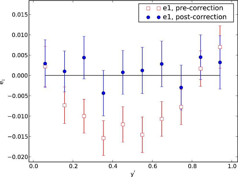
which modifies the component of each object in a catalog. In this equation, represents the half-light radius of the object (as determined by IMCAT), and is the normalized y-coordinate of the object (equal to 0 at the bottom of an ACS field and 1 at the top), defined such that the correction for the CTE degradation is maximized near the ACS chip gap (), where the pixels are the farthest away from the readout registers. The time-dependent factor takes into account the fact that the effects of CTE degradation have steadily worsened over the lifetime of the ACS.
Figure 8 shows the effect of CTE correction on our data sample, and from the figure we can see that the average corrected galaxy shape () is no longer spatially dependent, and is very nearly zero throughout the entire field. In addition, our CTE correction scheme is able to correct specifically chosen subsets of the galaxy population as well: after separating the source galaxies into three distinct magnitude bins (m 25; 25 m 26; m 26), we find that the CTE-corrected galaxies in each bin show a mean shape , again with no spatial dependence across the field.
To test the systematics associated with our CTE correction scheme, we apply an additional 20% CTE shape correction to every background galaxy, regardless of size, brightness, or position on the detector. We perform a full weak lensing analysis and 2-component model-fit (§3) on these data, and find that the best-fit stellar and virial ratios systematically vary from the values inferred from the original data (presented in §4) by and respectively, which are much smaller than the presented statistical errors.
A.3. PSF Correction
We next perform a PSF correction to remove any shape distortions of the background galaxies due to the telescope, leaving only those distortions caused by gravitational shear. Our correction scheme applies the method of Schrabback et al. (2007), which utilizes the KSB formalism along with modifications developed by Hoekstra et al. (1998) and Erben et al. (2001).
While it should be possible to map the spatial variations of the PSF by directly measuring the shapes of the stars found in the data, we find that this is not the case for our lens sample, as there are too few stars per exposure to accurately sample the whole field. Instead, to increase our star count we use a series of well-sampled, low galactic latitude stellar field exposures to generate a series of polynomial PSF models. There is some concern in fitting a model PSF to our data instead of deriving it empirically, as the ACS PSF is temporally variable. However, this variability is primarily a function of a single parameter: changes in the separation of the primary and secondary HST mirrors due to thermal breathing (Krist, 2003; Rhodes et al., 2007). By using a total of 181 exposures taken over the course of several months, our stellar-field PSF models span a wide range of mirror separations, allowing us to compile a nearly continuous database of varying PSF patterns that can be used to correct our science images.
To create each model, we measure the anisotropy components () and polarization tensor ratio () – a parameter required for PSF correction that is related to the PSF width – as a function of position, using the stars in a given stellar field. The measured quantities are given by:
| (A5) | ||||
| (A6) |
where are the measured stellar ellipticity components, and and are the stars’ shear and smear polarization tensors, respectively.
Model stars are initially selected by simple cuts in size-magnitude space. A 0.8 pixel wide cut in half-light radius, centered on the stellar locus, is used to separate stars from galaxies. A bright-end magnitude cut is used to remove stars with saturated pixels and a SNR cut is used to remove stars that are too noisy to be accurately measured. From this initial star selection we generate 3rd-order polynomial models for the components, and a 5th-order polynomial model for . To improve the model, we evaluate each polynomial component at the coordinates of the stars, and compare the inferred values to the actual measured quantities. If, for any given model component, the observed value disagrees with the model by more than 2-, the star is considered an outlier (because of shape noise) and is removed from the sample. Once all outliers are removed, we regenerate the polynomial models with the remaining stars. This process is repeated iteratively until the number of stars remains stable, at which point we generate a final set of polynomials that represent the final PSF model for that stellar field.
For each science exposure, we compare the measured PSF of each star in the field to the model PSFs, and determine the best-fit model by calculating the reduced statistic given by:
| (A7) |
where is the measured PSF of star , and is the model PSF of stellar template , evaluated at the location of the real star.
Once best-fit PSF models are determined for all exposures associated with a composite science image, the coordinates of each model are registered to the science image, and the models are combined by an exposure-time weighted average to create a final “master” PSF model used to correct each background galaxy, given by:
| (A8) |
where is the exposure time of a given exposure in the composite science image, and is equal to 1 if the galaxy falls within the boundaries of the WFC chips in the exposure (not always true, due to dithering), and 0 otherwise.
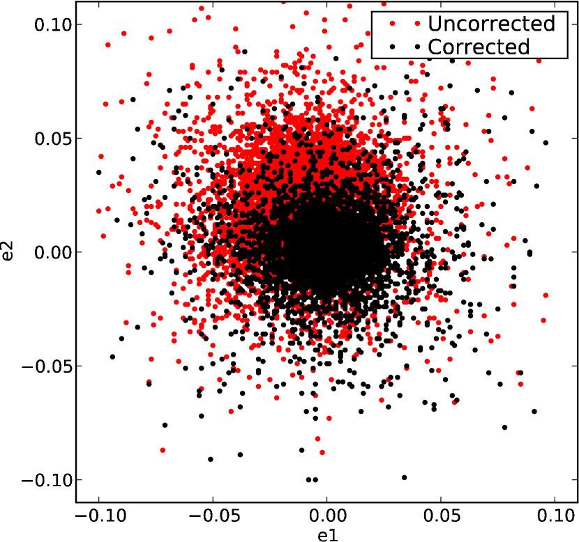
As a test of our PSF correction, we plot the shapes of all stars found in our science images, both pre- and post-correction, (Figure 9). We do see an improvement: the stellar ellipticity components become more circular (, ; , ), and show a mild reduction in spread (, ; ,). By taking into account effects due to the PSF (and effects due to CTE degradation in the previous section) we are able to significantly reduce the dominant sources of systematic error involved in the weak lensing analysis.
A.4. Data Cuts
To improve the overall signal, we apply a series of data cuts to our master catalog. First, we exclude objects that have a half-light radius smaller than 3 pixels, as many of these objects are “bad” data objects such as stars or cosmic rays, which are not affected by gravitational shear and only serve to dilute the overall shear signal. We also reject objects with a half-light radius larger than 14 pixels, and “bright” objects (), as these objects are likely to be foreground interlopers. Additionally, we apply a conservative cut to galaxy shapes, rejecting any object with (where the are the CTE + PSF corrected ellipticity components) as being unphysical or poorly shape-corrected in some way. Finally, we apply a general SNR cut to the data, rejecting any remaining object with an IMCAT significance () parameter less than 16; (as a comparison, this corresponds to an SNR 4 cut using the SNR determination of Erben et al. (2001)). After cutting the data, we are left with a total background galaxy density of galaxies arcmin-2 (as compared to the galaxies arcmin-2 measured prior to cutting) which is high enough to measure the weak lensing signal around the galaxy stack.
A.5. Catalog Stacking
After correcting for PSF and CTE effects for objects in an individual science field, we can apply the standard weak lensing formalism (see e.g., Seitz & Schneider, 1997; Bartelmann & Schneider, 2001; Wittman, 2002) to the field and determine an average mass profile from a stack of fields.
To properly combine each lens field into a cohesive stack, we first apply a shift to the coordinates of each science field, such that the origin in each field corresponds to the location of the strong lens system. Because the lenses in our sample cover a range of redshifts, we convert each background galaxy’s angular separation from the lens to a physical one, so that we can more easily stack galaxy fields together in catalog space. Finally, once all objects have been repositioned in terms of physical distances relative to a common center, we combine everything into a master galaxy catalog that contains information on galaxy position and corrected ellipticity, and information on the strong lens field from which it was initially drawn. In addition, geometric information about the strong lenses themselves are also included, which are critical in determining the physical mass profile at small scales.
A.6. Shear and Mass Profiles
Since our master galaxy catalog contains information on both position and corrected ellipticity, we can combine these parameters to develop two radial shear profiles: a tangential “E-mode” profile given by:
| (A9) |
and a 45 rotated “B-mode” profile, given by:
| (A10) |
where refers to the number of galaxies located within a radial bin centered at radius and and represent the shear components of galaxy , equivalent to the components of reduced shear () in the limit of weak lensing. We calculate and in concentric circular annuli around the common center of our stacked lens sample. For a system with a single lens plane (or a stacked, coincident lens plane) the lensing signal measured with respect to the center of mass and averaged over all background galaxies should be contained entirely within the E-mode profile while the B-mode should vanish. Thus, by computing these two shear profiles, we can see information regarding the radial characteristics of the shear field from , as well as a check on systematic errors from .
Next, we convert shear into a differential surface mass overdensity, , by scaling the tangential shear profile by the critical lensing density :
| (A11) |
a measurement of surface mass density that encodes the angular diameter distances between the observer and the lens (), the observer and the source (), and the lens and the source (). The profile is thus given by:
| (A12) |
where represents the average surface mass density enclosed within projected radius R. Since is a function of both lens and source redshifts ( and , respectively), in principle we must construct a unique for every source galaxy that is used in the mass overdensity profile. In practice, however, this is impractical since a large number of background galaxies do not have measured redshifts. Instead, as in G07, we define an average critical density for each lens field:
| (A13) |
where is a weighted factor of (/), designed to fully account for background source redshift distribution. It is given by:
| (A14) |
where is the redshift distribution of background source galaxies. Since our image exposure times and data cuts are similar to G07 we use their redshift distribution, extrapolated from COSMOS:
| (A15) |
with = 0.345, = 3.89, and = 1. From these parameters, we calculate a mean background source redshift of . A full list of parameters can be seen in Table 1.
We next compute an estimator of :
| (A16) |
where is the number of background galaxies associated with lens field , is the average critical density for lens field , and is the uncertainty assigned to the tangential shear estimate of galaxy , which we take to be the shape uncertainty as defined in Gavazzi & Soucail (2007) to be proportional to a galaxy’s shape measurement error added in quadrature with the intrinsic shape noise of all galaxies () to prevent over-weighting. With this conversion, we are able to transform shear to mass, and develop a mass overdensity profile for our data.
As a check on the systematics of our assumed redshift distribution, we vary the parameters of the distribution, calculating a unique set of {} parameters for each lens field. We do this by measuring the observed F814W magnitude distribution of the galaxies in the field and convert this to a redshift distribution, using the method described in Schrabback et al. (2007). After doing this, we recalculate the , , and estimator values for the entire sample, and repeat the weak lensing analysis with these updated values. We find that, regardless of the choice of redshift distribution parameters, the best-fit model parameters determined here (as well as those described in §3) vary by . Since this is smaller than the statistical uncertainty of our measurements, we conclude that uncertainties in the redshift distribution are negligible for our purposes.