Galaxy Counts on the CMB Cold Spot

Abstract

The Cold Spot on the Cosmic Microwave Background could arise due to a supervoid at low redshift through the integrated Sachs-Wolfe effect. We imaged the region with MegaCam on the Canada-France-Hawai’i Telescope and present galaxy counts in photometric redshift bins. We rule out the existence of a 100Mpc radius spherical supervoid with underdensity $\delta=-0.3$ at $0.5<z<0.9$ at high significance. The data are consistent with an underdensity at low redshift, but the fluctuations are within the range of cosmic variance and the low density areas are not contiguous on the sky. Thus, we find no strong evidence for a supervoid. We cannot resolve voids smaller than 50Mpc radius; however, these can only make a minor contribution to the CMB temperature decrement.

1. Introduction

The nature of the Cold Spot on the Cosmic Microwave Background (CMB) has been the source of broad speculation. The 10° diameter region identified in Wilkinson Microwave Anisotropy Probe (WMAP) temperature maps (Bennett et al., 2003) is curious due to its pronounced temperature and morphology. Extensive study of the region was first motivated by the Spot’s non-Gaussian properties (Vielva et al., 2004; Cruz et al., 2005). Under the standard cosmological model, the primordial fluctuations on the CMB are homogeneous, isotropic and described by a Gaussian random field. In this scenario, the existence of the Spot is unlikely at the $\sim$0.5% level (Cruz et al., 2006), although see Zhang & Huterer (2010) for a critical view. The mean temperature decrement within a 5° radius is $\Delta T=-100$$\mathrm{\mu K}$, and it shows no systematic variation with frequency in WMAP data, making it inconsistent with contamination from synchrotron or dust emission (Cruz et al., 2006; Rudnick et al., 2007).

Many sources of secondary anisotropies have been proposed to explain the Cold Spot, including the integrated Sachs-Wolfe (ISW) and Sunyaev-Zeldovich (SZ) effect, as well as more exotic physics including textures arising in the early Universe. Evidently there is no sufficiently massive cluster in the local universe to produce an SZ temperature decrement over such a large angular scale; however, the other hypotheses have not been directly addressed through observations. Cruz et al. (2008) review these possibilities.

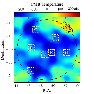
Figure 1.— The 7 Cold Spot fields overlaying the WMAP linear combination (ILC) temperature map. The dashed circle indicates the angular scale of 100Mpc radius at z=0.5.

In this work, we address the question of whether a supervoid exists along the line-of-sight. A significant CMB decrement can be induced by a time-varying gravitational potential through the integrated Sachs-Wolfe effect (ISW) (Sachs & Wolfe, 1967). On linear scales, CMB photons traversing a large-scale void lose energy as the potential decays under the accelerated cosmological expansion. Non-linear structure growth can also contribute to a cold imprint on the CMB through the Rees-Sciama effect (Rees & Sciama, 1968).

This scenario garnered interest due to the recent direct measurement of voids imprinted on the CMB (Granett et al., 2008). The 10$\mathrm{\mu K}$ signal was measured on 4° scales and has been speculated to arise from 100Mpc scale underdensities. Could a similar structure be responsible for the Cold Spot? Furthermore, Rudnick et al. (2007) found a coincidental depression in source counts in the NRAO VLA Sky Survey (NVSS), although the significance of this alignment has been debated (Smith & Huterer, 2010). Through an independent methodology, McEwen et al. (2007) found that the Cold Spot region contributes strongly to the positive NVSS-WMAP cross correlation. These findings motivate further investigation of the void hypothesis.

Survey data covering the Cold Spot are limited. The ISW signal arising from the local Universe has been studied by Maturi et al. (2007) who consider structures within 100Mpc. They find no significant signal at the location of the Cold Spot. Francis & Peacock (2009) investigate the ISW signal traced by 2MASS at $z<0.3$. They detect an underdensity at the Cold Spot, but find that it contributes to the temperature decrement by only 5%.

The Cold Spot is most prominent in a compensated filter. Cruz et al. (2006) use a Spherical Mexican Hat Wavelet with a scale radius of 4.17° and find a temperature decrement of $-16.09$$\mathrm{\mu K}$ in this filter with a 1$\sigma$ range due to cosmic variance of 3.55$\mathrm{\mu K}$. Assuming that a void contributes only within the positive range of the wavelet, we need a $\sim$10$\mathrm{\mu K}$ contribution to reproduce the Spot on top of a $1-2\sigma$ primary fluctuation on the CMB.

A 10$\mathrm{\mu K}$ temperature decrement requires a $\sim$100Mpc scale underdensity. A spherical underdensity with $\delta=-0.3$ must have a radius of 200Mpc to produce the effect (Inoue & Silk, 2007; Sakai & Inoue, 2008). For the purposes of this work, we compute the expected ISW signal using the order-of-magnitude derivation presented by Rudnick et al. (2007) which is in agreement with this result at low redshift.

To test the existence of a 100Mpc supervoid at $z<1$, we carried out an imaging survey of the Cold Spot region with MegaCam on the Canada-France-Hawai’i Telescope (CFHT). Using galaxy counts, we estimate the large-scale density distribution in photometric redshift bins to $z=0.9$ and we compare our measurement to the expected distribution from mean counts across the sky. We assume a standard WMAP5 $\Lambda$CDM cosmology with $\Omega_{m}=0.31$, $H_{0}=0.72~{}{\rm km~{}s^{-1}~{}Mpc^{-1}}$ and $\sigma_{8}=0.80$.

Table 1Survey fields

			Area	95% Completeness (AB mag)
ID	R.A.	Dec.	(sqr deg)	$g$	$r$	$i$	$z$
A	03:05:26.5	-23d15m21s	0.80	22.7	21.6	22.4	20.9
B	03:05:45.3	-19d48m07s	0.82	22.8	22.8	22.5	21.0
C	03:08:45.8	-17d01m35s	0.81	23.2	23.4	22.4	20.8
D	03:14:40.1	-20d45m16s	0.81	22.6	23.2	22.4	20.5
E	03:18:53.2	-20d30m25s	0.77	22.4	23.4	22.4	21.1
F	03:21:20.0	-18d15m23s	0.88	23.9	23.3	22.1	21.5
G	03:28:45.3	-20d29m45s	0.79	23.1	23.0	22.1	21.1

2. Data

2.1. Observations

We imaged the Cold Spot region with MegaCam on the Canada-France-Hawaii Telescope (CFHT) in the optical filters $griz$. The observations were taken by staff observers from Oct.-Nov. 2008. The survey includes seven 0.8 deg² fields within 5° of the Cold Spot listed in Table 1, and plotted on the sky in Fig. 1. The positions on the sky were chosen to avoid bright stars. Field F covers the NVSS depression in number counts identified by Rudnick et al. (2007).

The survey was designed to detect red galaxies to facilitate photometric redshift estimation. The nominal integration times were 1200, 1400, 1000 and 840 seconds in $g$,$r$,$i$,$z$, respectively. Each integration was divided into two offset exposures. More than two exposures were obtained of some fields with sufficient quality to be combined in the analysis. Histogram plots of the image PSF FWHM and zeropoints are presented in Fig. 2.

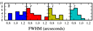
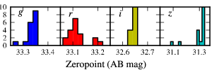
Figure 2.— The data were taken under a variety of conditions. These plots show the distribution in stellar FWHM (top) and photometric zeropoint (bottom) of the MegaCam images.

2.2. Data reduction

The MegaCam data were processed by the Elixer pipeline at CFHT. This facility applies standard bias subtraction, flat fielding and fringing corrections to the images. Elixer also determines a photometric solution based on standard fields observed over the same nights.

We used the Astromatic software scamp to determine an astrometric and relative photometric solution for each image and swarp to bring the images into pixel alignment (Bertin, 2006). Cosmic ray hits were detected and masked using the LACosmic IDL code (van Dokkum, 2001). Lastly, swarp was used to generate median stacked images.

Due to varying observing conditions, the data have a range in stellar point spread functions (PSFs) from 0.7-1.2″ full-width at half-maximum (FWHM). For robust aperture color measurements, we generated PSF-matched image stacks. We convolved each image with FWHM$<1\arcsec$ with a PSF-matched kernel. The kernel was determined by first fitting a Moffatt PSF model to high signal-to-noise stars for each of the 36 chips within the MegaCam focal plane. The kernel was then found that would result in a standard profile with FWHM=1″. In practice, the resulting convolved image has a FWHM$>1\arcsec$ due to tails in the PSF, and we find that PSF FWHM of the convolved images fall in the range from 1-1.2″. The masked regions, including defective pixels and cosmic ray hits, were also enlarged to account for the convolution.

We generated catalogs using SExtractor software (Bertin & Arnouts, 1996). The convolved images were processed in two-image mode to match the photometric apertures in each band. Source detection was performed on the $i$ images. We use the SExtractor mag_auto magnitudes to measure galaxy magnitudes and colors.

We investigated the completeness limits of the catalogs by adding artificial galaxies to the raw images and repeating the processing steps. The galaxies were modeled with $R^{1/4}$ exponential profiles with effective radii of $R_{e}=(0.5^{\prime\prime},1.0^{\prime\prime},1.5^{\prime\prime})$ matching the range in surface brightness of real sources. An artificial galaxy was said to be detected if the measured SExtractor magnitude was within 1 magnitude of the true value. The magnitude completeness limits for each field are listed for effective radius $R_{e}=1.0^{\prime\prime}$ in Table 1. Of note is field A which is shallow in $r$. The completeness limits are only directly relevant in $i$ band since we do not require significant detections in the other filters.

Field masks were constructed to exclude gaps in the detector, bad columns and the halos and diffraction spikes surrounding bright stars. Mask processing was facilitated by Mangle2 (Swanson et al., 2008).

2.3. Archival data

To determine the expected galaxy counts in the Cold Spot fields, we examined archival data available from the CFHT Legacy Survey (CFHTLS). We obtained catalogs and masks from data release 4, which includes 16 fields from the wide and deep surveys with $griz$ photometry. The field locations and areas are listed in Table 2. Field D1 overlaps W1 making the total survey area 9.8 sqr deg.

Both the CFHTLS Wide and Deep survey images are deeper than those of the Cold Spot. To account for this in our analysis, we degrade the photometry with Gaussian noise to match our Cold Spot fields.

Table 2CFHTLS Fields

		Area
ID	RA Dec	(sqr deg)
W1	02h20m –04d12m	6.69
W2	09h05m –02d23m	0.70
D1	02h25m –04d29m	0.77
D2	10h00m +02d12m	0.79
D3	14h19m +52d24m	0.83
D4	22h15m –17d43m	0.80

We can directly compare our own data with archival MegaCam fields with the caveat that the i-band filter was replaced since the beginning of the Legacy project. Our data were obtained with the new filter, designated i.MP9702, while the archival data are from the original i.MP9701 filter. The filter transmissions are sufficiently different that a color transform of order 0.1 magnitudes must be applied to compare the two data-sets.

When comparing i-band galaxy counts, we convert to the new i.MP9702 filter using the relation $i_{9702}=i_{9701}+0.078(r-i_{9701})$ derived from synthetic red galaxy photometry. We generate synthetic stellar and galaxy photometry using transmission functions obtained from S. Gwyn.

2.4. Sample selection

We found that due to residual zeropoint variations, additional corrections were warranted to obtain internally consistent stellar colors. Within each field, we fit the stellar loci in griz color space, see Fig. 3. Offsets of $\sim$0.05 magnitudes were applied to align the loci to model fits using the Pickles’ stellar library (Pickles, 1998). The typical errors in the alignment fits are: $\sigma_{g-r}=0.02$, $\sigma_{r-i}=0.01$ and $\sigma_{i-z}=0.01$ magnitudes. We applied color corrections to both Legacy and Cold Spot fields. We apply a dust extinction correction to extragalactic sources from Schlegel et al. (1998).

We classified sources as stars or galaxies based on the half-light radius in $i$ measured by SExtractor. We used the criteria presented in (Coupon et al., 2009) in which the cutoff is determined from a Gaussian fit to the distribution of radii for sources in the field. We classified sources to a limiting magnitude of $i_{9702}=21.5$; all fainter sources were treated as galaxies.

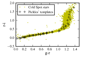
Figure 3.— We apply color corrections to align the stellar loci in $griz$ color space, illustrated here by the $g-r$,$r-i$ plot. Plotted are 2900 stars from the 7 Cold Spot fields. The plus symbols mark synthetic photometry from Pickles’ stellar SEDs.

We constructed a sample of red galaxies in $grz$ space. Due to the required photometric transform, we do not use the i-band for galaxy selection, ensuring that no selection bias arises between the Legacy and Cold Spot fields. The selection criteria are based on a passively evolving galaxy model (Bruzual & Charlot, 2003) and are illustrated in Fig. 4; the cuts are as follows. (1.) We defined a rotated color space $c_{1},c_{2}$ aligned with the red galaxy track at $z<0.4$ and impose a luminosity cut following the red sequence: $17<r<22.5$, $c_{1}=0.7(g-r)+3(1-0.7)(r-z-0.38)$, $c_{2}=(r-z)-(g-r)/3-0.38$, $c_{1}>0.294r-4.8$. (2.) The following cuts include low redshift ($z<0.4$) galaxies: $|c_{2}|<0.2$, $c_{1}<2.0$. (3.) High redshift galaxies are included with: $c_{2}>0.2$, $0.5<g-r<2.5$, $r-z<2.5$. The conservative $r<22.5$ cut was used to ensure that the sources were well detected in $r$, $i$ and $z$.

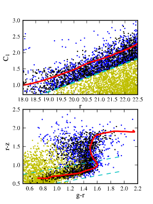
Figure 4.— The red galaxy sample was selected in $grz$ color space. At top: a luminosity cut was applied in $r$ following the evolutionary track. Bottom: cuts are made in $grz$ space. Overplotted is an evolutionary track for a passively evolving galaxy.

3. Magnitude-number relation

A coarse view of the galaxy distribution can be obtained from the differential galaxy count function with magnitude. Fig. 5 shows the i-band counts we measure in the Cold Spot fields including all sources classified as galaxies; the shaded region was measured from 16 CFHTLS fields over 9.8 sqr deg and represents the range of cosmic variance at the $\sim 2-\sigma$ level.

The Cold Spot fields are consistent with the Legacy fields. Of note are fields B and F, which show low number counts. Interestingly, F covers the low density spot in NVSS. The fields were not imaged under poor conditions, so there is no evidence that this is due to a systematic effect in completeness. Fields B and F are separated on the sky, so it is unlikely that the two measurements are related through a single large underdensity.

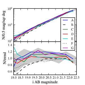
Figure 5.— The differential galaxy counts as a function of $i$-band magnitude. The top panel shows the counts per square degree in 0.5mag bins. The lines represent the 7 Cold Spot fields, A-G. The shaded region was measured from 15 CFHTLS fields and represents the range of cosmic variance. The bottom panel plots the same counts divided by the exponential trend. All fields are consistent with the CFHTLS data.

4. Redshift distribution

We use photometric redshifts to examine the galaxy distribution along the line of sight to the Cold Spot. The redshifts of early type galaxies can be estimated from broadband photometry based on the position of the 4000Å break (Connolly et al., 1995). The $gri$ colors constrain the redshift at $0.2<{\rm z}<0.4$ while the $riz$ colors primarily constrain the redshift at higher z, $0.4<{\rm z}<1.0$.

However, biases can arise from color-redshift degeneracies limiting the accuracy of photometric redshifts and introducing artificial features in the derived redshift distributions. We mitigate this by carrying out identical analysis procedures on both the Cold Spot and CFHTLS catalogs which we construct to have uniform photometric properties. We use the CFHTLS fields to find the expected mean counts, including the survey selection function and redshift error. We then use the redshift error estimates to deconvolve the photo-z distribution and find the underlying galaxy counts. The homogeneity of the data makes the procedure resilient to photo-z biases that may arise, for instance, from photometric uncertainty or from the limited spectroscopic calibration set. The methodology and results are described in the subsequent sections.

4.1. Photometric redshifts

We estimated galaxy redshifts using the griz photometry. We used the template fit photo-z algorithm eazy v1.00 (Brammer et al., 2008). The eazy code computes fits to photometric colors using linear combinations of galaxy SED templates and allows for magnitude-redshift priors. We used the built-in eazy template set which consists of six principal SED components with the appropriate MegaCam filter transmission curves. We added a broad $r$-band magnitude prior calibrated from the training set data as well, which is described below.

The spectroscopic sample consists of 928 galaxies from multiple surveys that overlap the CFHTLS fields, see Table 3. The redshift ranges and numbers listed include only sources within our red galaxy sample. We divided the sample into two sets of roughly 465 galaxies each to form separate training and validation sets.

Due to the luminosity cut there is a strong trend of galaxy magnitude with redshift within the red galaxy sample. To take advantage of this, we used the training sample to construct a magnitude-redshift prior. We adopted a functional form for the prior of $p(z|m)\propto z^{a}\exp[-(z/z_{0})^{a}]$ with parameters $a(m)$ and $z_{0}(m)$ tuned to match the mean and variance of the data. The mean and variance were fit as linear functions of magnitude; however, we artificially broadened the prior by scaling the variance by a factor of 4.

The model zeropoints can be inaccurate due to uncertainties in the instrumental transmission and photometric system. To improve the quality of the photo-z’s, we varied the color zeropoint offsets to optimize the fits. We iteratively ran the eazy code on the training set while varying the color zeropoint offsets using a simulated annealing optimization algorithm. The quality of the fit was measured by the root-mean-square error with 5-$\sigma$ outliers removed.

The results on the validation set is shown in Fig. 6. Here, Gaussian noise has been added to the CFHTLS photometry to model the Cold Spot data.

We used the full training set including artificial noise to estimate the photo-z error distribution. The error varies with redshift and may be biased. We fit the distribution in redshift bins of 0.1 with a two-Gaussian model. The error kernels are illustrated in Fig. 7.

Table 3Photo-z Training Set

Survey	CFHTLS Field	z-Range (Median z)	N
ZCOSMOS	D2	0.12–1.00 (0.47)	678
DEEP2	D3	0.20–0.98 (0.55)	125
VVDS	D1	0.14–0.88 (0.59)	111
SDSS LRG	D2,D3	0.31–0.38 (0.35)	14

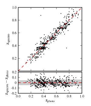
Figure 6.— The photometric redshift precision demonstrated on the validation set of $\sim 465$ galaxies. The photometry was degraded to model the photometric errors in the Cold Spot data. The shaded regions show $1-\sigma_{RMS}$ ranges.

4.2. Monte Carlo inversion

We modeled the underlying galaxy distribution with a Monte Carlo Markov Chain method. The model redshift distribution was constructed with four redshift bins from z=0.1-0.9, with $\Delta z=0.2$. We chose this coarse binning to minimize systematic errors, including uncertainties in the photo-z error kernel. The number of galaxies in each bin was treated as a parameter in the MCMC, giving four degrees of freedom. We evolved the chain using a random walk according to the Metropolis-Hastings algorithm.

At each step in the iteration, the true number of galaxies in each redshift bin was specified. The initial condition was set to the result of a Richardson-Lucy deconvolution and subsequent steps were then chosen in a random walk manner from a Gaussian proposal distribution. Additionally, proposed steps were required to give a positive number of galaxies in each bin.

The Monte Carlo photo-z distribution was constructed by distributing the model galaxies according to the photo-z error kernel. The likelihood of this distribution was then computed according to the Poisson distribution, $f(N_{i};\lambda_{i})$, with the mean, $\lambda$, set by the expected photo-z number counts from the archival data. Each proposed step was either accepted or rejected according to a likelihood ratio where the probability of accepting the $k^{th}$ step depends on the ratio of likelihoods, as,

$$p=\min\{\prod_{i}f(N_{i,k};\lambda_{i})/f(N_{i,k+1};\lambda_{i}),1\}$$ (1)

The chain converges quickly because only neighboring bins are strongly correlated. We carried out 50000 steps for each field and dropped the first 1000 iterations to ensure that the results are not affected by the starting condition.

We used the same MCMC procedure on the archival fields to determine the selection function. In this case, the galaxy counts from all 15 archival fields were summed and normalized by the total area. Fig. 7 illustrates the photo-z redshift distribution, along with a spline fit of the deconvolved distribution.

We normalized the galaxy counts by the selection function, and express the result as the overdensity, $N/\overline{N}-1$. The redshift distributions for the seven individual Cold Spot fields are shown in Fig. 8, along with the combined measurement from summing all of the fields. The likelihood function was found from the MCMC runs and arises from Poisson error. On top of this, there is a systematic uncertainty in the selection function determination. The plots also include a systematic error in the $r$ magnitude zeropoint of 0.05. This affects the two high redshift bins where the selection function is steeply falling. The added error is 1.5% in bin 3 and 6.1% in bin 4; in comparison, the Poisson errors in these bins are 3.7% and 4.7%, respectively. In the next section, we consider how color shifts affect the photo-z distribution as well.

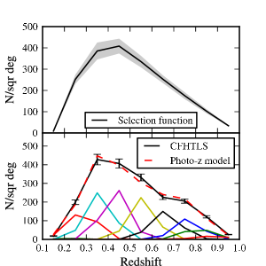
Figure 7.— Top: a spline fit of the deconvolved selection function. Bottom: the photo-z distribution (solid line) is well fit by the model selection function convolved with the photo-z error kernels (dashed line). The distribution decomposed into the photo-z error kernels is plotted along the bottom. The error bars represent uncertainty in the fit arising from cosmic variance.

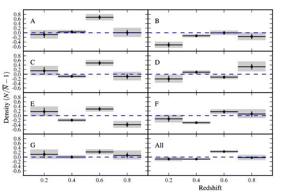
(a) (b) (c)

Figure 8.— Plotted are the corrected redshift number density distributions based on Monte Carlo modeling. Panel (a) shows the result from each of the 7 fields (A-G), as well as the mean distribution derived by summing the galaxy counts (All). The error bars give 68% marginalized likelihood ranges. Panel (b) shows the marginalized likelihood distribution of the density for the four redshift bins in the combined measurement. The filled histograms include systematic uncertainties in the selection function. The vertical shaded region is the 1-$\sigma$ range of cosmic variance and the arrow marks a 200Mpc diameter supervoid with underdensity $\delta=-0.3$. The typical normalized covariance between redshift bins is illustrated in Panel (c). Neighboring bins are anti-correlated by 20-40%.

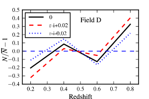
Figure 9.— To check the effect of systematic color offsets on the redshift distribution, we recomputed the photo-z’s with zeropoint offsets in $r$ of $\pm.02$ magnitudes. The plot shows the resulting measurement in field D. The distribution is shifted towards higher (+0.02) or lower (-0.02) redshift by the perturbations.

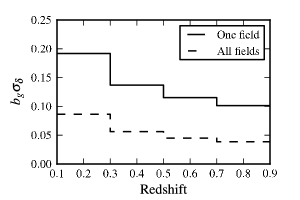
Figure 10.— The expected $1\sigma$ range in Gaussian density fluctuations in each redshift bin for one field and for all fields combined. We assume a linear galaxy bias of 1.5.

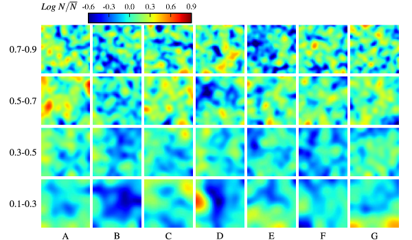
Figure 11.— Large structures are evident in the projected densities including two clusters at z=0.6 in field A, and an apparent void in field D in the same redshift bin. The density in each redshift bin is smoothed with a Gaussian kernel with a FWHM of 2Mpc. Each plot is 1° square. North is up and RA increases to the left. Masked regions excluding chip gaps and bright stars have been filled with a uniform distribution of galaxies according to the selection function.

4.3. Systematic uncertainties

A systematic variation in color or magnitude of sources between fields can significantly affect the derived photometric redshift distributions. Calibration errors in individual fields will tend to average out in the combined analysis, but a systematic difference between the archival and Cold Spot fields could strongly bias our conclusions. There are two primary issues: the magnitude zeropoint and color offsets.

The magnitude zeropoint affects the number of galaxies at high redshift through the $r$ magnitude limits and luminosity cut. We expect the photometric calibration from CFHT Elixer system to be better than 0.05 magnitudes and the offset due to the extinction correction is of the same order. We find that a shift of 0.05 magnitudes changes the sample size by 5% in the high redshift bins. This is is smaller than the Poisson error in number counts in a single field, but could bias the selection function. Based on the magnitude-number counts, as well as the redshift counts, we find no evidence for significant discrepancies. The zeropoint also affects the photometric redshifts through the magnitude prior, but this dependence is minor.

Variations in color between fields is more serious because these can redistribute galaxies in the photo-z distribution. The stellar loci alignment can be made to a precision of $r-i=.01$ magnitudes. The uncertainty in $g-r$ is greater, but has less of an effect on the photo-z estimates. Systematic uncertainties may come from the Galactic extinction correction as well, which has a similar order of $g-r\sim.02$. To test the effects of color shifts, we added an $r-i$ color offset of $\pm 0.02$ magnitudes and recomputed the redshift distribution. The result is a shift of the photo-z distribution to higher or lower redshift affecting number counts in bins by 10%, see Fig. 9. Though we do not expect such a large shift, this does limit the constraints we can put on the density especially in the lowest and highest redshift bins.

The redshift distributions in a number of fields show linear trends in Fig. 8, particularly fields C, D and E. In field D, due primarily to the first and last bins, the distribution shows a rising trend with increasing redshift, while field E shows the opposite trend. These features could be due to residual color zeropoint errors. There are also apparent oscillations in the number counts in fields D and E. The anti-correlations between bins may contribute to this, but these are properly accounted for in the MCMC procedure and represented in the marginalized error bars. A prominent feature is a significant overdensity at z=0.6 that appears in four of the seven fields and dominates the combined signal. This feature could be an artifact of the selection function perhaps due to an inaccurate photo-z model. We investigated how these features depend on the $r$ magnitude limit. With a deeper $r$ limit of 23.0, the redshift distributions are not significantly altered and the oscillations persist in fields D and E; however, the overdensity at z=0.6 is reduced, perhaps due to broader redshift errors. With a brighter limit of $r=22.0$, we detect few galaxies in the high redshift bin, but the prominent features in the distribution remain including the z=0.6 overdensity. We conclude that there are hints of systematic trends in the redshift distributions, but no significant features that can be addressed with the calibration methods available. We find that many of the features do indeed correspond to real structures, validating the redshift distributions.

5. Discussion

Structures are evident in the individual Cold Spot fields. The projected densities in bins of width $\Delta z=0.2$ are plotted in Fig. 11. There is an excess of sources at $z=0.6$ in field A, and we have confirmed by eye that there are indeed two clusters in the field.

Field B has a very significant underdensity of 60% in the first bin. This underdensity is confirmed in $i$ magnitude counts (Fig. 5) which are low for $i_{AB}<20$. Field F, which overlaps the NVSS depression identified by Rudnick et al. (2007), shows low magnitude counts as well and is underdense in the two low redshift bins by 10-30%. Thus, we conclude that the NVSS feature is due to an underdensity at $z<0.5$.

In field D, the underdensity at z=0.6 is resolved in R.A.-Dec. projection, suggesting that it is a real structure. This void is in the Northern part of field D, which has a width of $\sim 20$Mpc. We ran the 3D Voronoi tessellation-based void-finder zobov (Neyrinck, 2008) on all Cold Spot and CFHTLS fields, and this void has the largest density contrast of all voids found. However, it was necessary to severely distort the pencil beam into a compact shape (a cube) to use a Voronoi tessellation on the galaxies effectively, obscuring the physical meaning of this finding. The void is not seen in the adjacent field E, which has an overdensity in this bin, making it unlikely that field D is part of a larger supervoid.

The expected range in density due to cosmic variance is plotted in Fig. 10 for both a single field and the combined measurement. We assume a linear galaxy bias $b_{g}=1.5$. The underdensity at z=0.8 in field E is $-0.39$; this is a 3.8$\sigma$ deviation in terms of cosmic variance. The variations within fields are larger than expected: many of the fields deviate by $>2\sigma$ in at least one bin, and have a greater amplitude in the highest redshift bins. We find similar variations in the CFHTLS fields. We attribute the additional variance to systematic sources particularly affecting the lowest and highest bins. These issues make a robust void detection difficult in any single bin.

Additionally, void detections are limited by cosmic variance. Due to the limited sky coverage, a typical deviation due to small structures within a single field could be large enough to be consistent with a supervoid especially in the low redshift bins. However, we can detect a supervoid by looking for coherent structures across many fields. For instance, a 100Mpc radius void would reduce the number counts in most of the fields. Such a void with $\delta=-0.3$ would affect the galaxy density by $b_{g}\delta\sim-.45$. In a bin at z=0.6 with width $\Delta z=0.2$, the reduction in counts would be 15%. The arrows in Fig. 8(b) mark the expected underdensity due to this void in each redshift bin.

Using the combined likelihood distributions we can test the case of a supervoid with radius 100Mpc and $\delta=-0.3$. The density measurements in the four redshift bins and the expected decrement for this supervoid model are listed in table 4. We compute a likelihood, $p(<\delta)$, of measuring a density less than that of the supervoid based on the realizations in the MCMC chain.

At z=0.2, we measure an underdensity of 8.5% which is consistent with the supervoid. The underdensity at z=0.4 is not deep enough to match the void model at the 97% confidence level, neglecting systematic uncertainties in the selection function. We find an overdensity at z=0.6, and the measured number density in the last bin, at z=0.8, is inconsistent with the supervoid at the 99.7% level.

We note that the 140Mpc empty void model proposed by Rudnick et al. (2007) is inconsistent with our measured redshift distribution at the level of 1 in 50000 in each redshift bin and can be ruled out.

Table 4Supervoid model limits

Redshift	$N/\overline{N}-1$	$(N/\overline{N}-1)_{model}$	$p(<\delta)$
0.1-0.3	-0.085	-0.12	0.25
0.3-0.5	-0.088	-0.13	0.029
0.5-0.7	0.24	-0.15	$<1e-5$
0.7-0.9	-0.022	-0.17	0.0026

Do the underdensities measured at $z<0.5$ provide evidence for a supervoid? The deviation of 8.5% in the first bin is only a $1.0\sigma$ fluctuation in terms of cosmic variance. This alone suggests that it is an unlikely source of the Cold Spot since it is a typical fluctuation. It is predominantly detected in only fields B, D and F, but not in adjacent field E. Furthermore, the only fields that also show a low magnitude-number relation are B and F. It is likely that a large underdensity would not be homogeneous, but the data do not provide overwhelming evidence for a coherent large structure. The underdensity at z=0.4 is interesting because it is measured in four of the seven fields. It is a $1.6\sigma$ deviation with respect to cosmic variance. This provides a hint of a large structure, but more sky area is required to make a robust measurement.

Smaller voids may extend over a subset of the fields. At z=0.2, fields B, D and F are particularly underdense with an angular extent of 5° or 50Mpc at this redshift. However, the linear ISW temperature decrement predicted for a 50Mpc diameter volume is 0.3$\mathrm{\mu K}$. At z=0.4, a structure with the same angular extent would be 100Mpc in diameter and produce a 0.9$\mathrm{\mu K}$  decrement. It is unlikely that even having many of these modest supervoids along the line of sight could produce the Cold Spot feature.

The significant overdensity at z=0.6 measured in four of the fields could represent a massive structure. The 25% overdensity is consistent with a 200Mpc diameter overdensity with $\delta=0.5$. To linear order, this would induce a 5$\mathrm{\mu K}$ hot spot on the CMB. This suggests that the primary anisotropy on the CMB is even colder than observed. Overdensities can induce cold spots due to the non-linear Rees-Sciama effect which comes to dominate at high redshift (Sakai & Inoue, 2008), but this is thought to be important only at $z>1$.

6. Conclusions

We investigated the distribution of galaxies at $z<0.9$ in the direction of the CMB Cold Spot. We detect an underdensity at low redshift, $0.1<z<0.3$, that is consistent with the density expected from a supervoid. This underdensity appears to be present in 2MASS as well (Francis & Peacock, 2009). However, due to the limited sky coverage of our survey, we cannot draw a definite conclusion regarding the existance of a coherent supervoid structure. Our measurements disfavor a supervoid with $\delta=-0.3$ at z$=0.3-0.5$, and we can rule out a supervoid at $z=0.5-0.9$. We must be cautious in interpreting the density measurements due to possible systematic shifts in the selection function, especially in the near and far redshift bins.

In Granett et al. (2008, 2009) we found the imprint of supervoids in SDSS to be stronger than predicted from linear ISW. This suggests that a more modest supervoid with $\delta\gtrsim-0.3$ could be the origin of the Cold Spot decrement.

Significant progress will be made in understanding the Cold Spot with wide-area large-scale structure surveys including Pan-STARRS-1 (Kaiser, 2004). Additionally, polarization data from the Planck mission (White, 2006) may provide additional information on the intrinsic CMB fluctuations in this area.

References

- Adelman-McCarthy et al. (2008) Adelman-McCarthy, J. K. et al. 2008, ApJS, 175, 297, arXiv:0707.3413
- Bennett et al. (2003) Bennett, C. L. et al. 2003, ApJS, 148, 1, arXiv:astro-ph/0302207
- Bertin (2006) Bertin, E. 2006, in Astronomical Society of the Pacific Conference Series, Vol. 351, Astronomical Data Analysis Software and Systems XV, ed. C. Gabriel, C. Arviset, D. Ponz, & S. Enrique, 112–+
- Bertin & Arnouts (1996) Bertin, E., & Arnouts, S. 1996, A&AS, 117, 393
- Brammer et al. (2008) Brammer, G. B., van Dokkum, P. G., & Coppi, P. 2008, ApJ, 686, 1503, 0807.1533
- Bruzual & Charlot (2003) Bruzual, G., & Charlot, S. 2003, MNRAS, 344, 1000, arXiv:astro-ph/0309134
- Connolly et al. (1995) Connolly, A. J., Csabai, I., Szalay, A. S., Koo, D. C., Kron, R. G., & Munn, J. A. 1995, AJ, 110, 2655, arXiv:astro-ph/9508100
- Coupon et al. (2009) Coupon, J. et al. 2009, A&A, 500, 981, 0811.3326
- Cruz et al. (2005) Cruz, M., Martínez-González, E., Vielva, P., & Cayón, L. 2005, MNRAS, 356, 29, arXiv:astro-ph/0405341
- Cruz et al. (2008) Cruz, M., Martinez-Gonzalez, E., Vielva, P., Diego, J. M., Hobson, M., & Turok, N. 2008, ArXiv e-prints, 804, arXiv:0804.2904
- Cruz et al. (2006) Cruz, M., Tucci, M., Martínez-González, E., & Vielva, P. 2006, MNRAS, 369, 57, arXiv:astro-ph/0601427
- Davis et al. (2003) Davis, M. et al. 2003, in Society of Photo-Optical Instrumentation Engineers (SPIE) Conference Series, Vol. 4834, Society of Photo-Optical Instrumentation Engineers (SPIE) Conference Series, ed. P. Guhathakurta, 161–172
- Francis & Peacock (2009) Francis, C. L., & Peacock, J. A. 2009, ArXiv e-prints, 0909.2495
- Górski et al. (2005) Górski, K. M., Hivon, E., Banday, A. J., Wandelt, B. D., Hansen, F. K., Reinecke, M., & Bartelmann, M. 2005, ApJ, 622, 759, astro-ph/0409513
- Granett et al. (2008) Granett, B. R., Neyrinck, M. C., & Szapudi, I. 2008, ApJ, 683, L99, arXiv:0805.3695
- Granett et al. (2009) ——. 2009, ApJ, 701, 414, 0812.1025
- Inoue & Silk (2007) Inoue, K. T., & Silk, J. 2007, ApJ, 664, 650, astro-ph/0612347
- Kaiser (2004) Kaiser, N. 2004, in Society of Photo-Optical Instrumentation Engineers (SPIE) Conference Series, Vol. 5489, Society of Photo-Optical Instrumentation Engineers (SPIE) Conference Series, ed. J. M. Oschmann, Jr., 11–22
- Le Fèvre et al. (2005) Le Fèvre, O. et al. 2005, A&A, 439, 845, arXiv:astro-ph/0409133
- Lilly et al. (2009) Lilly, S. J. et al. 2009, ApJS, 184, 218
- Maturi et al. (2007) Maturi, M., Dolag, K., Waelkens, A., Springel, V., & Enßlin, T. 2007, A&A, 476, 83, arXiv:0708.1881
- McEwen et al. (2007) McEwen, J. D., Vielva, P., Hobson, M. P., Martínez-González, E., & Lasenby, A. N. 2007, MNRAS, 376, 1211, arXiv:astro-ph/0605122
- Neyrinck (2008) Neyrinck, M. C. 2008, MNRAS, 386, 2101, 0712.3049
- Pickles (1998) Pickles, A. J. 1998, PASP, 110, 863
- Rees & Sciama (1968) Rees, M. J., & Sciama, D. W. 1968, Nature, 217, 511
- Rudnick et al. (2007) Rudnick, L., Brown, S., & Williams, L. R. 2007, ApJ, 671, 40, arXiv:0704.0908
- Sachs & Wolfe (1967) Sachs, R. K., & Wolfe, A. M. 1967, ApJ, 147, 73
- Sakai & Inoue (2008) Sakai, N., & Inoue, K. T. 2008, Phys. Rev. D, 78, 063510, arXiv:0805.3446
- Schlegel et al. (1998) Schlegel, D. J., Finkbeiner, D. P., & Davis, M. 1998, ApJ, 500, 525, arXiv:astro-ph/9710327
- Smith & Huterer (2010) Smith, K. M., & Huterer, D. 2010, MNRAS, 403, 2
- Swanson et al. (2008) Swanson, M. E. C., Tegmark, M., Hamilton, A. J. S., & Hill, J. C. 2008, MNRAS, 387, 1391, 0711.4352
- van Dokkum (2001) van Dokkum, P. G. 2001, PASP, 113, 1420, arXiv:astro-ph/0108003
- Vielva et al. (2004) Vielva, P., Martínez-González, E., Barreiro, R. B., Sanz, J. L., & Cayón, L. 2004, ApJ, 609, 22, arXiv:astro-ph/0310273
- White (2006) White, M. 2006, New Astronomy Review, 50, 938, arXiv:astro-ph/0606643
- Zhang & Huterer (2010) Zhang, R., & Huterer, D. 2010, Astroparticle Physics, 33, 69, 0908.3988