A scientific understanding of network designing

Abstract

As the Internet becomes severely overburdened with exponentially growing traffic demand, it becomes a general belief that a new generation data network is in urgent need today. However, standing at this crossroad, we find that we are in a situation that lacks a theory of network designing. This issue becomes even more serious as the recent progress of network measurement and modeling challenges the foundation of network research in the past decades.

This paper tries to set up a scientific foundation for network designing by formalizing it as a multi-objective optimization process and quantifying the way different designing choices independently and collectively influence these objectives. A cartesian coordinate system is introduced to map the effect of each designing scheme to a coordinate. We investigated the achievable area of the network designing space and proved some boundary conditions. It is shown that different kind of networks display different shapes of achievable areas in the cartesian coordinate and exhibit different abilities to achieve cost-effective and scalable designing. In particular, we found that the philosophy underlying current empirical network designing and engineering fails to meet the cost-effective and evolvable requirements of network designing. We demonstrated that the efficient routing combined with effective betweenness based link bandwidth allocation scheme is a cost-effective and scalable design for BA-like scale-free networks, whereas if other designing choices cannot be determined beforehand, ER network is a markedly good candidate for cost-effective and scalable design.

I Introduction

The Internet becomes more and more complex and susceptible to congestion today. With the emergence of new data-intensive applications and fast growing population in need of data communication service, most experts agree that the existing data network architecture is severely stressed and approaching its capability limits[1, 2, 3, 4]. Thus the move to a brand new next generation data network is in urgent need today.

However, before this move, there lacks the theory of network designing, which becomes more serious as the recent surge of network measurement and modeling efforts show quite counter-intuitive result, that is, most networks, including the Internet, display scale-free structures rather than presumably random structures[5, 6, 7, 9]. This recent trend poses an urgent need as well as an opportunity for a fundamental understanding of the science underlying the network designing. The Network Science and Engineering Council(NetSE) has recommended the creation of “a fundamental science of networking that has the potential to underpin systematic engineering methodologies for the design of large-scale, robust, cost-effective and evolvable networked systems” to be among the top agenda for long-term network research [11]. The hardness of establishing this science primarily lies in the abstraction of network designing. Too simple model may lose its practicality, while too complicated model that includes too many details may lead to insolvability. At the heart of various designing considerations, a scientific approach should clarify the following key issues: what are the typical network designing objectives and major designing choices, what are the inherent interplays of these choices, how the designing choices independently and collectively affect different designing objectives, and what are the achievable values of the designing objectives.

From the macroscopic perspective, network designing often involves several independent yet closely related aspects, of which the three most fundamental ones are what kind of network topology shall be used, which routing algorithm is effective, and how the link bandwidth will be allocated. One can independently choose either ingredients as they are conceptually orthogonal to each other. However, when network designing objectives are concerned, these ingredients become closely interleaved because different combinations will produce different effects.

One major objective for network designing and engineering is to enhance the network’s transmission capacity, a focus of a number of previous researches[12, 13, 20, 21, 22, 14]. However, we argue that most often, maximizing the network transmission capacity could not be the sole objective. A network designing is also typically constrained by the financial or technical restrictions, so a cost-effective design is preferable. In addition, as networks are constantly evolving, a designing scheme with good scalability will be more desirable. To summarize, previous researches have the following shortcomings : (1) they focus only on one aspect of the network designing ingredients, without a formally defined scientific framework ; (2) their studies are based on a traffic flow model that is too simple for network engineering; (3) they don’t consider the technical feasibility of the designing scheme, which is crucial for network engineering; (4) they do not consider the scalability issue of a designing scheme, which is of significance in reality because networks are constantly evolving.

Motivated by these incentives, in this paper, we carried out an in-depth study of network designing in a systematic approach. The main contributions are:

1. We propose that network designing is a multi-objective optimization process, with often contradictive objectives, and formalize the framework for network designing study by defining a two dimensional cartesian coordinate system according to the two important designing objectives;

2. We compare different designing schemes by quantitatively mapping the effect of each scheme to a coordinate in the coordinate system, and we explore the achievable areas in this coordinate system;

3. We investigate the cost-effectiveness and scalability of some representative designing schemes. In particular, we find that the current network designing philosophy is neither cost-effective nor scalable. We propose one cost-effective and scalable designing scheme, i.e., efficient routing combined with effective betweenness based bandwidth allocation, which can achieve pretty good tradeoff between the two designing objectives for BA-like scale free networks, and we demonstrate that if one has the full freedom to select network designing choices, ER network is a remarkably good candidate to achieve a cost-effective and scalable design, especially when other designing ingredients cannot be determined beforehand.

The subsequent paper is structured as follows: We briefly review related work in Section II and introduce our modified traffic flow model in section III. The major network designing objectives and designing choices are presented in section IV. We move forward to the definition and analytical analysis of the cartesian coordinate system and achievable areas in section V. The scalability issue of network designing is discussed in section VI. Finally, we conclude the paper in section VII

II Related Work

The past decade has witnessed a surge of network topology measurement and modeling research activities[5, 6, 24, 23, 25, 26, 27, 8, 10], which, with abundant evidence, show that most real networks, including the Internet, display scale-free network structure. This milestone finding challenges the foundation of network related studies, since for decades the network researches are grounded on the general assumption of random network model [33].

Recently, there is a research shift from the static network topology characterization and modeling to the traffic dynamics on these new networks[19, 12, 13, 20, 21, 22, 14]. These work, primarily for enhancing the network’s transmission capacity, can be broadly classified into three categories: to make small changes to the underlying network topology[12, 13, 20], to adjust the routing algorithm[21] and to customize the node capability[22, 14]. A straightforward way to improve the network’s transmission capacity is to create new edges in the network[12, 13]. A somewhat counter-intuitive approach proposed in [20] is to enhance the BA network’s transmission capacity by removing edges that connect nodes with high betweenness values, hence balancing the traffic across the network. In [21], the authors try to achieve the same goal by the so called efficient routing algorithm. Instead of routing packets along the path with minimum number of hops, efficient routing routes packets along the path that minimizes the sum of node degrees, hence bypassing those high degree nodes in BA network. In [22], the authors investigate this issue from yet another angle, i.e., to adjust the node capability. Two node capability models are studied in this work, i.e., with node capability proportional to its degree and betweenness respectively. These two capability models are further investigated under the condition that the total capability remains fixed[14, 15], which essentially turns the problem of node capability assignment to an optimization problem. A central concept behind these analysis is the betweenness centrality[32, 16, 17, 18], which bridges the research of static network topology and dynamic network traffic analysis. Under certain circumstances, the betweenness centrality precisely estimates the traffic passing through a node or an edge[16, 17, 18, 21].

III Traffic flow model

In this study, we use a traffic-flow model that is slightly different from [21, 20, 22, 28] to more accurately model the network realism. Each node is capable of generating, forwarding and receiving packets. At each time step, $R$ packets are generated at randomly selected sources. The destinations are also chosen randomly. Instead of assigning a single node capability to each node as previous studies do, we assign multiple link bandwidths to multiple interfaces of each node. Denote $C(v_{i})$ to be the link bandwidth of the $i$th interface of node $v$, then $C(v_{i})$ specifies the maximal number of packets this interface can deliver at a time step. We assume symmetric link bandwidth, i.e., for an edge $e=(v_{i},u_{j})$, we have $C(v_{i})=C(u_{j})$, which is further denoted as $C(e)$. Each packet is forwarded toward its destination based on the particular routing algorithm used. When the total number of arrived and newly created packets to be delivered at interface $v_{i}$ exceeds $C(v_{i})$, the packets are stored in this interface’s queue and will be processed in the following time steps on a first-in-first-out(FIFO) basis. If there are several candidate paths for one packet, one is chosen randomly. Each interface has a queue for delivering newly arriving packets. Packets reaching their destinations are deleted from the system. As in [21, 20, 22, 28], interface buffer size in this traffic-flow model is set as infinite as it is not relevant to the occurrence of congestion.

For small values of the packet generating rate $R$, the number of packets on the network is small so that every packet can be processed and delivered in time. Typically, after a short transient time, a steady state for the traffic flow is reached where, on average, the total numbers of packets created and delivered are equal, resulting in a free-flow state. For larger values of $R$, the number of packets created is more likely to exceed what the network can process in time. In this case traffic congestion occurs. As $R$ is increased from zero, we expect to observe two phases: free flow for small $R$ and a congested phase for large $R$ with a phase transition from the former to the latter at the critical packet-generating rate $R_{c}$.

In order to measure $R_{c}$, we use the order parameter [31] $\eta=\lim_{t\rightarrow\infty}{{\langle\Delta\Theta\rangle}\over{R\Delta t}}$, where $\Theta(t)$ is the total number of packets in the network at time $t$, $\Delta\Theta=\Theta(t+\Delta t)-\Theta(t)$, and $\langle\cdots\rangle$ indicates the average over time windows of $\Delta t$. For $R<R_{c}$ the network is in the free-flow state, then $\Delta\Theta\approx 0$ and $\eta\approx 0$; and for $R>R_{c}$, $\Delta\Theta$ increases with $\Delta t$ thus $\eta>0$. Therefore in our simulation we can determine $R_{c}$ as the transition point where $\eta$ deviates from zero.

TABLE I: Elementary topological properties of the five networks, each containing 1200 nodes. $N$ and $M$ denote the number of nodes and number of edges respectively, $D$ denotes the diameter, $L$ denotes the average shortest path length.

Network	$N$	$M$	$D$	$L$
WS	1200	2400	15.5	7.86
ER	1200	2450	11	5.23
BA	1200	2390	8	4.43
PA	1200	2400	8.7	4.03
HOT	1200	2583	9	5.16

IV Network designing choices and objectives

Of the various network designing choices, the following three ones are of critical relevance: routing algorithm, link bandwidth allocation scheme, and network topology. Designers could be faced with different scenarios characterized by the choices he can make. For example, when designing a brand new network from the very beginning, designers own the full freedom of choosing each ingredient, while when improving an existing network, designers can only change the routing algorithm or upgrade the link bandwidth.

A specific designing is often associated with explicit designing objectives. In this paper, we consider three major network designing objectives: the network transmission capacity, which should be as large as possible, the maximal bandwidth required to realize the designing scheme, which should be as small as possible, and the scalability, which should be as scalable as possible.

Enhancing network transmission capacity is one of the major goals for network designing and engineering, and is typically measured by the critical packet-generating rate $R_{c}$ [21, 20, 22, 28]. Although a simulation-based approach is feasible to measure $R_{c}$, it is time-consuming. The betweenness centrality provides a means to analytically evaluate the $R_{c}$ under the shortest path routing algorithm.

In our modified model, for any given network under shortest path routing, the expected number of packets passing through an edge is $\frac{RB(e)}{N(N-1)}$ at one time step, with each half flowing towards one direction, where B(e) is the betweenness centrality of the edge $e$. So for interface $v_{i}$ not to get congested, it follows that $\frac{1}{2}\cdot\frac{RB(e)}{N(N-1)}\leq C(v_{i})$, which leads to $R\leq\frac{2C(v_{i})N(N-1)}{B(e)}$. As a result, the critical packet generating rate $R_{c}$ for shortest path routing is:

$$R_{c}=min_{e\in E}\frac{2C(e)N(N-1)}{B(e)}$$ (1)

where $E$ corresponds to the edge set of the network.

In the more general situation, for any topology-based routing algorithm $\Gamma$, we introduce the effective betweenness $B^{\Gamma}(e)$ (similar to the definition in [21]) to estimate the possible traffic passing through an edge under routing algorithm $\Gamma$, which is formally defined as:

$$B^{\Gamma}(e)=\sum_{u,v\in V,u\neq v}\frac{\delta^{\Gamma}_{(e)}(u,v)}{\delta^{\Gamma}(u,v)}$$

where $V$ is the node set, $\delta^{\Gamma}(u,v)$ is the total number of candidate paths between node $u$ and $v$ under routing algorithm $\Gamma$, and $\delta^{\Gamma}_{(e)}(u,v)$ is the number of candidate paths that pass through edge $e$ between $u$ and $v$ under routing algorithm $\Gamma$.

Following this definition, the critical packet generating rate $R_{c}$ under routing algorithm $\Gamma$ can be calculated as:

$$R_{c}=min_{e\in E}\frac{2C(e)N(N-1)}{B^{\Gamma}(e)}$$ (2)

This equation also explains how different designing ingredients affect the $R_{c}$. $C(e)$ represents the bandwidth allocation scheme, and $B^{\Gamma}(e)$ is the collective effect of network topology and routing algorithm.

The maximal bandwidth, denoted as $C_{max}$, required to realize the $R_{c}$ is another designing objective of particular importance to network designing and engineering, because it directly relates to the technical feasibility(sometimes also monetary issue) of the specific designing scheme. By posing an upper bound of the required link bandwidth, it can be used to judge whether the proposed designing scheme can be realized with state-of-art technologies or available monetary budget.

Scalability is an issue that becomes increasingly important because today’s networks are all large-scale and constantly evolving. A scalable designing will have long-term benefit for the network investors and operators. In this study, the scalability will be measured by the growth trends of $R_{c}$ and $C_{max}$.

TABLE II: Theoretical result of the critical packet-generating rate $R_{c}$ under different combinations for networks in Table I. The result is obtained from Equation 2. For each kind of network, we generate 10 instances, and the result is the average of the 10 instances.

(bandwidth allocation scheme, routing algorithm)	BA	PA	HOT	ER	WS
(UC, SPR)	88.5	92.8	99.1	284.5	111.1
(UC, EFR)	264.3	195.3	94.6	390.6	147.9
(BC, SPR)	1079.4	1192.2	1001.7	937.9	610.2
(EBC, EFR)	766.6	844.9	909.2	891.4	606.2

TABLE III: Simulation result of the critical packet-generating rate $R_{c}$ under different combinations for BA, PA, HOT, ER and WS networks. For each kind of network, 10 instances are generated and for each instance, we run ten simulations. The result here is the average over all the simulations. Compared with Table III, it is shown that the simulation result is roughly consistent with the theoretical analysis.

(bandwidth allocation scheme, routing algorithm)	BA	PA	HOT	ER	WS
(UC, SPR)	110.2	115.6	119.9	370.5	136.7
(UC, EFR)	320.4	249.6	114.6	519.8	174.7
(BC, SPR)	934.2	1042.7	840.8	844.2	517.0
(EBC, EFR)	678.0	741.0	768.2	809.9	519.9

TABLE IV: $C_{max}$ under different combinations of network topologies, routing algorithms and bandwidth allocation schemes. It is evident that betweenness based link bandwidth allocation scheme often incurs high $C_{max}$, especially for heterogenous networks. Although (EBC,EFR) can assure much lower $C_{max}$ for BA-like scale-free networks, the reduction is not apparent for HOT network.

(bandwidth allocation scheme, routing algorithm)	BA	PA	HOT	ER	WS
(UC, *)	1	1	1	1	1
(BC, *)	12.43	12.99	10.30	3.37	5.63
(EBC, EFR)	2.91	4.45	9.70	2.40	4.13

Two typical routing algorithms are investigated in this paper: the shortest path routing, abbreviated as SPR, and the efficient routing[21], abbreviated as EFR. More formally, the efficient routing chooses a path $s=v_{0},v_{1},v_{2},\cdots,v_{k}=t$ between $s$ and $t$ that minimizes the objective function $\sum_{0\leq i<k}d(v_{i})$, where $d(v_{i})$ is the vertex degree of $v_{i}$.

Three link bandwidth allocation schemes are analyzed: the uniform link bandwidth allocation scheme, denoted as UC, the betweenness based link bandwidth allocation scheme, denoted as BC , and the effective betweenness based link bandwidth allocation scheme, denoted as EBC. In UC, each link has the same bandwidth, while in BC and EBC, each link’s bandwidth is proportional to its edge betweenness and effective betweenness respectively. For the purpose of comparing between different bandwidth allocation schemes, we keep the condition that the total link bandwidth assigned to all edges remains fixed, which is set to the number of edges in the network, i.e., $\sum_{e}B(e)=M$. The BC scheme is also investigated in [22], but it is not treated as an optimization problem because the total link bandwidth is not fixed.

Thus, if the network topology is predetermined, a designing scheme is a combination of routing algorithm and link bandwidth allocation scheme. When network topology is undetermined, it becomes another ingredient of the designing scheme. We investigate five network topologies in this paper: BA[6], HOT[29], ER[33], WS[34], and PA. BA network is constructed according to the standard BA model with $m=2$. ER network is constructed by the $G_{n}(p)$ model with the constraint of connectedness. WS network is built from the ring by randomly rewiring 15 percent of its edges, also with the constraint of connectedness. PA is indeed a variant of the BA model, and is generated by the following process: begin with 3 fully connected nodes, and add one new node to the graph in successive steps, such that this new node is connected to the existing nodes with probability proportional to the current node degree, and finally, add some internal edges to augment the graph by selecting both endpoints with probability proportional to the current node degree. The main difference between PA and BA is that PA has the rich-club structure[30], while BA does not. Finally, the HOT network is a heuristically optimal topology for the Internet router-level network, which can be roughly partitioned into three hierarchies: the low degree core routers, the high degree gateway routers hanging from the core routers, and the low degree periphery nodes connected with the gateway routers. The HOT networks generated here follow the same degree distributions as the corresponding PA networks. The basic network properties of these networks of size 1200 are presented in Table I.

V The cartesian coordinate system and achievable areas

For a given network, the effect of a designing scheme can be mapped to a coordinate in the cartesian coordinate system, with $C_{max}$ being the $X$-axis and $R_{c}$ being the $Y$-axis. A natural question is what are the value domains of $C_{max}$ and $R_{c}$.

It is easy to see that $C_{max}$’s value range is [1, M]. The optimal (smallest) value is achieved with uniform bandwidth allocation scheme, and the largest is achieved by allocating all the bandwidth to a single edge.

Regarding $R_{c}$, the lower bound is 0, which can be achieved by some loop based routing algorithms, that is, the packets are always looping in the network.

The upper bound $R_{c}$ is given by the following Theorem.

Theorem 1.

Given a network $G$, the upper bound $R_{c}$ for any designing scheme is $2M/L$, where $L$ is the average shortest path length of $G$; and, this upper bound is only achieved with (BC, SPR).

Proof:

The general idea of the proof is that the number of packets generated at each time step cannot exceed the maximal number of packets the network can consume at each time step. Since the total link bandwidth is $M$, the sum of interface bandwidth is $2M$, which means the network can at most forward $2M$ packets one step towards their destinations. Because each packet is generated with random source and destination, the expected number of steps needed to move one packet from the source to its destination under routing algorithm $\Gamma$ is $L^{\Gamma}$, which is equivalent to say that the network can consume at most $2M/L^{\Gamma}$ packets at each time step. So, we have

$$R_{c}\leq 2M/L^{\Gamma}\leq 2M/L$$ (3)

which means $2M/L$ is an upper bound of $R_{c}$.

Then we prove that (BC, SPR) can indeed achieve this upper bound $R_{c}$. Recall that $R_{c}=min_{e\in E}\frac{2C(e)N(N-1)}{B(e)}$, which in (BC, SPR), can be rewritten as:

$$\begin{split}R_{c}&=min_{e\in E}\frac{2C(e)N(N-1)}{B(e)}\\ &=min_{e\in E}\frac{2B(e)/\sum_{f\in E}B(f)\times M\times N(N-1)}{B(e)}\\ &=\frac{2MN(N-1)}{\sum_{f\in E}B(f)}\\ &=\frac{2MN(N-1)}{N(N-1)L}\\ &=\frac{2M}{L}\end{split}$$

This proves that the upper bound $2M/L$ is achievable.

Finally, we prove that (BC,SPR) is the only scheme that achieves $R_{c}=2M/L$. According to the Inequality 3, only when two conditions hold simultaneously can $R_{c}$ reach $2M/L$. These two conditions are: (1)$L^{\Gamma}=L$, which implies that the routing algorithm is SPR, and (2) the network can on average move $2M$ packets one step toward their destinations. Because in SPR, the expected number of packets arriving at interface $v_{i}$ in free flow state is exactly $\frac{1}{2}\frac{RB(e)}{N(N-1)}$, where $e$ is incident edge of interface $v_{i}$. When $R=2M/L$, the average total number of packets in the network is $\sum_{e}\frac{RB(e)}{N(N-1)}=2M$. So, for the whole network to move $2M$ packets at each time step, each interface should exactly move $\frac{MB(e)}{N(N-1)L}$ packets at each time step, which corresponds to the BC link bandwidth allocation scheme. ∎

In fact, (BC, SPR) reflects the conventional basic philosophy of real-world empirical network designing. Real-world network routing protocols such as OSPF and BGP are often based on shortest path routing(or at least making path length a major decision factor in path selection). High bandwidth links are placed at key points of the network, and when some links get overburdened, they will be upgraded by links with higher bandwidth, potentially attracting even more traffic and incuring a vicious cycle in traffic demanding and link bandwidth upgrading.

(a) BA

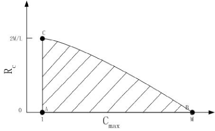
(b) Regular Networks

Figure 1: Illustration of the achievable areas for (a) BA-like networks, and (b) regular networks

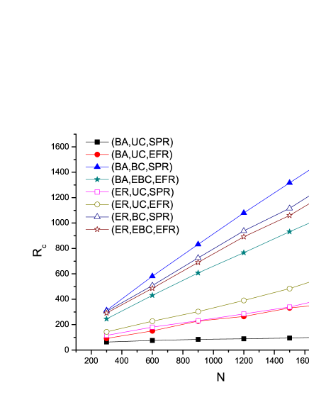
(a) $R_{c}$

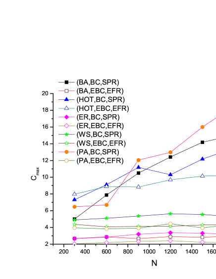
(b) $C_{max}$

Figure 2: (Color online) Scalability of (a)$R_{c}$ values of BA, HOT and ER under four different configurations; and (b) $C_{max}$ values of BA and ER under (BC,SPR) and (EBC, EFR) schemes.

Theorem 1 also implies that the optimal $R_{c}$ and optimal $C_{max}$ cannot be achieved at the same scheme, except for complete homogenous regular networks, indicating the presence of a tradeoff issue, which is confirmed by Table II(with the simulation result of $R_{c}$ presented in Table III) and Table IV.

It can be seen that although (BC,SPR) can guarantee highest $R_{c}$, it often incurs high $C_{max}$, because $C_{max}=\frac{MB_{max}}{N(N-1)L}$ is proportional to the largest betweenness, which is especially large for heterogenous networks. Hence, (BC,SPR) is not a cost-effective design for heterogenous networks. A consequently natural question is what is the achievable $R_{c}$ with the lowest $C_{max}$.

With (UC, SPR), it is easy to show that $R_{c}=\frac{2N(N-1)}{B_{max}}$. For regular networks such as ring and toroidal lattice, (UC, SPR) achieves the same $R_{c}$ as (BC,SPR), however, for heterogenous networks, $B_{max}$ can be quite large so that its $R_{c}$ will be significantly dwarfed compared with $R_{c}$ in (BC, SPR)(see Table II and Fig. 2(a)).

In BA-like scale-free networks, this $R_{c}$ can be improved by changing the routing algorithm from SPR to EFR (see Table II and Table III). Indeed, the $R_{c}$ in (UC,EFR) is $R_{c}=\frac{2N(N-1)}{B^{(EFR)}_{max}}$, where $B^{(EFR)}_{max}$ is the largest effective betweenness centrality among all edges. While EFR can significantly improve BA-like network’s transmission capacity because $B^{(EFR)}_{max}$ is substantially decreased compared with $B_{max}$, it is ineffective for the more realistic HOT model and WS network, and less effective for the ER network(see Table II).

It is evident that there is an optimal $R_{c}$ at the lowest $C_{max}$. It is easy to demonstrate the existence of such a routing algorithm that will realize this $R_{c}$, but it is not an easy task to find a practically implementable routing algorithm. Recall that with UC, $R_{c}=\frac{2N(N-1)}{B^{\Gamma}_{max}}$, so the essence to realize the optimal $R_{c}$ at UC is to find a routing algorithm that minimizes the $B^{\Gamma}_{max}$, which is equivalent to find a path set of size $N(N-1)$, containing exactly one path for each node pair, such that the maximal per edge occurrence in this path set is minimized. The intended path set can be found by firstly computing all the simple paths between any node pairs, and then enumerating all combinations of such path set. However, this approach in reality is infeasible for even median sized networks. A greedy heuristic algorithm that works can be as follows:

1. compute all the simple paths between any node pairs;

2. construct an initial path set, for example, the path set induced by the shortest path routing or efficient routing;

3. for any node pair, if there is a path such that if replacing this path with the present one in the path set will reduce the maximal per edge occurrence, replace the present path with this path. Repeat this step until there is no such path.

In reality, this routing algorithm is impractical. The significance of this scheme is that it is a key point in shaping the skeleton of the achievable area.

An illustration of the achievable area for BA-like scale-free networks is shown in Fig. 1(a), in which the four typical designing schemes are marked. The other three points A, B and C, which are important for a conceptual bounding of the achievable area are also illustrated, where A is a scheme that combines uniform link bandwidth allocation scheme and some routing algorithm that keeps the packet always looping around the network, B is a scheme that allocates all the link bandwidth to a single edge so that the network’s transmission capacity also approaches zero, and C is a scheme whose existence is mentioned above that realizes the optimal $R_{c}$ value with uniform link bandwidth allocation scheme.

Conceptually, A, B, C and (BC, SPR) together roughly define the skeleton of the achievable area. However, the shapes may vary dramatically for different networks. For example, in regular networks such as the ring or toroidal lattice, the achievable area for network designing schemes looks like Fig.1(b), in which all the four schemes discussed in this paper as well as C will converge to the single point C. And (UC,EFR) will not always top (UC,SPR), such as in WS network.

From an engineering perspective, a relevant problem is whether there exists a designing scheme that achieves good tradeoff between $R_{c}$ and $C_{max}$. The answer is that this property heavily depends on the particular network topology. However, in many cases, such designing exists. This paper proposes one such designing, (EBC, EFR), which proves to be cost-effective for most small-world networks, especially for BA-like scale-free networks.

To see why this scheme has the potential of achieving good tradeoff, first note that with (EBC, EFR), $R_{c}=\frac{2M}{L^{(EFR)}}$ and, $C_{max}=\frac{MB^{(EFR)}_{max}}{N(N-1)L^{(EFR)}}$. So, we have:

$$\frac{R^{(BC,SPR)}_{c}}{R^{(EBC,EFR)}_{c}}=\frac{L^{(EFR)}}{L}$$

and

$$\frac{C^{(BC,SPR)}_{max}}{C^{(EBC,EFR)}_{max}}=\frac{L^{(EFR)}}{L}\times\frac{B_{max}}{B^{(EFR)}_{max}}$$

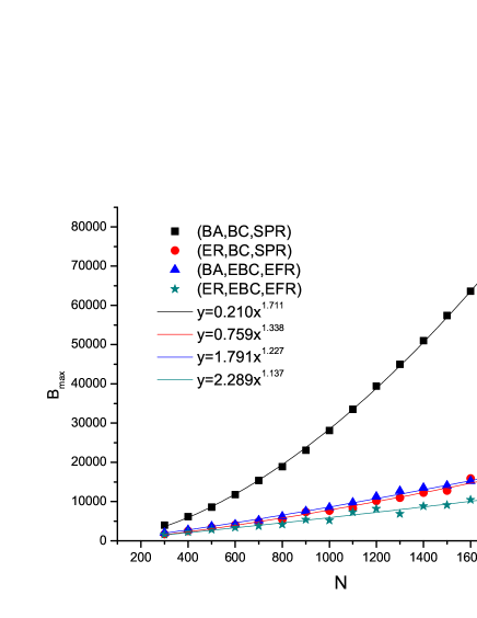
(a) $B_{max}$

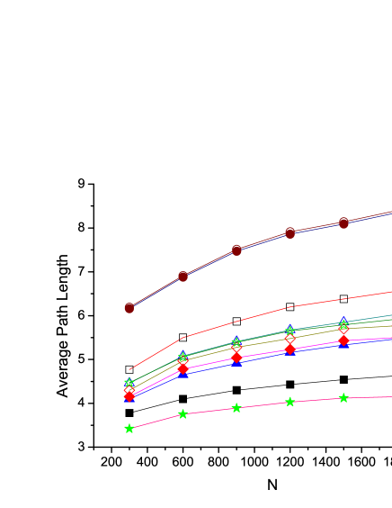
(b) APL

Figure 3: (Color online) (a) Scalability of the maximal betweenness and effective betweenness for BA and ER networks. With SPR, the $Y$-axis denotes the value of maximal betweenness, and with EFR, the $Y$-axis denotes the maximal effective betweenness. The line fittings for these data are also presented, and (b) average path length for the five networks with different size under both shortest path routing and efficient routing. The filled shape represents the SPR, while the hollow shape represents the EFR.

In most networks, $L^{(EFR)}$ is only slightly longer than $L$ (see Fig.3(b) for the average path length of different routing algorithms in different networks), so the $R_{c}$ in (EBC,EFR) is only slightly smaller than the optimal one. However, $C_{max}$ in (BC,SPR) is $\frac{L^{(EFR)}}{L}\times\frac{B_{max}}{B^{(EFR)}_{max}}$ times larger than the $C_{max}$ in (EBC,EFR). This expresses why the cost-effectiveness of (EBC,EFR) is topology-dependent.

In HOT network, although with the same skewed degree distribution, its rigid hierarchy structure restricts the flexibility in path selection, making it insensitive to routing algorithm changes, so $B_{max}$ and $B^{(EFR)}_{max}$ show no big difference. In WS network, the near uniform degree distribution makes SPR and EFR nearly identical routing algorithms, so $B_{max}$ and $B_{max}^{(EFR)}$ also show no difference. The difference between HOT and WS is that in HOT network, $C_{max}$ is high, while, in WS, $C_{max}$ is relatively low.

Scale-free networks such as BA and PA, on the other hand, have the inherent flexibility in path selection and show strong sensitivity to routing algorithm changes. In these networks, $B_{max}$ can be an order of magnitude larger than $B^{(EFR)}_{max}$, which makes $C_{max}$ in (EBC,EFR) quite smaller compared with (BC,SPR).

ER network’s random structure makes it lies somewhere between the WS and BA network. For ER network, both (BC,SPR) and (EBC,EFR) are good designing choices. Even (UC,SPR) and (UC,EFR) also achieves relatively high $R_{c}$ values compared with other networks.

VI Scalability of network designing schemes

The scalability is investigated by the growth trends of $R_{c}$ and $C_{max}$ when network evolves. Conceptually, the scalability can be viewed as a third dimension of the designing objective, i.e., the time dimension. Figure 2(a) presents the $R_{c}$ values for BA and ER networks under four different settings and Figure 2(b) presents the $C_{max}$ values for the five networks under (BC, SPR) and (EBC, EFR). It is shown that under (UC, SPR), BA network’s $R_{c}$ value remains quite stable, i.e., almost not scaling with $N$. This is because, $B_{max}$ scales super linearly with $N$, as illustrated in Fig. 3(a). Numerical fitting on simulation result shows that $B_{max}\sim N^{1.711}$ in BA network, whereas in ER network, $B_{max}\sim N^{1.338}$. On the other hand, $B^{(EFR)}_{max}$ grows much slowly as network expands, $\sim N^{1.227}$ and $\sim N^{1.137}$ for BA and ER respectively. This means with (UC, SPR), BA network’s $R_{c}$ scales very slowly, while ER network’s $R_{c}$ scales much better. However, with (UC, EFR) the scalability of $R_{c}$ significantly improves for BA network.

Regarding $C_{max}$, with (BC, SPR), $C_{max}\propto B_{max}$, so it grows fast for BA, HOT and PA networks, and much more slowly for ER and WS networks. With (EBC, EFR), $C_{max}\propto B^{(EFR)}_{max}$, which scales much slowly in BA and PA networks, but still grows fast in HOT network. This is evidenced in Fig.2(b), where $C_{max}$ grows fast with (BA, BC, SPR), (PA, BC, SPR) and (HOT, BC, SPR) and (HOT, EBC, EFR), but remains nearly stable for other settings.

In short, the above analysis show that (BC,SPR) is not a scalable designing for heterogenous networks. On the other hand, our proposed (EBC, EFR) is a cost-effective designing that is scalable for most of the networks with small-world properties, except for heterogenous networks with rigid hierarchy structure, and ER network shows the potential of achieving scalable cost-effective designing under any settings.

VII Conclusions

By proposing that network designing is not a single objective optimization process, but rather a multi-objective optimization process, this paper established a scientific foundation for network designing studies. It has been found that typical network designing objectives such as network transmission capacity and technical feasibility are often contradictive, which indicates the presence of a tradeoff issue. We defined a two dimensional cartesian system to evaluate the effect of each designing scheme.

In particular, the empirical network designing approach widely adopted today is incapable to meet the cost-effective and scalable requirements. The existence of cost-effective design depends heavily on the network topology. For BA-like scale-free networks, efficient routing combined with effective betweenness based link bandwidth allocation scheme can be regarded as a cost-effective design, and this property also scales as network evolves. If the designer has the full freedom of choosing all designing ingredients, then ER network shows pretty good characteristic in achieving a cost-effective design under most settings.

We believe the scientific framework as well as the specific findings will give insightful help to advance the science of network designing and engineering. Evaluating the performance of other designing schemes under this framework, and finding the exact boundary of the achievable area, for example, whether the boundary is concave or convex for different networks, are the direction for future work.

References

- [1] C. Wittbrodi, B. Woodcock, A. Ahuja, T. Li, V. Gill and E. Chen, ”Global routing system scaling issues”, NANOG Panel, http://www.nanog.org/mtg-0102/witt.html (2001).
- [2] G. Huston, ”Analyzing the Internet’s BGP routing table”, The Internet Protocol Journal, 4 (2001).
- [3] G. Huston ”Scaling inter-domain routing-a view forward”, The Internet Protocol Journal, 4 (2001).
- [4] A. Broido, E. Nemeth and K. Claffy, ”Internet expansion, refinement, and churn”, European Transactions on Telecommunications, 13, 33-51 (2002).
- [5] M. Faloutsos, P. Faloutsos, and C. Faloutsos, ”On power-law relationships of the Internet topology”, Proc. ACM SIGCOMM 1999 (1999).
- [6] A. L. Barabsi and R. Albert, ”Emergence of scaling in random networks”,Science 286, 509 (1999).
- [7] T. Bu and D. Towsley, ”On distinguishing between Internet power-law topology generators”, Proc. IEEE INFOCOM 2002 (2002).
- [8] S. Zhou, G. Q. Zhang, and G. Q. Zhang, “Chinese Internet AS-Level Topology,” IET Commun., 1, 209–214 (2007).
- [9] P. Mahadevan, D. Krioukov, K. Fall and A. Vahdat, ”Systematic topology analysis and generation using degree correlations”, Proc. ACM SIGCOMM 2006 (2006).
- [10] G. Q. Zhang, G. Q. Zhang, Q. F. Yang, S. Q. Cheng, and T. Zhou, ”Evolution of the Internet and its cores”, New. J. Phys. 10, 123027 (2008).
- [11] Network Seicen and Engineering(NetSE) Research Agenda, http://www.cra.org/ccc/docs/NetSE-Research-Agenda.pdf
- [12] N. Gupte and B. K. Singh, ”Role of connectivity in congestion and decongestion in networks”, Euro. Phys. B. 50, 227 (2006).
- [13] N. Gupte, B. K. Singh and T. M. Janaki, ”Networks: structure, function and optimization”, Phys. A. 346, 75 (2005).
- [14] G. Q. Zhang, S. Zhou, G. Yan, D. Wang, and G. Q. Zhang, ”Enhancing the network transmission capability by efficiently allocating node capability”, arXiv:0910.2285 (2009).
- [15] G. Q. Zhang, ”On cost-effective communication network designing”, arxiv:0910.2104 (2009).
- [16] S. P. Borgatti, ”Centrality and Network flow”, Soc. Netw. 27, 55 (2005).
- [17] K. -I. Goh, B. Kahng, and D. Kim, ”Universal behavior of load distribution in scale-free newtorks”, Phys. Rev. Lett. 87, 278701 (2001).
- [18] R. Guimer, A. Z. Guilera, F. V. Redondo, A. Cabrales, and A. Arenas, ”optimal network topologies for local search with congestion”, Phys. Rev. Lett. 89, 328170 (2002).
- [19] H. Li and M. Maresca, ”Polymorphic-torus network”, IEEE. Trans. Computers 38, 1345 (1989).
- [20] G. Q. Zhang, D. Wang, and G. J. Li, ”Enhancing the transmission efficiency by edge deletion in scale-free networks”, Phys. Rev. E 71, 017101 (2007).
- [21] G. Yan, T. Zhou, B. Hu, Z. Q. Fu, and B. H. Wang, ”Efficient routing on complex networks”, Phys. Rev. E 73, 046108 (2006).
- [22] L. Zhao, Y. C. Lai, K. Park, and N. Ye, ”Onset of traffic congestion in complex networks”, Phys. Rev. E 71, 026125 (2005).
- [23] M. E. J. Newman, ”Assortative mixing in networks”, Phys. Rev. Lett. 89, 208701 (2002).
- [24] S. N. Dorogovtsev, ”Clustering of correlated networks”, Phys. Rev. E. 69, 027014 (2004).
- [25] Archipelago Measurement Infrasture, http://www.caida.org /projects/ark/
- [26] Y. Shavtt and E. Shir, ”DIMES-letting the Internet measure itself”, http://www.arxiv.org/abs/cs.NI/0506099 (2005).
- [27] N. Spring, R. Mahajan, D. Wetherall and T. Anderson, ”Measuring ISP topologies with rocketfuel”, Proc. IEEE INFOCOM 2001 (2001).
- [28] B. Danila, Y. Yu, J. A. Marsh, and K. E. Bassler, ”Optimal transport on complex networks”, Phys. Rev. E 74, 046106 (2006).
- [29] L. Li, D. Alderson, W. Willinger, J. Doyle, ”A first principles approach to understanding the Internet’s rouer-level topology”, Proc. ACM SIGCOMM 2004 (2004).
- [30] S. Zhou and R. J. Mondragón, ”The rich-club phenomenon in the Internet topology”, IEEE Commun. Lett. 8, 180 (2004).
- [31] A. Arenas, A. Díaz-Guilera, and R. Guimerà, ”Communication in networks with hierarchical branching”, Phys. Rev. Lett. 86, 3196 (2001).
- [32] L. C. Freeman, ”Centrality in social networks: conceptual clarification”, Soc. Netw. 1, 215 (1979).
- [33] P. Erdös and A. Rényi, ”On random graphs”, Publ. Math. Debrecen 6, 290 (1959).
- [34] D. J. Watts and S. H. Strogatz, ”Collective Dynamics of small world networks”, Nature 393, 440 (1998).