Regular spiking in asymmetrically delay-coupled FitzHugh-Nagumo systems

Abstract

We study two delay-coupled FitzHugh-Nagumo systems, introducing a mismatch between the delay times, as the simplest representation of interacting neurons. We demonstrate that the presence of delays can cause periodic oscillations which coexist with a stable fixed point. Periodic solutions observed are of two types, which we refer to as a “long” and a “short” cycle, respectively.

1 Introduction

Being an inherent feature of a human, laziness was always that force which engendered invention of new devices, supposed to work instead of people. And in our epoch of vast technological progress, there are thousands of useful gadgets already existing. Though recently the science is advancing with seven-league strides, there are still a great number of phenomena which are waiting for a better insight. One has to admit that none of the existing complex machines and powerful computers can substitute a single human brain. Which means that we still do not draw close enough to clearing up a mystery of how this accumulation of grey matter really works.

Since the end of the last century, study of neural networks picks up speed. In order to describe its intricate behavior, the brain is often represented as an ensemble of coupled nonlinear dynamical elements, capable of producing spikes and exchanging information between each other [1, 2, 3]. Such neural populations are usually spatially localized and contain both excitatory and inhibitory neurons [4].

Some researchers, starting from the simplest case of two interconnected neurons, show how more complicated dynamics emerges in larger sets [5]. The others explore extremely complex network of subnetworks, focusing on the hierarchically clustered organization of interacting excitable elements [6].

Most studies base on the present oscillatory behavior of individual system elements, which then produces observable patterns due to collective synchronization [7, 8, 9]. Thus, for modeling a single neuron, phase oscillators are often used. For instance, to characterize mutual dynamics of cells in certain brain areas, responsible for giving the onset to Parkinson’s disease or epilepsy, a well-known Kuramoto model is considered [10, 11, 12, 13].

Here, we rely on the works by FitzHugh [14] and Nagumo et al.[15] who have shown that for describing the main characteristics of a neuron dynamics, it is sufficient to consider a 2-dimensional system. The latter is also widely used nowadays as one of the simplest models for examining brain dynamics and has been essentially studied in many papers (see, for instance, [16, 18, 17, 19] and references therein).

Having an intention to move from simple to complex, we consider below a set of equations consisting only of two identical FitzHugh-Nagumo subsystems (see also [20, 21]). Their interaction is described by a linear coupling term which includes delays ($\tau_{1}$ and $\tau_{2}$), accounted for the fact that the signal transmission between neurons is not instantaneous:

$$\begin{split}\epsilon\dot{x}_{1}&=x_{1}-\frac{x_{1}^{3}}{3}-y_{1}+C(x_{2}(t-\tau_{2})-x_{1}(t))\\ \dot{y}_{1}&=x_{1}+a\\ \epsilon\dot{x}_{2}&=x_{2}-\frac{x_{2}^{3}}{3}-y_{2}+C(x_{1}(t-\tau_{1})-x_{2}(t))\\ \dot{y}_{2}&=x_{2}+a\end{split}$$ (1)

Here $(x_{1},y_{1})$ and $(x_{2},y_{2})$ are the phase coordinates for the first and the second subsystem respectively. The parameter $a$ determines whether the individual neuron is in the excitable regime or exhibits self-sustained periodic firing. The time scale parameter $\epsilon$ is chosen during the numerical simulations to be $0.01$, which results in fast activator variables $x_{1}$, $x_{2}$ and slow inhibitor variables $y_{1}$, $y_{2}$. For further simplicity, the coupling strength $C$ is also taken symmetric.

2 Sketch dynamics

2.1 Fixed point

As it was already mentioned, the dynamics of an isolated 2-dimensional FitzHugh-Nagumo system is already well-investigated. Its single fixed point $P_{2}=(-a,a^{3}/3-a)$ is stable for $a>1$ and exhibits a supercritical Hopf bifurcation when the excitability parameter crosses unity, which implies periodic spiking for $a<1$. Provided that $a>1$, the system is excitable, namely, if a sufficient external impulse is added, it emits a spike and then rests again in the $P_{2}$ state.

For our numerical simulations, we take $a=1.3$, so that the individual subsystems are in the excitable regime. The coupling term of the considered form is canceled for a fixed point orbit, thus, the 4-dimensional equilibrium $P_{4}=(-a,-a+{a^{3}}/{3},-a,-a+{a^{3}}/{3})$, being existent for the uncoupled system, persists as well for the Eq. (1). Changing the coupling strength or the delays also does not influence its stability, as it was recently shown [20].

2.2 Regular spiking

However, besides the stable fixed point solution, the system (1) can also produce periodic oscillations. Intuitively, this phenomenon can be explained as follows. One can perturb, for instance, the first neuron, so that it emits a spike. Then, with the delay $\tau_{1}$ this perturbation reaches the second neuron, which provokes it to spike as well. Again with the delay $\tau_{2}$ the second neuron “informs” the first one that it has been stimulated, which causes a new run of the cycle, and the process repeats (see schematic representation in the Fig 1(a)).

Figure 1: Schematic representation of periodic firing in a system with delay. (a) “long” cycle; (b) “short” cycle

Though, in the numerical simulations, starting from various initial conditions, we observed periodic solutions of two different types, which are referred to in the following as a “long” and a “short” cycle respectively. The former is of the period $T\gtrapprox\tau_{1}+\tau_{2}$, while the latter has the period $T\gtrapprox(\tau_{1}+\tau_{2})/2$.

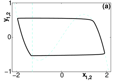
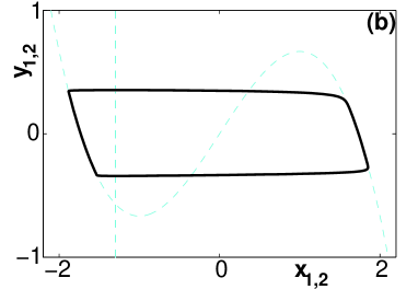
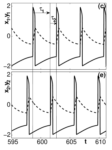
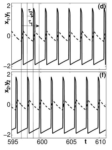
Figure 2: Phase portraits ((a) and (b)) and time series ((c), (e) and (d), (f)) for long and short cycles respectively. On the time series plots, solid line correspond to $x_{1,2}$ and dashed line correspond to $y_{1,2}$. The parameters are $a=1.3,\epsilon_{1,2}=0.01,C=0.5,\tau_{1}=3,\tau_{2}=1$.

Again, intuitively, to obtain this second solution one would add an initial impulse not to one, but to both neurons, then roughly the short cycle dynamics can be plotted as in the Fig. 1(b). One could remark that, in this case, the initial perturbation for the second neuron should arrive before the delayed signal of the first one, namely for $t\in(0,\tau_{1})$. Although there are infinitely many variations for choosing the time moment for the second impulse, in our numerical simulations we were able to observe only that pattern, which is depicted in the Fig. 1(b).

In the Fig. 2, we plot the phase portraits and the data series for these two attractors for certain fixed parameter values.

3 Periodic solutions: deeper insight

The next point to investigate in connection with the periodic firing patterns obtained, is a question whether these solutions exist for all couplings. Is their stability region large enough or such solutions appear only for separate parameter values?

3.1 “Long” cycle

As it was already noticed in [20], such oscillations appear through a saddle-node bifurcation of limit cycles, creating a pair of a stable and an unstable periodic orbit. In the Fig. 3(a), the bifurcation curves of this attractor type are plotted in the $(C,\tau_{1})$-plane, for $\tau_{2}=0.5$, $\tau_{2}=1$ and $\tau_{2}=2$. It is easy to conclude, that with increasing $\tau_{2}$ the bifurcation curve moves to the left, closer to the wall value $C=0$.

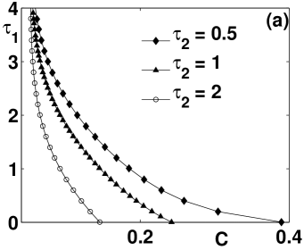
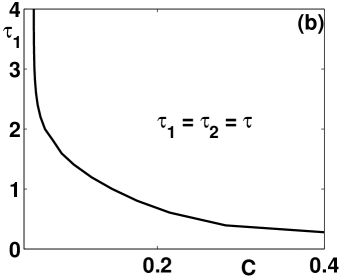
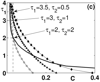
Figure 3: Bifurcation curves for appearance of the $(\tau_{1}+\tau_{2})$-periodic solution (long cycle) in $(C,\tau_{1})$-plane. (a) Diagrams for different $\tau_{2}$ values. (b) Diagram for the case of $\tau_{1}=\tau_{2}=\tau$. (c) Overlay of the figures (a) and (b). Vertical dashed line indicates a critical value of $C$.

This implies that for some large enough coupling periodic firing still exists even if one of the delays is close to zero. For comparison, in the Fig. 3(b), the bifurcation curve for the case $\tau_{1}=\tau_{2}$ is present. When overlaying the two graphs of (a) and (b) (Fig. 3(c)), one can notice that the critical coupling value (indicated by a vertical dashed line) does not depend on the delay times difference, but only on their sum (see Appendix).

In support to this last statement, we depict in the Fig. 4(a, b) phase portraits and time series for three different periodic solutions, namely $\tau_{1}=\tau_{2}=2$, $\tau_{1}=3,\tau_{2}=1$ and $\tau_{1}=3.5,\tau_{2}=0.5$, while the sum of delays is always 4 and the coupling strength $C=0.5$. As it could be clearly seen, the phase trajectories coincide perfectly as well as the time series.

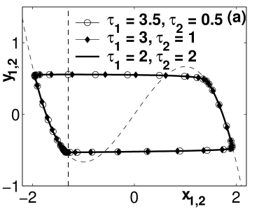
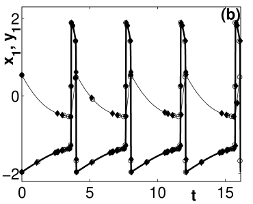
Figure 4: Phase portrait and time series for 3 different long cycles with $C=0.5$.

We also would like to examine the question how the cycle period is related to the coupling terms. The Fig. 5(a) represents several plots of the orbit period $T$ vs. $\tau_{1}$, while $\tau_{2}=0.5,1,2$ and $C=0.5$.

In the Fig. 5(b), dependence of the period on $C$ is depicted ($\tau_{2}$ is the same as in (a), and $\tau_{1}$ is chosen so that the sum of delays does not change). As it is expected (cf. [20]), $T$ increases linearly with $\tau_{1}$. However, it decays with increasing $C$.

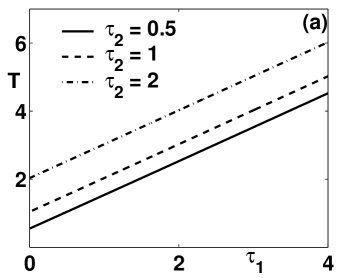
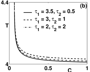
Figure 5: Evolution of the period for the long cycle solution depending on the coupling term. (a) Period $T$ vs. $\tau_{1}$ for different fixed values of $\tau_{2}$, $C=0.5$. (b) Period $T$ vs. $C$, for different values of $\tau_{1}$ and $\tau_{2}$ so that $\tau_{1}+\tau_{2}=4$.

3.2 “Short” cycle

For the short cycle, the situation is almost the same. Again it is born through a saddle-node bifurcation.

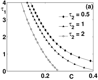
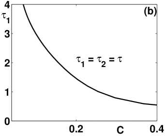
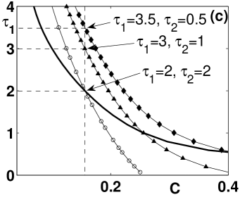
Figure 6: Bifurcation curves for appearance of the $(\tau_{1}+\tau_{2})/2$-periodic solution (short cycle) in $(C,\tau_{1})$-plane. (a) Diagrams for different $\tau_{2}$ values. (b) Diagram for the case of $\tau_{1}=\tau_{2}=\tau$. (c) Overlay of the figures (a) and (b).

In the Fig. 6(a), we also plot the bifurcation curves, separating the regions of existence and absence of the short cycle, in the $(C,\tau_{1})$-plane (as earlier $\tau_{2}=0.5$, $\tau_{2}=1$ and $\tau_{2}=2$). Again with increasing $\tau_{2}$ the bifurcation curve moves to the left, however, in comparison with the long cycle the short one occurs for larger values of coupling strength. And after laying over the curve for the case of equal delays $\tau_{1}=\tau_{2}$ (Fig. 6(b)), one can notice that the critical $C$ depends only on the delays sum (see Fig. 6(c)). The phase portraits and the time series for three different periodic solutions, plotted in the Fig. 7, coincide as well.

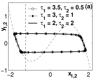
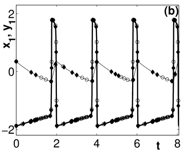
Figure 7: Phase portrait and time series for 3 different short cycles with $C=0.5$.

Finally, in the Fig. 8(a),(b), the graphs disclosing the relation between the period and the coupling term configuration are presented. As in the case of the long cycle, $T$ is a linear function of $\tau_{1}$ and has a gradual decrease on $C$.

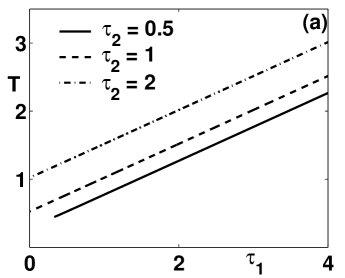
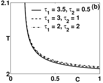
Figure 8: Evolution of the period for the short cycle solution depending on the coupling term. (a) Period $T$ vs. $\tau_{1}$ for different fixed values of $\tau_{2}$, $C=0.5$. (b) Period $T$ vs. $C$, for different values of $\tau_{1}$ and $\tau_{2}$ so that $\tau_{1}+\tau_{2}=4$.

4 Conclusions

In the present paper we have considered two asymmetrically delay-coupled FitzHugh-Nagumo systems for modelling interacting excitable neural elements. Such an “intrusion” gives rise to the regular spiking in the system investigated. For sufficiently large coupling strength and delays, one can observe periodic solutions of two different types (long and short cycles), depending on whether only one subsystem is perturbed initially or both. The long cycle period approximately equals $\tau_{1}+\tau_{2}$, while the short one has a period of about a half of this amount.

Furthermore, the numerical simulation, as well as the mathematical anlysis, shows that phase portraits and time series of these solutions do not depend on the difference of delays, but only on their sum.

5 Acknowledgements

Support from DFG in the framework of Sfb 555 is acknowledged.

The authors would like to thank G. Hiller, P. Hövel and V. Zykov for fruitful discussions and remarks.

Appendix A Transformation to symmetric coupling

Consider the general system

$$\dot{x}_{1}=f(x_{1})+C(x_{2}(t-\tau_{2})-x_{1}(t)),$$ (2)

$$\dot{x}_{2}=f(x_{2})+C(x_{1}(t-\tau_{1})-x_{2}(t)).$$ (3)

Without losing generality assume that $\tau_{1}>\tau_{2}$ and denote $\tau\equiv(\tau_{1}+\tau_{2})/2$ and $\Delta\tau\equiv(\tau_{1}-\tau_{2})/2$, so that $\tau_{1}=\tau+\Delta\tau$ and $\tau_{2}=\tau-\Delta\tau$. Then introducing a new function $\tilde{x}_{2}(t)=x_{2}(t+\Delta\tau)$ we use

$$x_{2}(t-\tau_{2})=\tilde{x}_{2}(t-\tau)$$

in eq. (2) and rewrite the equation (3) as follows

$$\begin{split}\dot{\tilde{x}}_{2}(t)&=f(\tilde{x}_{2}(t))+C(x_{1}(t+\Delta\tau-\tau_{1})-\tilde{x}_{2}(t))\\ &=f(\tilde{x}_{2}(t))+C(x_{1}(t-\tau)-\tilde{x}_{2}(t)),\end{split}$$

which leads to

$$\begin{split}\dot{x}_{1}&=f(x_{1})+C(\tilde{x}_{2}(t-\tau)-x_{1}(t)),\\ \dot{\tilde{x}}_{2}&=f(\tilde{x}_{2})+C(x_{1}(t-\tau)-\tilde{x}_{2}(t)).\end{split}$$ (4)

This corresponds to a system with symmetric delay coupling, and the function $\tilde{x}_{2}(t)$ fully coincides with the function $x_{2}(t)$ of the initial problem, but with a shift along the time axis by $\Delta\tau=(\tau_{1}-\tau_{2})/2$.

We also note that the inhibitor variables $y_{1}$, $y_{2}$ of the system (1) depend only on $x_{1}(t)$ and $x_{2}(t)$, respectively. Therefore, omitting them in the above analysis does not influence the resulting conclusion.

References

- [1] H. Haken. Brain Dynamics: Synchronization and Activity Patterns in Pulse-Coupled Neural Nets with Delays and Noise (Springer Verlag GmbH, Berlin, 2006).
- [2] H. R. Wilson. Spikes, Decisions, and Actions: The Dynamical Foundations of Neuroscience (Oxford University Press, Oxford, 1999).
- [3] W. Gerstner and W. Kistler. Spiking Neuron Models (Cambridge University Press, Cambridge, 2002).
- [4] H. R. Wilson and J. D. Cowan. Excitatory and inhibitory interactions in localized populations of model neurons. Biophysical journal 12, pp. 1–24 (1972).
- [5] A. Destexhe, D. Contreras, T. J. Sejnowski, and M. Steriade. A model of spindle rhythmicity in the isolated thalamic reticular nucleus, J. Neurophysiol. 72, pp. 803–818 (1994).
- [6] C. Zhou, L. Zemanova, G. Zamora, C. C. Hilgetag, and J. Kurths. Hierarchical organization unveiled by functional connectivity in complex brain networks, Phys. Rev. Lett. 97, p. 238103 (2006).
- [7] M. G. Rosenblum and A. Pikovsky. Controlling synchronization in an ensemble of globally coupled oscillators, Phys. Rev. Lett. 92, p. 114102 (2004).
- [8] O. V. Popovych, C. Hauptmann, and P. A. Tass. Effective desynchronization by nonlinear delayed feedback, Phys. Rev. Lett. 94, p. 164102 (2005).
- [9] M. Gassel, E. Glatt, and F. Kaiser. Time-delayed feedback in a net of neural elements: Transitions from oscillatory to excitable dynamics, Fluct. Noise Lett. 7, pp. L225–L229 (2007).
- [10] O. V. Popovych, Y. L. Maistrenko, and P. A. Tass. Phase chaos in coupled oscillators, Phys. Rev. E 71, p. 065201(R) (2005).
- [11] P. Ashwin, O. Burylko, Y. Maistrenko, and O. Popovych. Extreme sensitivity to detuning for globally coupled phase oscillators, Phys. Rev. Lett. 96, p. 054102 (2006).
- [12] Y. L. Maistrenko, B. Lysyansky, C. Hauptmann, O. Burylko, and P. A. Tass. Multistability in the Kuramoto model with synaptic plasticity, Phys. Rev. E 75, p. 066207 (2007).
- [13] P. Ashwin,O. Burylko, Y. Maistrenko. Bifurcation to heteroclinic cycles and sensitivity in three and four coupled phase oscillators, Physica D 237, pp. 454–-466 (2008).
- [14] R. FitzHugh. Impulses and physiological states in theoretical models of nerve membrane, Biophys. J. 1, pp. 445–466 (1961).
- [15] J. Nagumo, S. Arimoto, and S. Yoshizawa. An active pulse transmission line simulating nerve axon., Proc. IRE 50, pp. 2061–2070 (1962).
- [16] N. Buric and D. Todorovic. Dynamics of fitzhughnagumo excitable systems with delayed coupling, Phys. Rev. E 67, p. 066222 (2003).
- [17] R. Toral, C. Masoller, C. R. Mirasso, M. Ciszak, O. Calvo. Characterization of the anticipated synchronization regime in the coupled FitzHugh–Nagumo model for neurons, Physica A 325, pp. 192–198 (2003).
- [18] B. Lindner, J. García-Ojalvo, A. Neiman, and L. Schimansky-Geier. Effects of noise in excitable systems, Phys. Rep. 392, pp. 321–424 (2004).
- [19] H. Kitajima and J. Kurths. Synchronized firing of FitzHugh–Nagumo neurons by noise, Chaos 15, p. 023704 (2005).
- [20] M. A. Dahlem, G. Hiller, A. Panchuk, and E. Schöll. Dynamics of delay-coupled excitable neural systems, Int. J. Bif. Chaos 19, pp. 1–9 (2009).
- [21] E. Schöll, G. Hiller, P. Hövel, and M. A. Dahlem. Time-delayed feedback in neurosystems, Phil. Trans. R. Soc. A 367, pp. 1079–1096 (2009).