Clustering Phase Transitions and Hysteresis: Pitfalls in Constructing Network Ensembles

Abstract

Ensembles of networks are used as null models in many applications. However, simple null models often show much less clustering than their real-world counterparts. In this paper, we study a model where clustering is enhanced by means of a fugacity term as in the Strauss (or “triangle”) model, but where the degree sequence is strictly preserved – thus maintaining the quenched heterogeneity of nodes found in the original degree sequence. Similar models had been proposed previously in [R. Milo et al., Science 298, 824 (2002)]. We find that our model exhibits phase transitions as the fugacity is changed. For regular graphs (identical degrees for all nodes) with degree $k>2$ we find a single first order transition. For all non-regular networks that we studied (including Erdös - Rényi and scale-free networks) we find multiple jumps resembling first order transitions, together with strong hysteresis. The latter transitions are driven by the sudden emergence of “cluster cores”: groups of highly interconnected nodes with higher than average degrees. To study these cluster cores visually, we introduce q-clique adjacency plots. We find that these cluster cores constitute distinct communities which emerge spontaneously from the triangle generating process. Finally, we point out that cluster cores produce pitfalls when using the present (and similar) models as null models for strongly clustered networks, due to the very strong hysteresis which effectively leads to broken ergodicity on realistic time scales.

I Introduction

Networks are an essential tool for modeling complex systems. The nodes of a network represent the components of the system and the links between nodes represent interactions between those components. Networks have been applied fruitfully to a wide variety of social Guimer et al. (2003); Newman and Park (2003), technological Broder et al. (2000), and biological Jeong et al. (2000) systems. Many network properties have been studied to discover how different functional or generative constraints on the network influence the network’s structure. In this paper we examine five properties of particular importance: the degree sequence Newman et al. (2001), which counts the number of nodes in the network with $k$ links; the clustering coefficient Newman (2003), which measures the tendency of connected triples of nodes to form triangles; the number of $q$-cliques, i.e. complete subgraphs with $q$ nodes; the assortativity Newman (2002), which measures the tendency of nodes to connect to other nodes of similar degree; and the modularity Newman and Girvan (2004), which measures the tendency of nodes in the network to form tightly interconnected communities. Their formal definitions are recalled in Sec. 2.

Models of network ensembles are of interest because they formalize and guide our expectations about real-world networks and their properties Foster et al. (2007). The most famous are the Erdös-Rényi model of random networks Erdos and Renyi (1959), and the scale-free Barabási-Albert model Barabási and Albert (1999). Comparison with an a priori realistic “null” model can also indicate which features of a real network are expected based on the null model features, and which are surprising and thus of interest, as in motif search Milo et al. (2002). In the latter context, the most popular ensemble is the configuration model Molloy and Reed (1995) and related variants Maslov and Sneppen (2002), in which all networks with a given number of nodes and a given degree sequence have the same weight. One problem of the configuration model is that it shows far too little clustering; this problem is especially important when the model is applied to motif search in, e.g., protein interaction networks Baskerville et al. (2007).

A model where clustering can be enhanced by means of a fugacity term in a network Hamiltonian was introduced by D. Strauss Strauss (1986) and studied in detail in Park and Newman (2005). In the Strauss model, the density of edges is also controlled by a second fugacity. Thus it is a generalization of the Erdös-Rényi model with fixed edge probability, not with fixed edge number. In the Strauss model there is a strong first order phase transition Park and Newman (2005) from a phase with weak clustering to a phase where nearly all edges condensate in a single densely connected cluster consisting of high degree nodes. This phase transition is often seen as a flaw, as it does not allow the intermediate clustering observed in most real networks .

In the present paper, we introduce and analyze the Biased Rewiring Model (BRM). As in the configuration model, we fix the exact degree sequence–accounting for quenched heterogeneity in node properties. But as in the Strauss model, we control the average number of closed triangles by a Hamiltonian Park and Newman (2004) containing a conjugate fugacity $\beta$. By fixing the degree sequence we prevent the extreme condensation of edges typical of the Strauss model, and we might a priori hope to achieve a smooth control of the clustering. Indeed, a very similar model, but with a slightly different Hamiltonian, had been proposed in Milo et al. (2002).

To our surprise we found that this is not the case, and the clustering cannot be smoothly controlled. To search for phase transitions, we plotted several characteristics (number of triangles, number of $q$-cliques with $q=4$ and 5, assortativity, and modularity) against $\beta$. In all these plots and for all non-regular graphs (i.e. graphs with a non-trivial degree distribution) we found several jumps which look like first order phase transitions (or large Barkhausen jumps in ferromagnets Young et al. (1999); Perković et al. (1995); Cizeau et al. (1997). Associated with these jumps are important hysteresis effects. Further, we found that high degree nodes play a crucial role in generating these phase transitions. It is thus not surprising that a somewhat simpler scenario holds for regular graphs (same degree $k$ for all nodes), where we found a single phase transition for all $k>2$. The only case where we found no transition at all is that of regular graphs with $k=2$. Unfortunately it is only in the last, somewhat trivial, case that we can do exact analytic calculations. In all other cases our results are based on simulations.

In Milo et al. (2002), the Hamiltonian was chosen to bias not towards a larger number of triangles, but towards a specific number. In order to achieve this reliably, one needs a fugacity which is larger than that in the BRM. In the limit of large fugacities this is similar to a model with a hard constraint. In general, statistical models with hard constraints show slower relaxation and worse ergodic behavior than models with soft constraints Newman and Barkema (1999). We expect thus that hysteresis effects might be even more pronounced in the model of Milo et al. (2002) and might render it less useful as a null model, even if the problem of phase transitions is hidden. For simplicity we shall in the following call the model of Milo et al. (2002) “triangle conserving”, although the name is not strictly correct. We find that for triangle conserving rewiring, important structures remain largely unchanged on extremely long time scales, requiring particular care when using the method. In general, phase transitions, strong hysteresis, and persistent structures of highly connected nodes together present substantial pitfalls for null-models of clustered networks.

In the next section we shall collect some basic background information, including the precise definitions of the model with unbiased rewiring and the Strauss model. The definition of the BRM and our numerical procedure is given in Sec. II.F. Our main results are found in Secs. III.A to III.C, while some results for the model with hard constraints of Milo et al. Milo et al. (2002) are presented in Sec. III.D Finally, Sec. IV contains our conclusions.

II Background

II.1 Degree sequences

The degree of a node is the number of links in which the node participates. The network’s degree sequence $\{n_{k}|\;k=0,1\ldots k_{\rm max}\}$ counts the number of nodes in the network which degree $k$. The networks studied in this paper are regular ($n_{k}=\delta_{k,k_{0}}$), Erdös-Rényi (poissonian $n_{k}$), and several real world networks with fat tails. Network properties often depend strongly on the degree sequence Newman et al. (2001). Thus real networks are often compared with null models which preserve the degree sequence.

II.2 Clustering coefficient and $q$-cliques

Three nodes are connected, if at least two of the three possible links between them exits. If all three links exist, they form a triangle. The clustering coefficient Watts and Strogatz (1998) measures the “transitivity” of relationships in the network, i.e. the probability that three connected nodes are also a triangle. Denoting the number of triangles by $n_{\Delta}$ and the degree of node $i$ by $k_{i}$, one has

$$C={3n_{\Delta}\over{1\over 2}\sum_{i=1}^{N}(k_{i}-1)k_{i}}.$$ (1)

If every relationship in the network is transitive, $C=1$; if no relationships are transitive, $C=0$. Note that the denominator of equation 1 depends only on the degree sequence, and thus $C\propto n_{\Delta}$ in any ensemble with fixed degrees.

In addition to $C$, we can also define similar higher order clustering coefficients based on $q$-cliques, i.e. on complete subgraphs with $q$ nodes, as

$$C_{q}={q\;n_{q-\rm clique}\over\sum_{i=1}^{N}{k_{i}\choose q-1}},$$ (2)

where $n_{q-\rm clique}$ is the number of $q-$cliques in the network. Notice that $C=C_{3}$. As we shall see, we can use any $C_{q}$ as an order parameter in the phase transitions discussed below.

II.3 Assortativity

The assortativity $r$ measures the tendency for nodes in the network to be linked to other nodes of a similar degree. It is defined as the Pearson correlation coefficient between the degrees of nodes which are joined by a link Newman (2002).

$$r=\frac{L\sum_{i=1}^{L}j_{i}k_{i}-[\sum_{i=1}^{L}j_{i}]^{2}}{L\sum_{i=1}^{L}j_{i}^{2}-[\sum_{i=1}^{L}j_{i}]^{2}}$$ (3)

Here $L$ is the number of links in the network and $j_{i}$ and $k_{i}$ are the degrees of nodes at each end of link $i$. Thus, if high degree nodes are linked exclusively to other high degree nodes, $r\approx 1$. If high degree nodes are exclusively linked to low degree nodes, $r\approx-1$.

II.4 Modularity

There are many methods for identifying community structure in complex networks Porter et al. (2009), each with its own strengths and drawbacks. We shall use a measure proposed by Newman and Girvan Newman and Girvan (2004) called modularity. Assume one has a given partition of the network into $k$ non-overlapping communities. Define $e_{ij}$ as the fraction of all edges which connect a node in community $i$ to a node in community $j$. Thus $a_{i}=\sum_{j}e_{ij}$ is the fraction of all links which connect to community $i$. The modularity of the partition is then defined as:

$$Q=\sum_{i}(e_{ii}-a_{i}^{2}),$$ (4)

and the modularity of the network is the maximum of $Q$ over all partitions. $Q$ measures the fraction of ‘internal’ links, versus the fraction expected for a random network with the same degree sequence. It is large when communities are largely isolated with few cross links.

The main problem in computing $Q$ for a network is the optimization over all partitions, which is usually done with some heuristics. The heuristics used in the present paper is a greedy algorithm introduced by Newman Newman (2004). We start with each node in its own community (i.e., all communities are of size 1). Joining two communities $i$ and $j$ would produce a change $\delta Q_{ij}$. All pairs $(i,j)$ are checked, and the pair with the largest $\delta Q_{ij}$ is joined. This is repeated until all $\delta Q_{ij}$ are negative, i.e. until $Q$ is locally maximal. We follow the efficient implementation of this method described by Clauset et al Clauset et al. (2004).

II.5 Exponential Network Ensembles and Network Hamiltonians

Let us assume that ${\cal G}$ is a set of graphs (e.g. the set of all graphs with fixed number $N$ of nodes, or with fixed $N$ and fixed number $L$ of links, or with fixed $N$ and fixed degree sequence, …), and $G\in{\cal G}$. Following Park and Newman (2004), a network Hamiltonian $H(G)$ is any function defined on ${\cal G}$, used to define an exponential ensemble (analogous to a canonical ensemble in statistical mechanics) by assigning a weight

$$P(G)\propto e^{-H(G)}$$ (5)

to any graph, similar to the Boltzmann-Gibbs weight.

Examples of exponential ensembles are the Erdös-Rényi model $G(N,p)$ where $H=-L\ln[p/(1-p)]$ and the Strauss model with

$$H_{\rm Strauss}=\theta L-\beta n_{\Delta}.$$ (6)

Here, $p$ (which is not to be confused with $P(G)$) is the probability that a link exists between any two nodes, while $\theta$ and $\beta$ are “fugacities” conjugate to $L$ and $n_{\Delta}$, respectively.

In the configuration model, ${\cal G}$ is the set of all graphs with a fixed degree sequence and $H=0$. Thus all graphs have the same weight. In contrast, in the “triangle conserving” biased model of Milo et al. Milo et al. (2002) ${\cal G}$ is again the set of graphs with fixed degree sequence, but

$$H_{\rm Milo}=\beta|n_{\Delta}-n_{\Delta,0}|.$$ (7)

where $n_{\Delta,0}$ is some target number of triangles, usually the number found in an empirical network. Finally, in the BRM, ${\cal G}$ is again the same but

$$H_{\rm BRM}=-\beta n_{\Delta}.$$ (8)

Thus, while large weights are given in the BRM (with $\beta>0$) to graphs with many triangles (high clustering), in the model of Milo et al. (2002) the largest weights are given to graphs with $n_{\Delta}=n_{\Delta,0}$.

II.6 Simulations: Rewiring

Simulations of these ensembles are most easily done by the Markov chain Metropolis-Hastings method Newman and Barkema (1999). This is particularly easy for models without fixed degree sequences, e.g. the Strauss model. There, new configurations are simply generated by randomly adding or removing links. This is not possible for the ensembles with fixed degree sequences, where the most natural method is rewiring Maslov and Sneppen (2002). We will first discuss the unbiased case (the configuration model), and then discuss the two biased cases $H_{\rm Milo}$ and $H_{\rm BRM}$.

II.6.1 Unbiased Rewiring

Starting from a current graph configuration $G$, a new graph $G^{\prime}$ is proposed as follows: Two links which have no node in common are chosen at random, e.g. $X$—$Y$ and $W$—$Z$. Links are then swapped randomly either to $X$—$W$ and $Y$—$Z$, or to $X$—$Z$ and $Y$—$W$. If this leads to a double link (i.e. one or both of the proposed new links is already present), the new graph $G^{\prime}$ is discarded and $G$ is kept. Otherwise, $G^{\prime}$ is accepted. It is easily seen that this conserves the degree sequence, satisfies detailed balance, and is ergodic Maslov and Sneppen (2002). Thus it leads to equidistribution among all graphs with the degree sequence of the initial graph.

Although there seem to exist no exact results on the speed of equilibration, previous experience Maslov and Sneppen (2002); Baskerville et al. (2007) suggests that the above unbiased rewiring is very fast indeed, and can be used efficiently even for large networks.

II.6.2 Biased Rewiring

For biased rewiring with a Hamiltonian $H(G)$, the proposal stage is the same, and only the acceptance step has to be modified, according to the standard Metropolis-Hastings procedure Hastings (1970); Newman and Barkema (1999): If $H(G^{\prime})\leq H(G)$, then $G^{\prime}$ is accepted (unless it has a double link, of course). Otherwise the swap is accepted only with a probability

$$p=e^{H(G)-H(G^{\prime})}$$ (9)

which is less than 1.

The detailed protocols for simulating the two biased models studied in this paper are different. For the BRM we start with the actual network $G_{0}$ whose degree sequence we want to use, and propose first $M_{0}$ unbiased swaps, with $M_{0}$ sufficiently large so that we end up in the typical region of the unbiased ensemble. After that we increase $\beta$ in small steps (typically $\delta\beta=0.002$), starting with $\beta=0$. After each step in $\beta$ we propose $M_{1}$ swaps to equilibrate approximately, and then take take at fixed $\beta$ an ensemble average (with further equilibration) by making $m$ measurements, each separated by $M_{2}$ additional proposed swaps. Thus the total number of proposed swaps at each fixed $\beta$ is $M_{1}+(m-1)M_{2}$. Typically, $M_{0}\approx 10^{6},M_{1}>10^{5},M_{2}\approx 10^{3}-10^{5}$, and $m\approx 500-10,000$.

Following the $m$ measurements we increase $\beta$ and repeat this procedure, until a preset maximal value $\beta_{\rm max}$ is reached. After that, we reverse the sign of $\delta\beta$ and continue with the same parameters $M_{1},M_{2},$ and $m$ until we reach again $\beta=0$, thereby forming a hysteresis loop. Fugacity values during the ascending part of the loop will in the following be denoted by $\beta^{+}$, those in the descending part as $\beta^{-}$. In cases where we start from a real world network with $n_{\Delta,0}$ triangles, we choose $\beta_{\rm max}$ sufficiently large so that $n_{\Delta}(\beta^{+})>n_{\Delta,0}$, i.e. the clustering covered by the hysteresis loop includes the clustering coefficient of the original network.

For the biased model of Milo et al. Milo et al. (2002) we skip the first stage (i.e., we set $M_{0}=0$), and we jump immediately to a value of $\beta$ (estimated through preliminary runs) which must be larger than the smallest $\beta^{+}$ which gave rise to $n_{\Delta,0}$ triangles in the ascending part of the loop discussed above. We first make $M_{1}$ swaps to equilibrate, and then make $m$ measurements, each separated by $M_{2}$ further swaps (an alternative protocol using multiple annealing periods will be discussed in Sec. III.4). Averages are taken only over configurations with exactly $n_{\Delta,0}$ triangles. If $\beta$ is too small, the bias will not be sufficient to keep $n_{\Delta}$ near $n_{\Delta,0}$, and $n_{\Delta}$ will drift to smaller values. Even if this is not the case and if $\beta$ is sufficiently large in principle, the algorithm will slow down if $\beta$ is near its lower limit, since then $n_{\Delta}$ will seldom hit its target value. On the other hand, if $\beta$ is too large then the algorithm resembles an algorithm with rigid constraint, which usually leads to increased relaxation times. Thus choosing an optimal $\beta$ is somewhat delicate in this model.

III Results

We explored the behavior of the BRM for three different classes of degree sequences: Fixed $k$ networks, in which every node of the network is degree $k$; Poisson degree distributions as in Erdös-Rényi networks; and typical fat-tailed distributions as in most empirical networks. Although we studied many more cases (Erdös-Rényi networks with different connectivities and sizes and several different protein-protein interaction networks), we present here only results for fixed $k$ with different $k$, for one Erdös-Rényi network, and for two empirical networks with fat-tailed degree distributions: A high energy physics collaboration network Newman (2001) and a protein-protein interaction network for yeast (S. cerevisiae) Gavin et al. (2002)). In all but fixed $k$ networks we found multiple discontinuous phase transitions, while we found a single phase transition in all fixed $k$ networks with $k>2$.

III.1 Fixed $k$ networks, analytic and simulation results

Figure 1: (color online) Average number of triangles for networks with fixed $k=3$, plotted against $\beta$. All curves are obtained by full hysteresis cycles, with $M_{1}=200000$ initial swaps after increase/decrease of $\beta$, and $M_{2}=5000$ additional swaps after each of $m=40000$ measurements at the same value of $\beta$. Hysteresis loops are seen for $N\geq 200$, but not for $\leq 100$. The straight line corresponds to the approximation Eq. (11).

III.1.1 Fixed $k$ simulations

For each $k$, the configuration with maximal $n_{\Delta}$ is a disjoint set of $(k+1)-$cliques, i.e. the graph decomposes into disjoint completely connected components of $k+1$ nodes. When $N$ is divisible by $k+1$, this gives

$$n_{\Delta}^{(k,\rm max)}={N\over k+1}{k+1\choose 3}.$$ (10)

For $k=2$, this $n_{\Delta}^{(k,\rm max)}$ is reached in a smooth way. For each $k\geq 3$, in contrast, and for sufficiently large $N$, $n_{\Delta}$ first increases proportional to $\exp(\beta)$, but then the increase accelerates and finally it jumps in a discrete step to a value very close to $n_{\Delta}^{(k,\rm max)}$. This is illustrated for $k=3$ in Fig. 1, where we plot hysteresis curves for $n_{\Delta}$ against $\beta$. From this and from similar plots for different $k$ we observe the following features:

• For small $\beta$, all curves are roughly described by

  $$n_{\Delta}\approx{(k-1)^{3}\over 6}e^{\beta}$$ (11)

  (see the straight line in Fig. 1), and this approximation seems to become exact as $N\to\infty$. Notice that this implies that $n_{\Delta}$ is independent of $N$, and the clustering coefficient is proportional to $1/N$.

• While the curves are smooth and do not show hysteresis for small $N$, they show both jumps and hysteresis above a $k-$dependent value of $N$. This is our best indication that the phenomenon is basically a first order phase transition, similar to the one in the Strauss model. Above the jump, the curves saturate (within the resolution of the plot) the bound given in Eq.(10).

• The critical values of $\beta$ increase logarithmically with $N$, although a precise determination is difficult due to the hysteresis. Notice that size dependent critical points are not very common, but there are some well known examples. Maybe the most important ones are models with long range or mean field type interactions, where the number of interaction terms increases faster than $N$. In the present case the reason for the logarithmic increase of $\beta_{c}$ is that networks with fixed $k$ become more and more sparse as $N$ increases. Thus also the density of triangles (the clustering coefficient) decreases, and in a Markov chain MC method, there are increasingly more proposed moves which destroy triangles than moves which create them. To compensate for this and make the number of accepted moves equal, $\exp(\beta_{c})$ has to increase $\propto N$.

Figure 2: Average number of triangles of fixed-$k$ degree sequence networks, with $k=2,3,5,10,$ and $16$, versus the fugacity (bias) $\beta$. Network size is $N=400$ for all curves. In these simulations $\beta$ was slowly increased, until a jump in $n_{\Delta}$ was seen (for $k\geq 3$). The straight line shows the theoretical prediction for $k=2$: $n_{\Delta}=\frac{1}{6}e^{\beta}$. The inset shows $n_{\Delta}/e^{\beta}$ for $k=2$.

In Fig. 2 we show the average number of triangles as a function of $\beta$ for fixed $k$ networks, $k=2,3,5,10,$ and $16$, with $N=400$ nodes. For each curve we used $M_{1}=4000000$ initial swaps after each increase in $\beta$, and $M_{2}=200000$ additional swaps after each of $m\geq 5000$ measurements at the same value of $\beta$. For clarity we show only values for increasing $\beta$, although there is strong hysteresis for all $k\geq 3$ and for $N=400$.

For $k=2$ there is not only no hysteresis, but there is indeed no indication of any phase transition. As seen from the inset, the data for $k=2$ are for all values of $\beta$ very well described by Eq. (11), up to the point where it reaches the bound Eq.(10). Close to that point there is a tiny bump in the curve shown in the inset, that will be explained in the next sub-sub-section.

III.1.2 $k=2$ analytic results

We now give an analytical derivation of Eq. (11) for $k=2$, and we also show that this should become exact in the limit $N\to\infty$.

In a fixed $k=2$ network, there are $N$ nodes and $N$ links all arranged in a set of disjoint simple loops. Triangles are the smallest possible loops, since self-links and double links are not allowed. For large $N$ and small $\beta$ nearly all loops are large, thus the number of loops of length $<7$ is of order $1/N$ and can be neglected for $N\to\infty$ and finite $\beta$, except that we have to allow for a small fraction of loops to have length 3, in order to achieve equilibration of the rewiring procedure.

Consider now a network of size $N$ with $n_{\Delta}$ triangles and a triangle bias $\beta$. The rewiring process will reach an equilibrium, when the probability of destroying a triangle is equal to the probability of creating a new one.

First we calculate the probabilities of randomly generating a swap which destroys a triangle. The total number of ways to choose a pair of links and perform a swap is $\cal{N}$ $=\frac{N(N-1)}{2}\times 2$, where $\frac{N(N-1)}{2}$ gives the number of distinct pairs of links and the extra factor of 2 accounts for the two possible ways of swapping the links. To destroy a triangle, one of the links must be chosen from it, and the other from a larger loop (the chance that both links are chosen from triangles, which would lead to the destruction of both, can be neglected). There are $3n_{\Delta}$ possible links in triangles to choose from, and $(N-3n_{\Delta})$ links in larger loops. Thus the probability of choosing a swap which would destroy a triangle is

$$p_{\Delta-}=\frac{3n_{\Delta}(N-3n_{\Delta})\times 2}{\cal{N}}=\frac{6n_{\Delta}}{N}\times[1+O(N^{-1})],$$ (12)

where the factor of $2$ in the numerator corresponds to the fact that both possible swaps destroy a triangle and the correction term takes also into account the neglected loops of lengths 4,5, and 6.

To add a triangle to the network, two links must be chosen from the same long loop. They must be separated by exactly two links. There are $\ell$ such pairs in a loop of length $\ell$, and thus the total number of such pairs in the network is $N$, neglecting terms of $O(1)$, corresponding to the triangles and loops shorter than $7$. This leaves us with the probability of adding a triangle

$$p_{\Delta+}=\frac{N}{\cal{N}}=N^{-1}\times[1+O(N^{-1})].$$ (13)

where there is no factor of $2$ in the numerator because only one of the two possible swaps will lead to triangle creation. Balance will be achieved when

$$p_{\Delta+}=e^{-\beta}p_{\Delta-},$$ (14)

giving

$$n_{\Delta}=\frac{e^{\beta}}{6}$$ (15)

up to correction terms of order $1/N$, which is just Eq. (11) for $k=2$.

The simple exponential behavior of $n_{\Delta}$ with $\beta$ occurs because swaps create/destroy triangles (except in the rare case of breaking up a loop of length 6) independently and one at a time. For networks with nodes of degree greater than $2$ this is still basically true when $\beta$ is small. But as $\beta$ increases, nodes cluster together more densely, allowing each link to participate in many triangles. For large values of $\beta$ these links, once formed, become difficult to remove from the network. This cooperativity – in which the presence of triangles helps other triangles to form and makes it harder for them to be removed – explains intuitively the existence of first order phase transitions for $k\geq 3$ but not for $k=2$, where the cooperative effect is not possible.

Indeed, for $n_{\Delta}$ very close to $n_{\Delta}^{(2,\rm max)}$ there is some cooperativity even for $k=2$. The configuration with $n_{\Delta}=n_{\Delta}^{(2,\rm max)}$ can be changed only by breaking up two triangles and joining their links in a loop of length 6. When $n_{\Delta}$ is close to $n_{\Delta}^{(2,\rm max)}$, link swaps which involve two triangles become increasingly prevalent. The tendency to form and destroy triangles two at a time introduces a very weak cooperativity, which is only strong enough to be effective when $n_{\Delta}^{(2,\rm max)}-n_{\Delta}=O(1)$. It is thus not enough to give rise to a phase transition, but it explains the small bump seen in the inset of Fig. 2.

III.2 Networks with non-trivial degree sequences

Network properties
Network	$N$	$\langle k\rangle$	$C$	$r$	$Q$	Comment and Ref.
ER	$800$	$5.0$	$.002$	$-.0004$	$0.196$	Erdös-Rényi
HEP	$7610$	$4.1$	$.33$	$.29$	$0.397$	scientific collab. Newman (2001)
Yeast	$1373$	$10.0$	$.58$	$.58$	$0.380$	protein binding Gavin et al. (2002)

Table 1: The number of nodes $N$, the number of links $L$, the average degree $\langle k\rangle$, the clustering coefficient $C$, and the assortativity $r$ for each of the networks discussed in Sec. III.2.

Figure 3: Average number of triangles in BRM networks with an ER degree sequence with 800 nodes and $\langle k\rangle=5$, plotted against the bias $\beta$. The lower curve corresponds to slowly increasing $\beta$, the upper to decreasing $\beta$.

Figure 4: Similar to Fig. 3, but for the HEP network (see Table 1). The dotted line indicates the number of triangles in the real network.

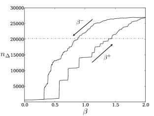
Figure 5: Similar to Fig. 3, but for the Yeast network (see Table 1).

We explored the behavior of our biased rewiring model for various degree sequences. These included Erdös-Rényi graphs with different sizes and different connectivities and several real-world networks. The latter typically show more or less fat tails. In order to find any dependence on the fatness, we also changed some of the sequences manually in order to reduce or enhance the tails. We found no significant systematic effects beyond those visible already from the following three typical networks, and restrict our discussion in the following to these: an Erdös-Rényi graph Erdos and Renyi (1959) (henceforth ER), a high energy physics collaboration network (HEP) Newman (2001), and a yeast protein binding network (Gavin et al. (2002) (Yeast). Some of their properties are collected in Table 1.

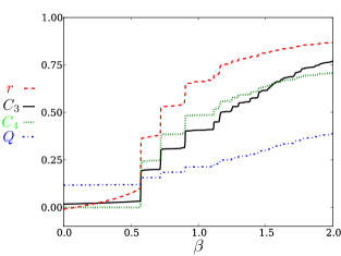
Figure 6: (color online) Four network characteristics (modularity ($Q$), clustering coefficient ($C_{3}$), 4-clique clustering coefficient ($C_{4}$), and assortativity ($r$)) for BRM networks with the Yeast degree sequence of Table 1 versus $\beta$. These data are drawn from the same simulation as in Fig. 5, but for clarity only the results for increasing values of $\beta$ are shown.

Figs. 3, 4, and 5 show $n_{\Delta}$ for these three networks. In each case $M_{0}=10^{6},M_{1}=1.5\times 10^{5},M_{2}=50000$, and $m=500$. In each of them a full hysteresis cycle is shown, with the lower curves (labeled $\beta^{+}$) corresponding to increasing and the upper curves ($\beta^{-}$) corresponding to decreasing $\beta$. In Figs. 4 and 5 the dotted line shows the number of triangles in the empirical networks.

For small values of $\beta^{+}$ all three figures exhibit a similar exponential increase in the number of triangles as that observed in fixed $k$ networks. At different values of $\beta$, however, there is a sudden, dramatic increase in $n_{\Delta}$, which does not, however, lead to saturation as it did for fixed $k$. This first phase transition is followed by a series of further transitions through which the network becomes more and more clustered. Many of them are comparable in absolute magnitude to the first jump. Although the rough positions of the jumps depend only on the degree sequences, their precise positions and heights change slightly with the random number sequences used and with the speed with which $\beta$ is increased. Thus the precise sequence of jumps has presumably no deeper significance, but their existence and general appearance seems to be a universal feature found in all cases.

Associated with the jumps in $n_{\Delta}$ are jumps in all other network characteristics we looked at, see Fig. 6. Although the locations of the jumps in $n_{\Delta}$ depend slightly on the details of the simulation, the jumps in the other characteristics occur always at exactly the same positions as those in $n_{\Delta}$. Obviously, at each jump a significant re-structuring of the network occurs, which affects all measurable quantities. Speculations how these reorganizations can be best described and what is their most “natural” driving mechanism will be given in the next subsection.

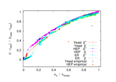
Figure 7: (color online) Values of the rescaled characteristics $n_{\Delta}/n_{\Delta,\rm max}$ and $(r-r_{\rm min})/(r_{\rm max}-r_{\rm min})$, measured at the same values of $\beta^{\pm}$, and plotted against each other. The points represent the values for the real HEP and Yeast networks.

In the downward branch of the hysteresis loop, as $\beta^{-}$ decreases toward zero, the number of triangles remains high for a long time, forming a significant hysteresis loop. This loop suggests that all jumps should be seen as discontinuous (first order) phase transitions. Since all studied systems are finite, these hysteresis loops would of course disappear for infinitely slow increase/decrease of the bias. But the sampling shown involved $>25$ million attempted swaps at each value of $\beta$, and no systematic change in the hysteresis was seen when compared to twice as fast sweeps.

In Fig. 7, we plotted $n_{\Delta}$ against the assortativity for the same values of $\beta^{\pm}$, normalizing both quantities to the unit interval. The hope was that in this way we would get universal curves which are the same for $\beta^{+}$ and $\beta^{-}$, and maybe even across different networks. Indeed we see a quite remarkable data collapse. It is certainly not perfect, but definitely better than pure chance. It suggests that biasing with the BRM leads to networks where the two characteristics $n_{\Delta}/n_{\Delta,\rm max}$ and $(r-r_{\rm min})/(r_{\rm max}-r_{\rm min})$ are strongly – but non-linearly – correlated. This indicates a potential scaling relationship between these network parameters in our model. For the two empirical networks, we show also the real values of these characteristics. They fall far from the common curve, indicating that these networks are not typical for the BRM with any value of $\beta$.

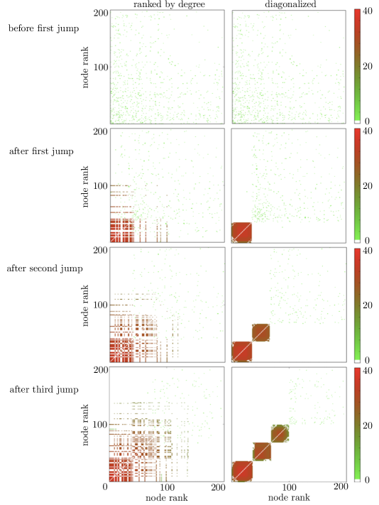
Figure 8: (color online) Relevant parts of 3-clique adjacency plots for the Yeast degree sequence. The color of each point indicates the number of $3$cliques (or triangles) in which the link participates, as given by the scale on the right hand side. Each pair of plots shows (from top to bottom) the 3CAP for a typical member of the ensemble shortly before the first jump seen in Fig. 5, shortly after it, shortly after the second jump, and shortly after the third jump. The plots on the left hand side show the 3CAP with the nodes ranked in order of their degree. In the “diagonalized” plots we rearranged the ranking so that nodes which participate in the three clusters formed by each jump are ranked together, at the head of the list. The rest of the nodes are ranked by degree.

Among the three networks studied here, the ER network is closest to a fixed $k$ network, and it should thus show behavior closest to that studied in the last subsection. This is not very evident from Figs. 3 to 5. On the other hand, we see clearly from these figures that the position of the first transition – in particular in $\beta^{+}$ – decreases with the average degree. Also, hysteresis seems to be more closely tied to individual jumps for ER, while it is more global (and thus also more important overall) for HEP and Yeast.

For the HEP and Yeast networks, we can compare the clustering of the BRM ensemble to that in the real empirical networks. The latter numbers are shown as a dashed lines in Figs. 4 and 5. In both cases, the line intersects the hysteresis loop where it is very broad. This means that a large value of $\beta^{+}$ is required to reach the real network’s level of clustering when the bias is increased, whereas a much lower value $\beta^{-}$ must be reached before these triangles can be rewired out of the network again. This gap between $\beta^{+}$ and $\beta^{-}$ at fixed $n_{\Delta}$ has important implications for the triangle “conserving” null model of Ref. Milo et al. (2002), as we will discuss later.

III.3 Clique adjacency plots and clustering cores

Up to now we have not given any intuitive arguments why clustering seems to increase in several jumps, and not in one single jump or in a continuous way. A priori one might suggest that each jump is related to the break-up of a connected component into disconnected subgraphs, just as the phase transition in regular graphs was associated to such a break-up. By counting the numbers of disconnected components we found that this is not the case, except in special cases .

Instead, we will now argue that each jump is associated with the sudden formation of a highly connected cluster of high degree nodes. The first jump in a scan with increasing $\beta$ occurs when some of the strongest hubs link among themselves, forming a highly connected cluster. Subsequent jumps indicate the formations of other clusters with high intra- but low inter-connections. What distinguishes this picture from the standard modularity observed in many real-world networks is that it automatically leads to large assortativity: Since it is high degree nodes which form the first cluster(s), there is a strong tendency that clusters contain nodes with similar degrees (for previous discussions on how clustering of nodes depends on their degree, see e.g. Ravasz and Barabási (2003); Soffer and Vázquez (2005)). Even though the modules formed are somewhat atypical, the BRM does demonstrate the ability of a bias for triangle formation to give rise to community structure de novo, whereas in other models, community structure must be put in by hand Newman and Park (2003).

In the following, the clusters of tightly connected nodes created by the BRM are called clustering cores. To visualize them, we use what we call $q$-clique adjacency plots (qCAPs) in the following. A $q$-clique adjacency plot is based on an integer-valued $N\times N$ matrix $T^{q}_{ij}$ called the $q$-clique adjacency matrix. It is defined as $T^{q}_{ij}=0$ when there is no link between $i$ and $j$, and otherwise as the number of $q$-cliques which this link is part of. In other words, if $q=3$, $T^{q=3}_{ij}$ is non-zero only when $i$ and $j$ are connected, and in the $3$CAP case it counts the number of common neighbors. $T^{q}_{ij}$ can be considered a proximity measure for nodes: linked nodes with many common neighbors are likely to belong to the same community. Similar proximity measures between nodes which depend on the similarity of their neighborhoods have been used in Ravasz et al. (2002); Leicht et al. (2006); Ahn et al. (2009). To visualize $T_{ij}$, we first rank the nodes and then plot for each pair of ranks a pixel with corresponding color or gray scale. Possible ranking schemes are by degree, by the number of triangles attached to the node, or by achieving the most simple looking, block diagonalized, $q$-clique adjacency.

Examples for the Yeast degree sequence are given in Fig. 8. The four rows, descending from the top, show the 3CAP for typical members of the BRM ensemble before the first jump and after the first, second, and third jumps. The plots in the left column show the ranking done by the degrees of the nodes. The plots on the right show the same matrices after “diagonalization”, with the nodes forming the first cluster placed in the top ranks, followed by the nodes forming the second cluster, and the nodes forming the third cluster. Only the relevant parts of the 3CAPs are shown: nodes with lower ranks do not play any substantial role except for very large values of $\beta$. We notice several features:

• Not all highest degree nodes participate in the first clustering cores. Obviously, the selection of participating nodes is to some degree random, and when sufficiently many links are established they are frozen and cannot be changed easily later. This agrees with our previous observation that the positions of the jumps change unsystematically with details like the random number sequence or the speed with which $\beta$ is increased.

• Clustering cores that have been formed once are not modified when $\beta$ is further increased. Again this indicates that existing cores are essentially frozen.

• Clustering cores corresponding to different steps do not overlap.

All three points are in perfect agreement with our previous finding that hysteresis effects are strong and that structures which have been formed once are preserved when $\beta$ is increased further.

From other examples (and from later jumps for the same Yeast sequence) we know that the last two items in the list are not strictly correct in general, although changes of cores and overlap with previous cores do not occur often. Thus the results in Fig. 8 are too extreme to be typical. When a clustering core is formed, most of the links connected to these nodes will be saturated, and the few links left over will not have a big effect on the further evolution of the core.

We find that as $\beta^{-}$ decreases, the clustering cores persist well below the value of $\beta^{+}$ at which they were created (not shown here). This shows again that once a link participates in a large number of triangles, it is very stable and unlikely to be removed again.

$3$-clique adjacency plots are also useful for analyzing empirical networks, independent of any rewiring null model, to help visualize community structure. While nodes in different communities often are linked, these links between communities usually take part in fewer triangles than links within communities. Thus simply replacing the standard adjacency matrix by the $3$clique adjacency matrix should help discover and highlight community structure Ravasz et al. (2002); Leicht et al. (2006); Ahn et al. (2009).

In the top left panel of Figs 9 and 10 we show parts of the 3CAPs for the yeast protein-protein interaction and HEP networks respectively. In both cases, nodes are ranked by degree. We see that the triangles are mostly formed between strong hubs, as we should have expected. But clustering in the real networks does not strictly follow the degree pattern, in the sense that some of the strongest hubs are not members of prominent clusters. This shows again that real networks often have features which are not encoded in their degree sequence, and that a null model entirely based on the latter will probably fail to reproduce these features. We see also that links typically participate in many triangles, if they participate in at least one. This is in contrast to a recently proposed clustering model, which assumes that each link can only participate in a single triangle Newman (2009).

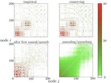
Figure 9: (color online) Parts of 3CAPs for the real yeast protein-protein interaction network of Gavin et al. (2002), for a typical network of the “triangle conserving” ensemble with no annealing, for a network obtained after an “annealing” period with $\beta=0$ and a subsequent quench with $\beta\neq 0$ using ‘triangle conserving” rewirings Milo et al. (2002), and for an ensemble obtained by 500 of such annealing/quenching alternations.

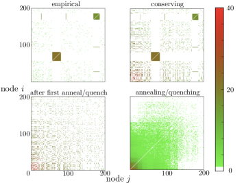
Figure 10: (color online) Analogous to Fig. 9, but for the real high energy physics collaboration network and for the HEP degree sequence, respectively.

III.4 Triangle conserving null models

In the previous subsection we considered the case where the bias is “unidirectional”. In contrast to this, Milo et al. Milo et al. (2002) considered the case where the bias tends to increase the number of triangles when it is below a number $n_{\Delta,0}$, but pushes it down when it is above. In this way one neither encounters any of the jumps discussed above nor any hysteresis. But that does not mean that the method is not plagued by the same basic problem, i.e. extreme sluggish dynamics and effectively broken ergodicity.

In the most straightforward implementation of triangle conserving rewiring with the Hamiltonian $H_{\rm Milo}$ Milo et al. (2002) one first estimates during preliminary runs a value of $\beta$ which is sufficiently large so that $n_{\Delta}$ fluctuates around $n_{\Delta,0}$. Then one starts with the original true network and rewires it using this $\beta$, without first ‘annealing’ it to $\beta=0$. The effect of this is seen in the top right panels of Figs. 9 and 10. In both cases, the $3$CAPs shown were obtained after $>10^{9}$ attempted swaps. At $\beta=0$, this number would have been much more than enough to equilibrize the ensemble. But for the large values of $\beta$ needed for these plots ($\beta=1.5$ for Yeast, and $\beta=2.4$ for HEP), few changes from the initial configurations are seen. This is particularly true for the strongest clusters existing in the real networks. Triangles not taking part in these clusters change more rapidly, but are also less important.

Thus we see a pitfall inherent in triangle conserving rewiring: when the bias is strong enough to push the number of triangles in the network up to the desired target number, the bias will also be large enough that links between high degree nodes are hardly ever randomized.

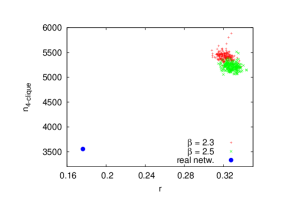
Figure 11: (color online) Values of the assortativity $r$ and of the number of 4-cliques in the real HEP network and in 400 members of the triangle-conserving biased ensemble. These 400 realizations were obtained approximately by 200 anneal/quench cycles with $\beta=2.3$ and 200 cycles with $\beta=2.5$, as described in the text. Notice that the results for biased simulations should become more exact as $\beta$ decreases towards $\beta_{c}\leq 2$.

As a way out of this dilemma, we can alternate epochs where we use triangle conserving swaps with “annealing periods” where we use $\beta=0$. In this way we would guarantee that memory is wiped out during each annealing period (see the lower left panels in Figs. 9 and 10), and each “quenching epoch” would thus contribute essentially one independent configuration to the ensemble. After many such cycles we would obtain an ensemble which looks much more evenly sampled (lower right panels in Figs. 9 and 10), although even then we can not be sure that it really represents the equilibrium ensemble for the Hamiltonian $H_{\rm Milo}$. Apart from the last caveat, the method would presumably be too slow for practical applications where high accuracy and precise variances of ensemble observables are needed, since one needs one entire cycle per data point. But it can be useful in cases where it is sufficient to estimate fluctuations roughly, and where high precision is not an issue. To illustrate this, we present in Fig. 11 results for the HEP network where we made 200 anneal/quench cycles for two different values of $\beta$ ($\beta=2.3$ and $\beta=2.5$). In each cycle the quenching was stopped when the number of triangles reached the value of the real network, and the values of $r$ and of the number of 4-cliques was recorded. We see from Fig. 11 that these values scatter considerably, but are in all cases far from the values for the real network. Thus the ensemble is a poor model for the real HEP network. We also see from Fig. 11 that $r$ and $n_{\rm 4-clique}$ depend slightly on $\beta$ (as was expected), but not so much as to invalidate the above conclusion.

IV Conclusion

In highly clustered networks – and that means for most real world networks – most of the clustering is concentrated amongst the highest degree nodes. The Strauss model correctly pointed to an important feature: clustering tends to be cooperative. Once many triangles are formed in a certain part of the network, they help in forming even more. Thus, clustering cannot be smoothly and evenly introduced into a network; it is often driven by densely interconnected, high-degree regions of the network. In triangle biased methods these high-degree regions can emerge quite suddenly and thereafter prove quite resistant to subsequent randomization.

The biased rewiring model studied in the present paper is of exponential type, similar to the Strauss model, with the density of triangles controlled by a ‘fugacity’ or inverse ‘temperature’ $\beta$. However, we prevent the catastrophic increase of connectivity at the phase transition of the Strauss model by imposing a fixed degree sequence. Yet there is still a first order transition for homogeneous networks, i.e. those with fixed degree. In the phase with strong clustering (large fugacity / low temperature), the configuration is basically a collection of disjoint $k-$cliques.

If the degree sequence is not trivial, the formation of clustering cores can no longer happen at the same $\beta$ for different parts of the network. Thus the single phase transition is replaced by a sequence of discrete and discontinuous jumps, which resemble both first order transitions and Barkhausen jumps. As in the real Barkhausen phenomenon, frozen randomness is crucial for the multiplicity of jumps. There, each jump corresponds to a flip of a spin cluster already defined by the randomness – at least at zero temperature Perković et al. (1995); Cizeau et al. (1997). In the present case, however, each jump corresponds to the creation of a cluster whose detailed properties are not fixed by the quenched randomness (the degree sequence), but depend also on the ‘thermal’ (non-quenched) noise.

As in any first order phase transition, our model shows strong hysteresis. Clustering cores, once formed, are extremely stable and cannot be broken up easily later. This limits its usefulness as a null model, even if it is treated numerically such that the phase transition jumps do not appear explicitly, as in the version of Milo et al. (2002). Because of the very slow time scales involved, Monte Carlo methods cannot sample evenly from these ensembles. Care should be taken to demonstrate that results found using them are broadly consistent across various sampling procedures.

The spontaneous emergence of clustering cores in the BRM does suggest that triangle bias can give rise to community structure in networks, without the need to define communities a priori, thanks to the cooperativity of triangle formation.

Together with jumps in the number of triangles (i.e. in the clustering coefficient), there are also jumps in all other network properties at the same control parameter positions. In particular, we found jumps in the number of $k-$cliques with $k>3$, in the modularity, and in the assortativity. This immediately raises the question whether the model can be generalized so that a different fugacity is associated to each of these quantities. For assortativity, this was proposed some time ago by Newman Newman (2002). With the present notation, biased rewiring models with and without target triangle number $n_{\Delta,0}$ and target assortativity $r_{0}$ are given by the Hamiltonians

$$H_{\rm Milo}(G;\beta,\gamma)=\beta|n_{\Delta}(G)-n_{\Delta,0}|+\gamma|r(G)-r_{0}|$$ (16)

and

$$H_{\rm BRM}(G;\beta,\gamma)=-\beta n_{\Delta}(G)-\gamma r(G),$$ (17)

respectively, where $\gamma$ is the fugacity associated to the assortativity. It is an interesting open question whether such a model might lead to less extreme clustering and thus might be more realistic. First simulations indicate that driving assortativity leads to smooth increases of all other quantities without jumps. The reason for that seems to be that the basic mechanism leading to increased assortativity – the replacement of existing links by links between similar nodes – is not cooperative, but further studies are needed.

As Newman remarked in Newman (2009), clustering in networks “has proved difficult to model mathematically.” In that paper he introduced a model where each link can participate in one triangle at most. In this way, the phase transitions seen in the Strauss model and in the present model are avoided. However, in the real-world networks studied here we found that the number of triangles in which a link participates is broadly distributed, suggesting that the Newman model Newman (2009) may not be realistic for networks with significant clustering. Indeed, specifying for each link the number of triangles in which it participates adds valuable information to the adjacency matrix (which just specifies whether the link exists or not). The resulting ‘$3$ clique adjacency plots’ revealed structures which would not have been easy to visualize otherwise and are useful also in other contexts. Thus, in contrast to what is claimed in Newman (2009), the quest for realistic models for network clustering is not yet finished.

References

- Guimer et al. (2003) R. Guimer , L. Danon, A. D az-Guilera, F. Giralt, and A. Arenas, Phys. Rev. E 68, 065103 (2003).
- Newman and Park (2003) M. E. J. Newman and J. Park, Phys. Rev. E 68, 036122 (2003).
- Broder et al. (2000) A. Broder, R. Kumar, F. Maghoul, P. Raghavan, S. Rajagopalan, R. Stata, A. Tomkins, and J. Wiener, Computer Networks 33, 309 (2000), ISSN 1389-1286.
- Jeong et al. (2000) H. Jeong, B. Tombor, R. Albert, Z. N. Oltvai, and A. Barabási, Nature 407, 651 (2000), ISSN 0028-0836.
- Newman et al. (2001) M. E. J. Newman, S. H. Strogatz, and D. J. Watts, Phys. Rev. E 64, 026118 (2001).
- Newman (2003) M. E. J. Newman, Phys. Rev. E 68, 026121 (2003).
- Newman (2002) M. E. J. Newman, Phys. Rev. Lett. 89, 208701 (2002).
- Newman and Girvan (2004) M. E. J. Newman and M. Girvan, Phys. Rev. E 69, 026113 (2004).
- Foster et al. (2007) J. G. Foster, D. V. Foster, P. Grassberger, and M. Paczuski, Phys. Rev. E 76, 046112 (2007), URL http://link.aps.org/abstract/PRE/v76/e046112.
- Erdos and Renyi (1959) P. Erdos and A. Renyi, Publ. Math. Debrecen 6, 156 (1959).
- Barabási and Albert (1999) A.-L. Barabási and R. Albert, Science 286, 509 (1999).
- Milo et al. (2002) R. Milo, S. Shen-Orr, S. Itzkovitz, N. Kashtan, D. Chklovskii, and U. Alon, Science 298, 824 (2002).
- Molloy and Reed (1995) M. Molloy and B. Reed, Comb., Prob. and Comput. 6, 161 (1995).
- Maslov and Sneppen (2002) S. Maslov and K. Sneppen, Science 296, 910 (2002).
- Baskerville et al. (2007) K. Baskerville, P. Grassberger, and M. Paczuski, Phys. Rev. E 76, 036107 (2007).
- Strauss (1986) D. Strauss, SIAM Review 28, 513 (1986), ISSN 00361445.
- Park and Newman (2005) J. Park and M. E. J. Newman, Phys. Rev. E 72, 026136 (2005).
- Park and Newman (2004) J. Park and M. E. J. Newman, Phys. Rev. E 70, 066117 (2004).
- Young et al. (1999) H. D. Young, R. A. Freedman, T. R. Sandin, and A. L. Ford, Sears and Zemansky’s University Physics, 10th ed. (Reading, MA: Addison-Wesley, 1999).
- Perković et al. (1995) O. Perković, K. Dahmen, and J. P. Sethna, Phys. Rev. Lett. 75, 4528 (1995).
- Cizeau et al. (1997) P. Cizeau, S. Zapperi, G. Durin, and H. E. Stanley, Phys. Rev. Lett. 79, 4669 (1997).
- Newman and Barkema (1999) M. E. J. Newman and G. T. Barkema, Monte Carlo methods in statistical physics (Oxford Univ. Press, 1999).
- Watts and Strogatz (1998) D. J. Watts and S. H. Strogatz, Nature 393, 440 (1998), ISSN 0028-0836.
- Porter et al. (2009) M. A. Porter, J. Onnela, and P. J. Mucha (2009), eprint arXiv:0902.3788v2.
- Newman (2004) M. E. J. Newman, Phys. Rev. E 69, 066133 (2004).
- Clauset et al. (2004) A. Clauset, M. E. J. Newman, and C. Moore, Phys. Rev. E 70, 066111 (2004).
- Hastings (1970) W. K. Hastings, Biometrika 57, 97 (1970).
- Newman (2001) M. E. J. Newman, PNASca 98, 404 (2001).
- Gavin et al. (2002) A. Gavin, M. Bosche, R. Krause, P. Grandi, M. Marzioch, A. Bauer, J. Schultz, J. M. Rick, A. Michon, C. Cruciat, et al., Nature 415, 141 (2002).
- Ravasz and Barabási (2003) E. Ravasz and A. Barabási, Phys. Rev. E 67, 026112 (2003).
- Soffer and Vázquez (2005) S. N. Soffer and A. Vázquez, Phys. Rev. E 71, 057101 (2005).
- Ravasz et al. (2002) E. Ravasz, A. L. Somera, D. A. Mongru, Z. N. Oltvai, and A.-L. Barabási, Science 297, 1551 (2002).
- Leicht et al. (2006) E. A. Leicht, P. Holme, and M. E. J. Newman, Phys. Rev. E 73, 026120 (2006).
- Ahn et al. (2009) Y.-Y. Ahn, J. P. Bagrow, and S. Lehmann (2009), eprint arXiv:0903.3178v2.
- Newman (2009) M. E. J. Newman, Phys. Rev. Lett. 103, 058701 (2009).
- Achlioptas et al. (2009) D. Achlioptas, R. D’Souza, and J. Spencer, Science 323, 1453 (2009).