Gas Accretion from a Circumbinary Disk

Abstract

A new computational scheme is developed to study gas accretion from a circumbinary disk. The scheme decomposes the gas velocity into two components one of which denotes the Keplerian rotation and the other of which does the deviation from it. This scheme enables us to solve the centrifugal balance of a gas disk against gravity with better accuracy, since the former inertia force cancels the gravity. It is applied to circumbinary disk rotating around binary of which primary and secondary has mass ratio, 1.4:0.95. The gravity is reduced artificially softened only in small circular regions around the primary and secondary. The radii are 7 % of the binary separation and much smaller than those in the previous grid based simulations. 7 Models are constructed to study dependence on the gas temperature and the initial inner radius of the disk. The gas accretion shows both fast and slow time variations while the binary is assumed to have a circular orbit. The time variation is due to oscillation of spiral arms in the circumbinary disk. The masses of primary and secondary disks increase while oscillating appreciably. The mass accretion rate tends to be higher for the primary disk although the secondary disk has a higher accretion rate in certain periods. The primary disk is perturbed intensely by the impact of gas flow so that the outer part is removed. The secondary disk is quiet in most of time on the contrary. Both the primary and secondary disks have traveling spiral waves which transfer angular momentum within them.

1 INTRODUCTION

Accretion from a circumbinary disk is expected to play an essential role in binary formation. Current star formation theory assumes that stars have only 0.01 M_⊙ at their birth and gain most of the mass at the main sequence stage through gas accretion. The accretion is mainly through disks surrounding the stars. When the stars are members of binaries, they are expected to accrete gas from the circumbinary disks when they are young.

Recent infrared imaging observations support the gas accretion from the circumbinary disk. The disk around CoKu Tauri/4 is of circumbinary rather than the transitional (Ireland & Kraus, 2008). The inner hole of the disk is likely to be cleared by the newly discovered binary with the separation of $\sim$8 AU. UY Aur has a circumbinary disk having a clumpy structure (Hioki et al., 2007), which implies dynamical interaction with the binary inside the disk.

Despite the importance, gas accretion is still mysterious in binary system. The first numerical simulation of the gas accretion onto binary was performed by Artymowicz & Lubow (1996). They demonstrated mass flow through gaps in circumbinary disks by SPH simulations. Shortly later Bate & Bonnnell (1997) demonstrated that the secondary has a much higher accretion rate than the primary when accreting gas has a relatively large angular momentum. Their result seems to be plausible since the secondary has a larger orbit and hence is closer to the inner rim of the circumbinary disk. If this is the case, however, the mass ratio should increase and approach to unity. Accordingly equal mass binaries should be dominant in contradiction to observed statistics. Unequal mass binaries are rather common. According to Duquennoy & Mayor (1991), the mean mass ratio is $\sim$ 0.4 for the solar type star stars. Reid & Gizis (1997) finds that the mass ratio distribution is approximately flat. Although the statistic may suffer from observational selection bias, unequal mass binaries are surely not rare. Present SPH simulations of star formation predict dominance of nearly equal mass binaries and do not reproduce the statistics (see, e.g., Delgad-Doanate, 2004; Clarke, 2008).

Ochi et al. (2005), which is referred as Paper I in the following, computed gas accretion onto binary using a grid based code and obtained qualitatively different results. The primary has a larger accretion rate in their simulations. Their simulations employ different methods and assumptions from those of the previous SPH simulations. First the SPH simulations are three dimensional, while Paper I is two dimensional. Second the SPH simulations assume a cold isothermal gas while Paper I assumes a warm isothermal gas. Third the method of gravity softening is different. The SPH particles are absorbed when they enter into the regions close to either of the primary and secondary. On the other hand, the gas is accumulated in the regions around the primary and secondary in Paper I. The regions of artificial gravity softening are much wider in Paper I. The radii are 5 % of the binary separation in the SPH simulations while they are 20 % of the binary separation in Paper I.

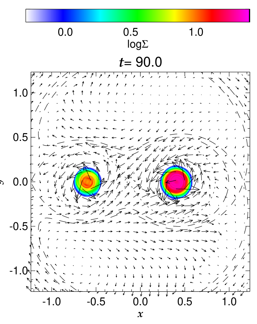
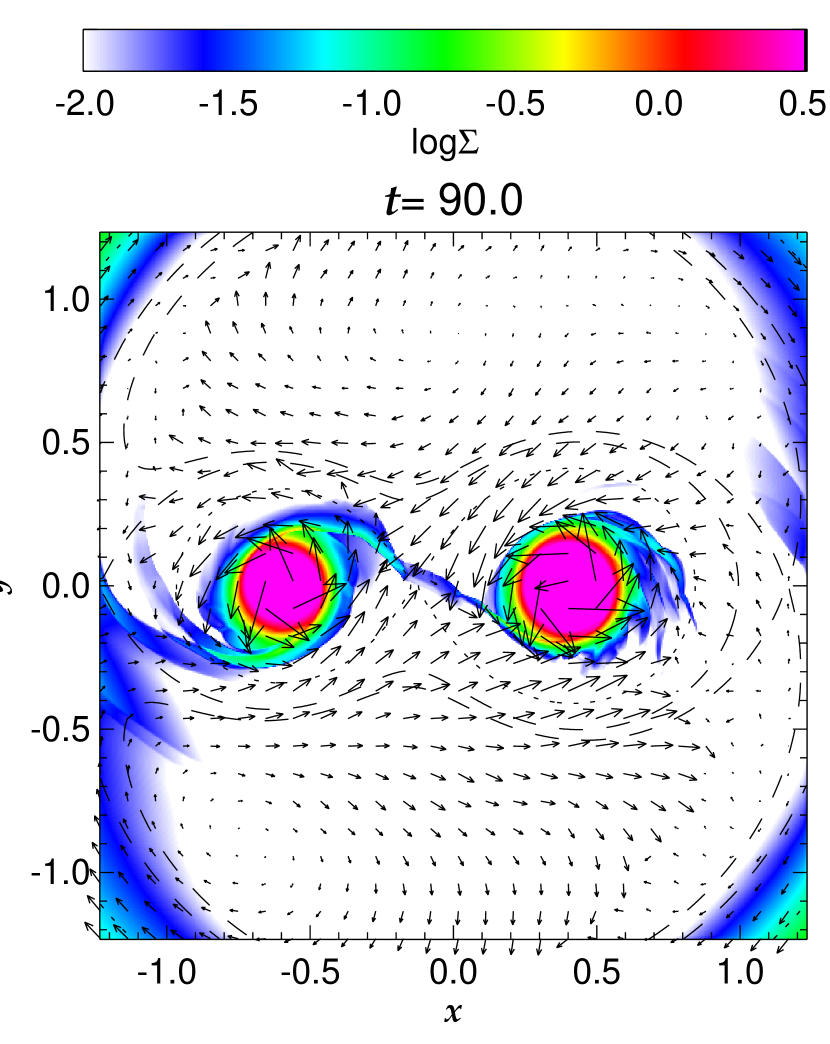
Figure 2: The surface density (color) and velocity (arrows) distributions inside the Roche lobe at $t$ = 90.0 in model 1. The dashed curves are the contours of the Roche potential. The left and right panels denote the same stage but in the different color scales.

The differences mentioned above may not account for the difference in the results (see, e.g., Clarke, 2008). The gas is concentrated on the orbital plane in the SPH simulations. Two dimensional SPH simulations assuming a warm gas does not reproduce the gross features of Paper I, as shown in Figure 2 of Clarke (2008). This discrepancy should be resolved to clarify the mystery of unequal mass binaries.

We have developed a new scheme to solve gas accretion onto binary, since an ordinary grid-based scheme does not work in practice.

A standard scheme demands a high spatial resolution around the primary and secondary so that the grid spacing is much smaller than the scaleheight. The scale height around the primary is evaluated to be $H_{1}~{}=~{}r_{1}^{2}c_{s}^{2}/(GM)$, where $r_{1}$, $c_{s}$, $G$, and $M_{1}$ denote the radial distance from the primary, the sound speed, the gravitational constant, and the primary mass, respectively. Then the required spatial resolution is expressed as $\Delta r\,\ll\,(c_{s}/v_{\varphi})^{2}r$, where $v_{\varphi}$ denotes the Keplerian rotation velocity around the primary, $\sqrt{GM_{1}/r_{1}}$. The required resolution is enormous even when the gas is relatively warm. Paper I studies the warm gas of $c_{s}\,=\,0.25$ in the unit system in which the binary separation and angular velocity are unity. When the mass ratio is $q~{}=~{}0.7$, the scaleheight is $H_{1}\,=\,0.021$ at $r_{1}\,=\,0.2$, i.e., at the outer edge of the region of artificial gravitational softening. If the gas is colder or closer to the primary, the scaleheight is shorter and higher spatial resolution is required.

We have overcome the difficulty by introducing the reference velocity. The reference velocity is set so that the acceleration cancels the gravity. The introduction of reference velocity reduces the source term in the hydrodynamical equations. As a result we have succeeded in reducing the softening radius down to 7 % of the mean separation.

The new scheme improved solutions around the primary and secondary. This improvement is essential to examine the discrepancy between the SPH simulations and Paper I. The discrepancy is prominent within the Roche lobe. The accretion from the circumbinary disk is mainly through L2 point, i.e., the side close to the secondary. The gas streams around the secondary in Paper I while it accretes onto the secondary in SPH simulations. Although shock waves form in both types of simulations, the location is scheme dependent. The recipient of gas accretion depends critically on the shock location, since the shock energy dissipation settles the gas. The flow is highly supersonic in the circumstellar disks, since the Keplerian rotation velocity is $v_{\varphi}~{}=~{}1.71~{}(r_{1}/0.2)^{-1/2}$ for $q~{}=~{}0.7$. The Mach number should exceed 30, if $c_{s}~{}=~{}0.05$ as assumed in the SPH simulations. Highly supersonic flow is not easy to handle. A small numerical fluctuation may cause spurious turbulence and shock. Furthermore a stationary shock produces a strong density jump since the density enhances inversely proportional to the square of the Mach number. Our new scheme resolved spiral shock waves formed in the cicumstellar disks.

Moreover we employed nested grids to obtain higher spatial resolution around the primary and secondary. The nested grids consists of rectangular grids having different resolutions. The highest resolution of 0.12 % binary separation is achieved in the regions close to the primary and secondary. On the other hand, the outer boundary is set at 39.2 times distant from the center of gravity. The nested grids eliminate possible wave reflection at the outer boundary.

We also modified initial and outer boundary conditions from Paper I. The circumbinary disk is assumed to rotate with the Keplerian velocity and to have uniform surface density beyond the initial inner edge at the initial stage. The outer boundary condition is set so that the surface density and velocity are fixed to be constant in time. These initial and boundary conditions reduce fluctuations due to gas accretion. The initial stage may correspond to a stage at which accreting gas has been accumulated in the circumbinary disk.

This paper is organized as follows. Our model and numerical methods are summarized in §2. The numerical results are shown in §3 with emphasis on oscillation of spiral waves in the circumbinary disk. The oscillation results in time variation in the accretion rate. We discuss implications of our results in §4. The technical details on the reference velocity method are described in Appendix.

2 Model

We consider a binary system in which circumbinary and circumstellar disks are coplanar with the orbit. The masses of the disks are neglected and the binary orbit is assumed to be circular for simplicity. Furthermore we integrate the hydrodynamical equation in the direction vertical to the orbital plane to reduce the problem in the two dimensional. Then the hydrodynamical equations are expressed as

$$\frac{\partial\Sigma}{\partial t}+\mbox{\boldmath$\nabla$}\left(\Sigma\mbox{\boldmath$u$}\right)=0,$$ (1)

$$\frac{\partial\mbox{\boldmath$u$}}{\partial t}+\left(\mbox{\boldmath$u$}\cdot\mbox{\boldmath$\nabla$}\right)\mbox{\boldmath$u$}+\frac{1}{\Sigma}\mbox{\boldmath$\nabla$}\Pi=-\mbox{\boldmath$\nabla$}\Phi-\mbox{\boldmath$\Omega$}\times\mbox{\boldmath$u$}$$ (2)

in the frame corotating with the binary. The symbols, $\Sigma$ and $\Pi$, denote the surface density and vertically integrated pressure, respectively. The symbols, $u$ and $\Omega$, denote the velocity in the corotating frame and angular velocity of the binary, respectively. The center of gravity is located at the origin, $\mbox{\boldmath$r$}=0$. The gravitational potential ($\Phi$) at the position $r$ is expressed as

$$\Phi=-\sum_{k=1}^{2}\frac{GM_{k}}{|\mbox{\boldmath$r$}-\mbox{\boldmath$r$}_{k}|}-\frac{1}{2}\left(\mbox{\boldmath$\Omega$}\times\mbox{\boldmath$r$}\right)^{2},$$ (3)

where $M_{k}$ and $r_{k}$ denote the mass and position of the $k$-th component star, respectively. For simplicity we assume that the gas is isothermal and

$$\Pi=c_{s}^{2}\Sigma,$$ (4)

where $c_{s}$ denotes the sound speed. It is set to be either $c_{s}=0.22$ or 0.25 in this paper.

In the following we use the non-dimensional unit system in which the unit length is the binary separation, $|\mbox{\boldmath$r$}_{1}-\mbox{\boldmath$r$}_{2}|$, and the unit time is the inverse of the angular velocity, $1/|\mbox{\boldmath$\Omega$}|$. The gravitational constant, $G$, is taken to be unit for simplicity. Then the total mass of binary is also unity, $M_{1}+M_{2}=1$, in this unit system. The orbital plane is assumed to coincide with $z=0$ in the Cartesian coordinates. The primary is assumed to located at $\mbox{\boldmath$r$}_{1}$=$(M_{2},0)$, while the secondary at $\mbox{\boldmath$r$}_{2}$=$(-M_{1},0)$.

We decompose the gas velocity into two components, given ($w$) and unknown ($v$),

$$\mbox{\boldmath$u$}(\mbox{\boldmath$r$},t)=\mbox{\boldmath$w$}(\mbox{\boldmath$r$})+\mbox{\boldmath$v$}(\mbox{\boldmath$r$},t).$$ (5)

The former ($w$) is called reference velocity in the following. Substituting Equation (5) into Equation (2), we obtain

$$\frac{\partial\mbox{\boldmath$v$}}{\partial t}+\left(\mbox{\boldmath$u$}\cdot\mbox{\boldmath$\nabla$}\right)\mbox{\boldmath$v$}+\frac{1}{\Sigma}\mbox{\boldmath$\nabla$}\Pi=\mbox{\boldmath$g$}_{\rm eff}-2\mbox{\boldmath$\Omega$}\times\mbox{\boldmath$v$}-(\mbox{\boldmath$v$}\cdot\mbox{\boldmath$\nabla$})\mbox{\boldmath$w$},$$ (6)

where

$$\mbox{\boldmath$g$}_{\rm eff}=-\mbox{\boldmath$\nabla$}\Phi-\left(\mbox{\boldmath$w$}\cdot\mbox{\boldmath$\nabla$}\right)\mbox{\boldmath$w$}-2\mbox{\boldmath$\Omega$}\times\mbox{\boldmath$w$}.$$ (7)

The reference velocity is chosen so that the effective gravity, $\mbox{\boldmath$g$}_{\rm eff}$, is small everywhere in the computation domain. Thus it is nearly the Keplerian rotation around the each star in the vicinity while it is the Keplerian rotation around the center of the gravity in the circumbinary disk. The gravitational potential, $\Phi$, is softened only in small areas around the primary and secondary, i.e., in the regions of $|\mbox{\boldmath$r$}-\mbox{\boldmath$r$}_{i}|<\beta_{i}$. The softening radius is taken to be $\beta_{1}$ = $\beta_{2}$ = 0.07 in most models.

Note that the right hand side of Equation (6) does not contain any derivative of $v$. Thus we integrate Equation (6) coupled with Equation (1) numerically by an ordinary method. Although the residual velocity ($v$) is small, the nonlinear term is taken into account. The introduction of the reference velocity is not approximation but purely mathematical transformation. Further details on the numerical integration are given in the Appendix.

The hydrodynamical equations are integrated numerically on the nested grid consisting of ten rectangular grids. The rectangular grids contain 512² square cells each. Two of them have the grid spacing of $\Delta x$ = $1.2\times 10^{-3}$ and cover the vicinities of the primary and secondary. Another rectangular grid has the grid spacing of $\Delta x$ = 0.1536 and covers the whole computation region of $78.6^{2}$ square area. The rest grids have intermediate spatial resolutions and cover a part of the computation region. They are arranged so that the spatial resolution is higher in the regions closer to the primary and secondary.

The outer boundary is placed at $r$ = 38.9. The surface density and velocity are replaced with the initial values at each time step outside the outer boundary. The outer boundary is so far from the binary that it has no appreciable effects on the simulations.

The initial surface density is taken to be

$$\Sigma\;=\;\frac{\Sigma_{\rm out}\,+\,\Sigma_{\rm in}}{2}\;+\;\frac{\Sigma_{\rm out}\,-\,\Sigma_{\rm in}}{2}\,\tanh\,\left(\frac{r\,-\,r_{0}}{h}\right)\;,$$ (8)

where $\Sigma_{\rm out}\,=\,1.0$, $\Sigma_{\rm in}\,=\,0.1$, and $h\;=\;0.144$. Thus the initial circumbinary disk has an inner edge at $r\,=\,r_{0}$. The initial velocity is set so that the residual velocity, $v$, vanishes.

3 RESULTS

This paper shows 6 models having different $c_{s}$, $r_{0}$, and $\beta_{1}~{}(=~{}\beta_{2})$. The model parameters are listed in Table 1. First we introduce model 1 because it has the smallest $c_{s}$ and a modestly large $r_{0}$. When $c_{s}$ is smaller (i.e., the gas is colder), the disk is geometrically thinner and our 2D approximation is better. When $r_{0}$ is larger, the cirucmbinary disk has a larger specific angular momentum and the gas can accrete onto the binary only after substantial angular momentum transfer.

3.1 Model 1

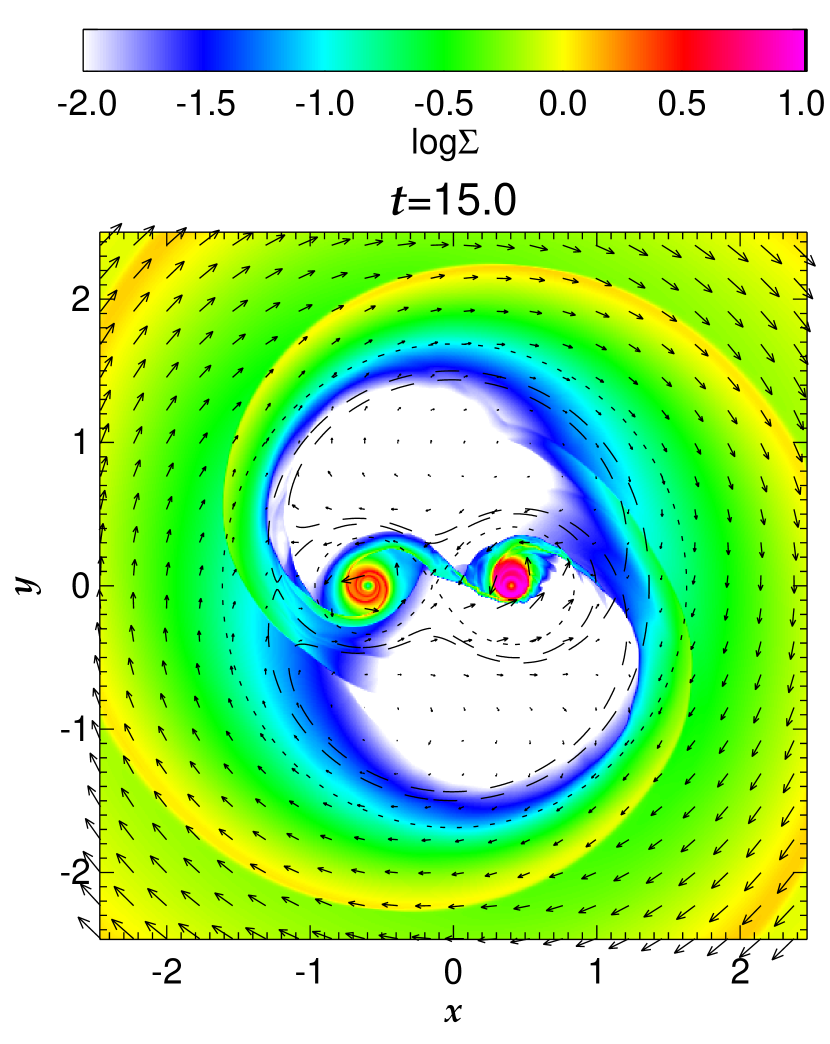
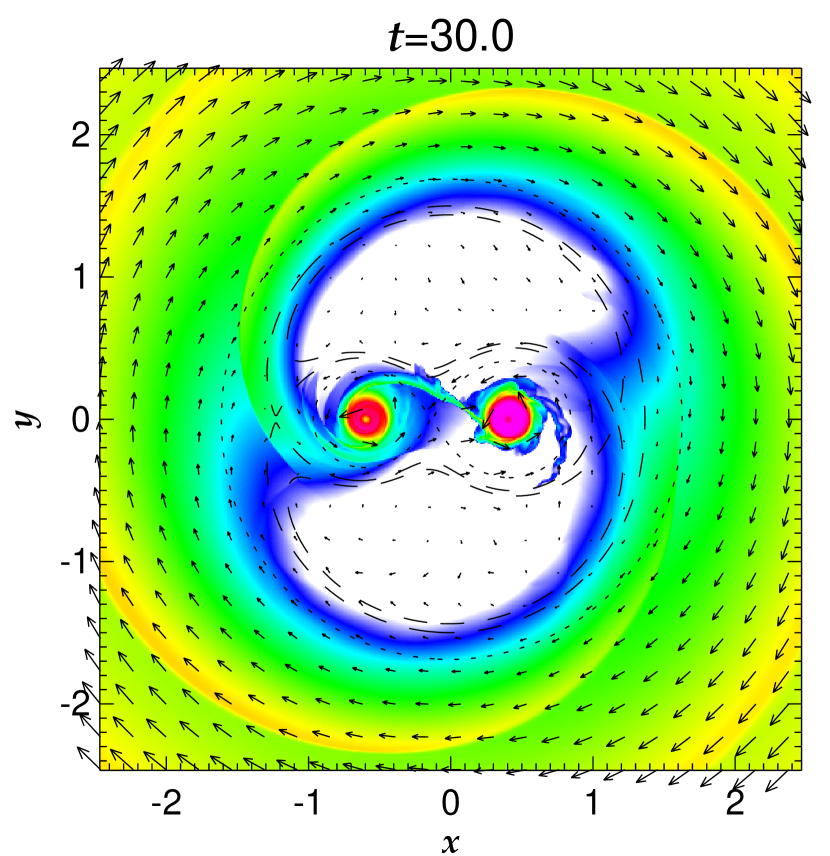
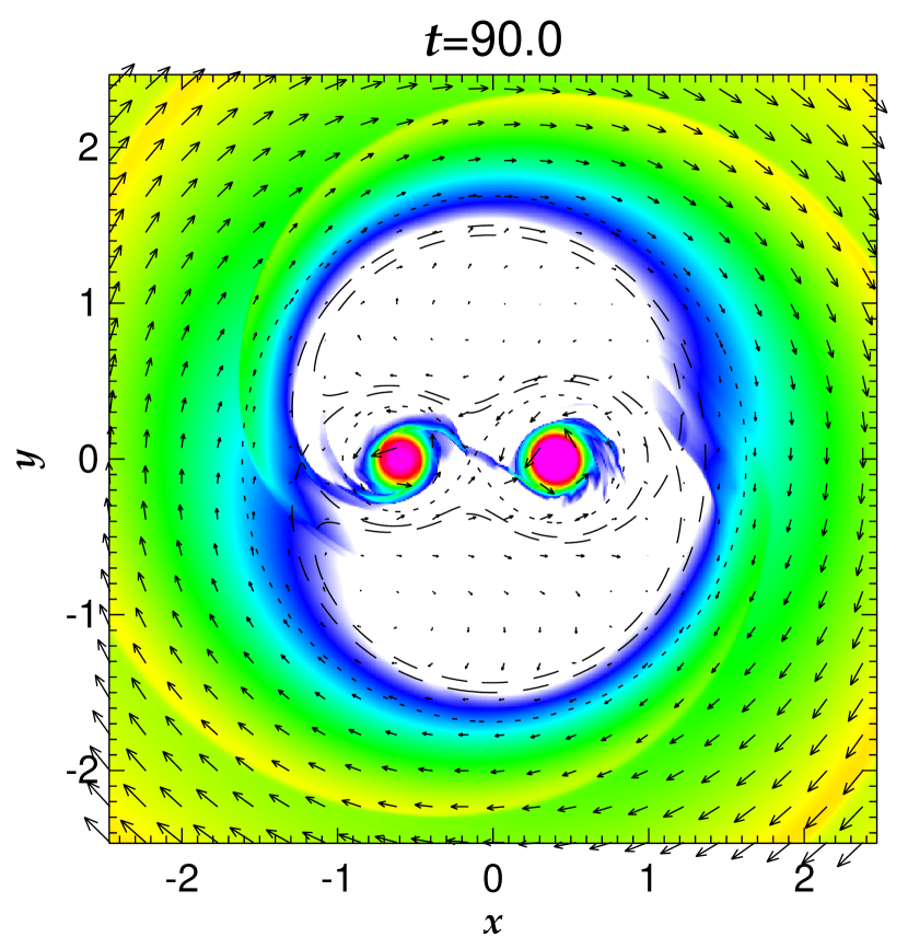
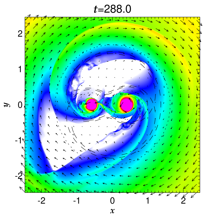
Figure 1: Each panel shows the surface density (color) and velocity distributions at $t$ = 15, 30, 120, and 240 in model 1. The dashed curves are the contours of the Roche potential.

The circumbinary disk has the inner edge at $r\,=\,2.5$ at the initial stage of model 1. Figure 1 shows the surface density distribution at $t$ = 15, 30, 90, and 288 in model 1. The color denotes the surface density in logarithmic scale while the arrows denote the velocity in the frame corotating with binary, $u$. The primary (right) has a more massive circumstellar disk than the secondary (left).

The circumstellar disks accretes gas mainly through L2 point from the circumbinary disk. This is reasonable since the Roche potential is lower at L2 point by $\Delta\Phi\,=\,6.70\times 10^{-2}$. The potential difference is appreciably larger than the square of the sound speed, $c_{s}^{2}\,=\,4.84\times 10^{-2}$. The circumbinary disk has two-armed spiral shock waves (denoted by yellow in Fig. 1).

The gas velocity is small near L2 point. We surmise that it is regulated to be the sound speed, since the Roche potential has a saddle point at L2. Then L2 point should be similar to the throat of Laval nozzle. As well known, the gas velocity coincides with the sound speed at the throat. Similarly the gas velocity should be regulated at the sound speed at L2 point.

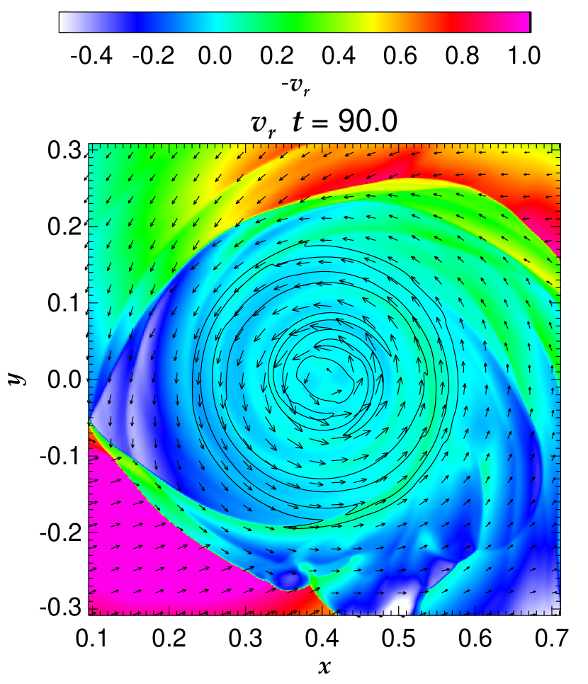
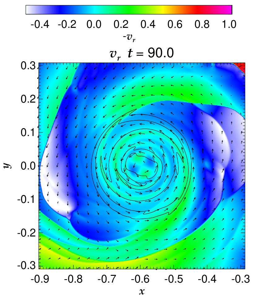
Figure 3: The color denotes the radial velocity toward each star at $t$ = 90.0 in model 1. The left panel denotes the velocity toward the primary, while the right does that toward the secondary.

Figure 2 is a close up view of model 1 at $t$ = 90.0. The left panel is focused on the regions of high surface density while the right is on the regions of low surface density. Spiral shock waves are excited also in the circumstellar disks. The outer part of the primary disk is disturbed appreciably while the secondary is not. The disturbance is likely due to the impact of gas flow from L2. The gas stream is nearly normal to to the primary disk while it is nearly tangential to the secondary disk. See Figure 3 for the radial velocity toward each star. The primary disk receives a larger impact, which produces ‘a hot spot’ on the side closer to L1 point. The radial gas inflow is shown as a function of the azimuthal angle centered on the primary in Figure 4. The ordinate denotes the mass flux, i.e., the product of the surface density and the radial velocity toward the primary at $t$ = 90.0 and $|\mbox{\boldmath$r$}\,-\,\mbox{\boldmath$r$}_{1}|\,=\,0.23$. The azimuthal angle is $\phi$ = 0 and $\pi/2$ in the directions of increasing $x$ and $y$, respectively.

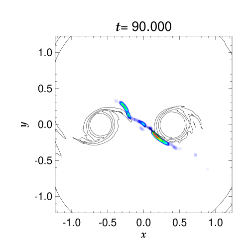
Figure 5: The region of strong shock compression is marked by color on the surface density map at $t$ = 90 in model 1. The colored region is identified by the amplitude of $\mbox{\boldmath$\nabla$}\cdot\mbox{\boldmath$u$}$. It is considerably broadened artificially, since the the shock wave is very sharply resolved and is hard to be recognized in the raw data.

Figure 5 shows the region of large $\mbox{\boldmath$\nabla$}\cdot\mbox{\boldmath$u$}$ at $t$ = 90.0 by color. The colored is the shock front, since the gas is compressed strongly there. It is clearly shown that the primary disk is associated with the strong shock while the secondary disk is not. Furthermore the gas stream changes its density and velocity semi-periodically on a short timescale. The impact on the primary disk varies accordingly.

Note that Figure 2 is different from both the cold and warm SPH models of Delgado-Donate shown in Figure 2 of Clarke (2008). The secondary is surrounded by a shock wave in his cold SPH model while no shock wave is seen in his warm SPH model. The shock location is closely related to the mass accretion rate of each component star. It is crucial whether the gas streaming from L1 point causes a shock around the secondary.

The primary disk mass increases while oscillating appreciably. Figure 6 shows the primary disk mass as a function of time. Each curve denotes the total mass of gas enclosed in a circle around the primary. It also indicates that the surface density falls off sharply around $|\mbox{\boldmath$r$}\,-\,\mbox{\boldmath$r$}_{1}|\,=\,0.2$. Thus we regard the total mass enclosed in the circle of $|\mbox{\boldmath$r$}\,-\,\mbox{\boldmath$r$}_{1}|\,=\,0.2$ as the disk mass in the following.

Figure 7 is the same as Figure 6 but for the secondary disk. The secondary disk mass is smaller than the primary one and increases steadily. The gas flow around the secondary is smooth and the secondary disk accretes gas without significant disturbance.

Semi-periodic change is also seen in the circumbinary disk. Figure 8 shows the time variation in the surface density measured at four points on the axis of $y\,=\,0$. The period of surface density variation is about $P~{}\simeq~{}4.4$ when measured at a given point in the corotation frame. Variation is also seen in the radial velocity. The variation has the temporal and azimuthal dependence of $\cos\,[2(\phi\,-\,\omega t)]$ in the corotation frame, where the angular frequency is approximately $\omega\,\simeq\,0.7\Omega$ in the period $20\,<\,t\,<80$. Around $t\,\simeq\,100$, the surface density variation is not sinusoidal; two waves having similar but different angular frequencies seem to be excited. The amplitude of the wave varies on a longer timescale as shown in Figure 8. It is large in the period $t\,\gtrsim\,130$. This large variation is due to one armed low surface density region shown in the lower right panel of Figure 1.

This quasi-periodic change has not been reported in the literature. It may be missed or smeared out in the previous simulations by some reasons. Paper I and some other simulations assumed continuous dynamical accretion onto the circumbinary disk, which grows the disk and may hinder our perception. Although Günther & Kley (2002) and Günther & Kley (2004) assumed quasi-static initial and boundary conditions, they employed a large empirical viscosity and spatial resolution much lower than ours. The numerical viscosity and relatively low spatial resolution may damp down the quasi-periodic change. We have learned that recent SPH simulations have shown similar variation from Clarke (2009).

Figure 2 shows a thin stripe of high surface density connecting primary and secondary disks as in Paper I. The stripe is formed by the collision of the gas flows rotating around the primary and secondary. In practice, it is the boundary between the domains in one of which the gas flows from secondary to primary and in the other of which it flows vice versa. It is located around L1 point but its location varies with time. When the inflow from L2 has a higher surface density, the stripe is closer to the primary. The location of the stripe is critical to which component of the binary accretes more.

The sum of the disk masses amounts to $M_{\rm 1d}\,+\,M_{\rm 2d}$ = 1.78 at $t$ = 144. This is equal to the mass of the circumbinary ring of $\Delta r$ = 0.11 at $r\,=\,r_{0}$. The total disk mass amounts to $M_{\rm 1d}\,+\,M_{\rm 2d}$ = 4.75 at $t$ = 288.

The time derivative of a disk mass gives us the accretion rate in principle. It is, however, highly variable and hard to read gradual change in the accretion rate. To erase out the short time variability, we obtain the average accretion rate for time intervals of $\Delta t$ = 2.88. Figure 9 shows the average accretion rates for the primary (solid), ${\rm d}M_{\rm 1d}/{\rm d}t$ and secondary (dashed), ${\rm d}M_{\rm 2d}/{\rm d}t$. The accretion rate is very high in the first a few rotation period ($t\,\lesssim\,25)$. The primary has a higher accretion rate than the secondary except around $t\,\simeq\,230$ and 270.

It should be noted that there is correlation between the accretion rates and oscillation in the circumbinary disk. The accretion rates are low when the circumbinary disk is relatively quiet, i.e., around $t~{}\simeq~{}100$. This indicates that the oscillation enhances the accretion from the circumbinary disk through angular momentum exchange.

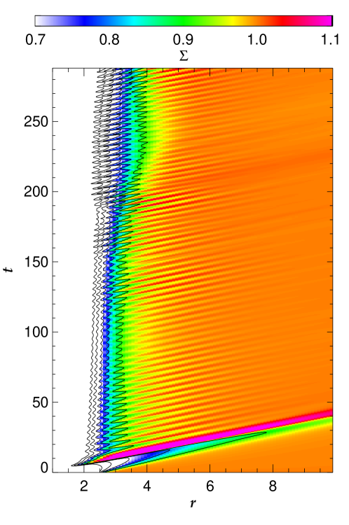
Figure 10: The evolution of the azimuthally averaged surface density of the circumbinary disk in model 1.

Figure 10 shows the azimuthally averaged surface density in the circumbinary disk as a function of $r$ and $t$. It shows repeatedly excited waves propagating outwards of which phase velocity is $dr/dt\,\simeq\,0.25$ and 0.24 at $r$ = 3.2 and 4.2, respectively. The inner edge of the circumbinary disk retreats very slowly. Figure 10 shows that the amplitude of the wave varies on the timescale of several tens rotation period.

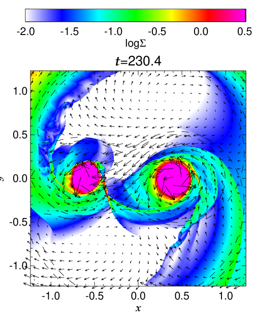
Figure 11: The same as the left panel of Fig. 2 but for the stage of $t$ = 230.4.

At some epochs, the secondary has a higher accretion rate than the primary. Figure 11 shows the flow at $t$ = 230.4 as an example of such a stage. As shown in the figure, the outer part of the circuprimary disk is shed to flow into the secondary lobe. The circumsecondary disk receives the flow and has a hot spot on the L1 point side. Similar mass transfer is also seen around $t\,\simeq\,150$ and 190. The inflow is still mainly through L2 point and the inflow through L3 point is minor. Note that the gas flows from primary to secondary around L1 point in this period. Shortly after this stage, the circumsecondary disk is disturbed very much and captures a gas flow from L2 point. The gas flow inside the Roche lobe is crucial for the branching of the inflow from the circumbinary disk.

3.2 Model 2

We compare model 2 with model 1 to examine the dependence on $r_{0}$, the initial inner radius of the cicumbinary disk. The model parameters of models 2 are the same as those of model 1 except $r_{0}$.

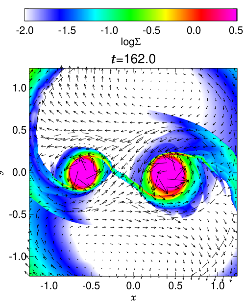
Figure 12: The surface density distribution around the binary at $t$ = 162.0 in model 2.

Figure 12 shows the surface density distributions at $t$ = 162. The circumstellar disk is more massive in model 2 since the circumbinary disk has a smaller inner radius. The primary disk is more massive than the secondary one also in model 2. The primary disk mass increases while oscillating appreciably as shown in Figure 13. The secondary disk mass increases slowly and smoothly as shown in Figure 14. The averaged accretion rate is shown in Figure 15.

3.3 Models 3, 4, and 5

We compare model 4 with model 1 to examine the dependence on the gas temperature. The gas temperature is 29.1% higher in model 3 than in model 1 since the isothermal sound speed is set to be $c_{s}$ = 0.25. It is still lower than the the potential gap between L2 and L3 points. Thus the flow is relatively cold although it is quite higher than that assumed in SPH simulations.

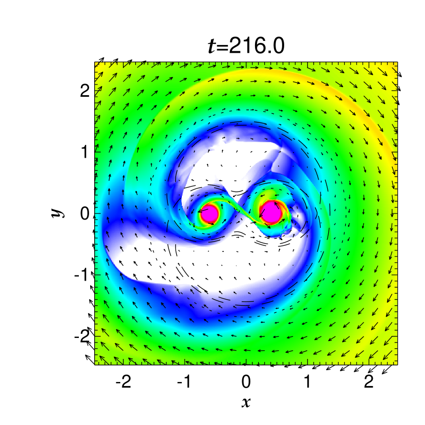
Figure 16: The surface density (color) and velocity (arrows) distributions at $t$ = 108 and 216 in model 3.

Figure 16 shows the distributions of $\Sigma$ and $u$ at $t$ = 108 and 216 in model 3. The spiral arms have a little wider opening angle in the circumbinary disk of model 3 than in that of model 1. The gas inflows mainly from L2 point and the surface density is low around L3 point. Remember that the potential difference is $\Delta\Phi~{}=~{}6.70\times 10^{-2}$ between L2 and L3. It is larger than $c_{s}^{2}$ = $6.25\times 10^{-2}$ also in models 3, 4, and 5.

Figure 17 compares the disk masses of model 3 with those of model 1. Both the primary and secondary disk masses are $\sim$50 % larger in model 4. This is an envidence that the oscillating spiral arms are responsible for the accretion from the circumbinary disk. When $c_{s}$ is higher, the angular momentum exchange should be more effective.

Figure 18 is the same as Figure 17 but for comparison between models 2 and 5 in which only the sound speed, $c_{s}$, is different. The disk masses are $\sim$30 % larger in model 5. When the gas temperature is higher, the accretion rate is higher. The gas temperature affects a little the ratio between the primary and secondary accretion rates.

The vibration of the spiral shock wave is also seen in model 3. Figure 19 is the same as Figure 8 but for model 3. The oscillation frequency is almost the same as that in model 1.

3.4 Model 6

We have constructed model 6 to examine the effect of the softening radius. The initial state is the same as that of model 3 except for $\beta_{1}$ and $\beta_{2}$. The gravity is artificially reduced in the regions of $|\mbox{\boldmath$r$}-\mbox{\boldmath$r$}_{1}|<0.14$ and $|\mbox{\boldmath$r$}-\mbox{\boldmath$r$}_{2}|<0.14$ in model 6.

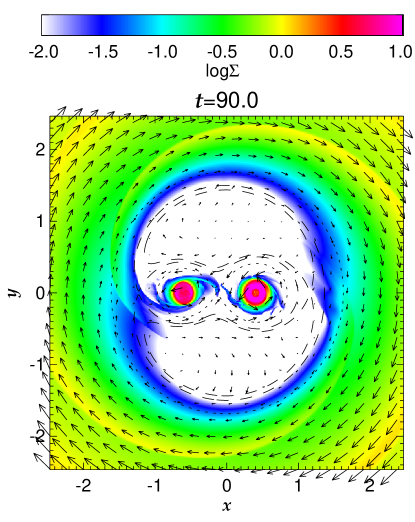
Figure 20: The surface density distribution at $t$ = 90.0 in model 6. The notation is the same as that of Fig. 1.

Figure 20 shows the surface density distribution at $t$ = 90.0 in model 6. Also in model 6, the the primary disk is more massive than the secondary one. Since the gravity is artificially reduced in a larger area, the primary and secondary disks are rings with larger holes in the early stages. It takes a longer time for the gas rings to spread into the center.

Figures 21 and 22 are the same as Figures 6 and  7 but for the primary and secondary disks in model 6, respectively. The mass of the secondary disk is smaller than in model 3. Note, however, that the softening radius is still as small as $\beta_{2}$ = 0.14. The secondary disk extends outside the softening radius and can capture gas if it is accreted. The primary disk sheds its outer part at some epochs (e.g. $t\simeq 150$ and 190) and the secondary receives it. This feature is also seen in model 6.

The softening radius affects the inner structure of the circumstellar disks. However, it does not affect the gas stream from L₂ point directly; the gas flows far from the region of artificial reduction in the gravity. We conclude that the softening radius does not give a serious effect on the result that the primary accretes more than the secondary.

3.5 Model 7

We have constructed model 7 to examine the effect of initial surface density distribution. Model 7 is the same model 2 except for $h$ which denotes the surface density gradient at the initial disk edge. The surface density increases gradually in model 7 since $h~{}=~{}0.6$. Hence the initial pressure force is much weaker than in model 2, since $h~{}=~{}0.144$ in model 2.

Figures 23 and 24 show the disk mass as a function of time in model 7 for primary and secondy, respectively. The initial rise in the primary disk mass is steeper in model 7. This is because the initial disk is extended more in model 7. Inner part of the circumbirnary disk is truncated even when the pressure gradient is weak. The primary disk mass of model 7 is almost the same as that of model 2. The disk mass does not depend seriously on $h$.

4 DISCUSSIONS

In this section, we discuss the softening radius, the hot spot, the accretion impact on the circumstellar disk, and the oscillation of spiral waves excited in the circumbinary disk.

In this work the softening radii, $\beta_{1}$ and $\beta_{2}$, are three times smaller than those in our previous work (Paper I). They are also much smaller than the circumstellar disk radii. Our numerical simulations clearly resolved internal structures of the circumstellar disks such as spiral waves within them. The simulations still depend a little on the softening radius. The gas accretion is slow inside the softening radii and the circumstellar disks have inner holes in the early period. The circumstellar disks affect accretion rates through dynamical interaction with the gas stream from L2 point.

Further reduction in the softening radius requires extremely high spatial resolution and accordingly unfeasible computation cost. See Appendix on the spatial resolution required.

As shown in the previous section, the primary disk has a hot spot during the primary accretion rate dominates over the secondary one. The hot spot is due to the impact of the gas stream and the gas looses its kinetic energy through shock dissipation. The kinetic energy dissipation plays an important role for a gas element to be accreted onto a circumstellar disk.

It is well known that the Jacobi integral,

$$J\;=\;\frac{|\mbox{\boldmath$u$}|^{2}}{2}\;+\;\Phi\,,$$ (9)

is a constant of motion for a particle moving around a circular binary. After some algebraic manipulation, we obtain

$$\frac{DJ^{\prime}}{Dt}\;=\;-\,c_{s}^{2}\,\frac{\partial\ln\Sigma}{\partial t}\,$$ (10)

for an isothermal gas flow without shock, where

$$J^{\prime}\;=\;J\;+\;c_{s}^{2}\,\ln\Sigma.$$ (11)

The difference between $J$ and $J^{\prime}$ is small when the gas temperature is low. The right hand side of Equation (10) is also small. Thus the Jacobi integral can be regarded as a constant for a Lagrangian gas element if the gas is cold. When a particle orbits around the primary at the Keplerian velocity, the Jacobi integral is evaluated to be

$$J_{1}\;=\;-\,M_{2}\,-\,\frac{M_{2}^{2}}{2}\,+\,\frac{1}{2}\left(\sqrt{\displaystyle\frac{M_{1}}{|\mbox{\boldmath$r$}\,-\,\mbox{\boldmath$r$}_{1}|}}\,-\,|\mbox{\boldmath$r$}\,-\,\mbox{\boldmath$r$}_{1}|\right)^{2}\,,$$ (12)

where the tidal force due to the secondary is neglected for simplicity. Similarly, it is evaluated to be

$$J_{2}\;=\;-\,M_{1}\,-\,\frac{M_{1}^{2}}{2}\,+\,\frac{1}{2}\left(\sqrt{\displaystyle\frac{M_{2}}{|\mbox{\boldmath$r$}\,-\,\mbox{\boldmath$r$}_{2}|}}\,-\,|\mbox{\boldmath$r$}\,-\,\mbox{\boldmath$r$}_{2}|\right)^{2}\,,$$ (13)

for a particle orbiting around the secondary. The values of $J_{1}$ and $J_{2}$ are shown as a function of the orbital radius in Figure 25. The dashed lines denote the potential energy at the Lagrangian points L₁, L₂, and L₃.

The inflowing gas has a small velocity in the corotation frame when it passes L₂ point. Thus the Jacobi integral is nearly equal to the potential energy at L₂ point. Provided that the gas accretes onto either the primary or the secondary without changing the Jacobi integral. Then the orbital radius should be as much as $|\mbox{\boldmath$r$}\,-\,\mbox{\boldmath$r$}_{1}|$ = 0.34 or $|\mbox{\boldmath$r$}\,-\,\mbox{\boldmath$r$}_{2}|$ = 0.30. The orbital radius can be smaller only when the Jacobi integral is reduced substantially through strong shock dissipation.

When the orbital radius is $|\mbox{\boldmath$r$}\,-\,\mbox{\boldmath$r$}_{1}|$ = 0.26, the Jacobi integral, $J_{1}$, is equal to that at rest at L₁ point. This implies that a gas element is marginally bound to the primary when the orbital radius is 0.26. The gas element may flows into the secondary lobe if perturbed a little. Our simulations indeed show such mass transfer from the primary disk to the secondary one around $t~{}\simeq~{}190$ in model 1. The outer part of primary disk is shed into the secondary. The radius of the marginally bound orbit is $|\mbox{\boldmath$r$}\,-\,\mbox{\boldmath$r$}_{2}|$ = 0.21 for the secondary disk. The secondary disk is confined mostly inside the marginal orbit in our simulations.

The above discussion gives a guideline for choosing the softening radius. A gas element orbiting at the softening radius should have an appreciably smaller Jacobi integral than resting at L1 point. If the gas element has an eccentric orbit around a star, the pericenter should be located outside the softening radius. Since the softening radius was 20 % of the binary separation in Paper I, it is close to the radius of the marginally bound orbit for the secondary and should be set smaller.

The kinetic energy dissipation may brighten the hot spot at some wavelengths. Although the hot spot is assumed to be isothermal in our simulations for simplicity, it should be hotter than the rest part of the circumstellar disk. It should be analogous to the hot spot in the cataclysmic variables and X-ray binaries (see, e.g., Marsh, 2001). In these systems, a compact star (either of white dwarf, neutron star and black hole) accretes gas from its companion through L₁ point. The gas inflow forms a hot spot on the circumstellar disk around the compact star. It is often identified by occultation. Similarly, the hot spot may be observed in binaries of young stellar objects. It may be identified by the Doppler effect if it is luminous at some emission lines.

It should be noted that the impact depends on the circumprimary disk. When the circumprimary disk has a higher surface density and pressure, the inflowing gas stream is relatively weaker and hence produces the impact point at an outer radius. The evolution of circumstellar disks is controlled by angular momentum transfer and hence will be affected by assumed viscosity and gravity softening.

Next we discuss the oscillation of spiral waves excited in the circumbinary disk. The oscillation is closely related to gas accretion from the circumbinary disk as shown in the previous section. This is also confirmed by Equation (10). If the density distribution is stationary in the corotation frame, the modified Jacobi constant, $J^{\prime}$, is constant except when it gets across a shock front. The shock dissipates the kinetic energy and decreases the Jacobi constant. If the Jacobi constant decreases, the orbital radius increases. This is because the Jacobi constant is evaluated to be

$$J\;=\;-\,\frac{1}{2r}\,-\,\sqrt{r}\,,$$ (14)

when the gas element rotates around the binary with the orbital radius, $r$, in the circumbinary disk. Equation (14) is derived under the assumption that the orbit is almost circular and the velocity is Keplerian. The Jacobi constant is larger for a larger $r$ when $r\,>\,1$. In other words, the gas element gains angular momentum from the spiral wave corotating with the binary, since the angular velocity of the binary is higher than that of a gas element in the circumbinary disk. This means that a stationary shock wave drives the circumbinary disk outward. The accretion is due to vibration of the shock wave. Some gas elements move inward by loosing the angular momentum and Jacobi constants through exchange with some other gas elements, when the spiral shock wave is not stationary.

The oscillation has a typical period of $\sim 4.5$ when measured in the corotation frame. Accordingly the wave has an apparent phase velocity of $\sim 0.7$ in the corotation frame since the azimuthal wavenumber is $m=2$. Then the phase velocity is $\sim 0.3$ in the rest frame and coincides with the angular velocity of gas orbiting around the binary at $r\,\simeq\,2.2$. This implies that the wave is excited by resonance at the inner edge of the circumbinary disk.

The amplitude of the oscillation varies on the timescale of several tens rotation period. The variation is coherent in the radial direction. When the amplitude is small, the whole cicumbinary disk is nearly stationary. When the amplitude is large, both the radial and azimuthal components of velocity oscillate at the same frequency. The variation may induce variability in the accretion onto the binary.

Appendix A REFERENCE VELOCITY METHOD

We describe the reference velocity methods for integrating hydrodynamical equations.

First we divide the computation domain into four areas: one around the primary, another around the secondary, another surrounding the binary, and the rest. The reference velocity is defined differently in each area.

The reference velocity is defined to be the Keplerian rotation around the center of mass,

$$\mbox{\boldmath$w$}\;=\;\omega(|\mbox{\boldmath$r$}|)\,\mbox{\boldmath$e$}_{z}\times\mbox{\boldmath$r$}$$ (A1)

$$\omega(r)=-1+r^{-3/2},$$ (A2)

outside the circle of $|\mbox{\boldmath$r$}|\geq 1$.

The reference velocity is taken to be circular rotation around the primary,

$$\mbox{\boldmath$w$}\;=\;\omega(|\mbox{\boldmath$r$}\,-\,\mbox{\boldmath$r$}_{1}|)\,\mbox{\boldmath$e$}_{z}\times\left(\mbox{\boldmath$r$}\,-\,\mbox{\boldmath$r$}_{1}\right)\,$$ (A3)

in the vicinity of $|\mbox{\boldmath$r$}\,-\,\mbox{\boldmath$r$}_{1}|\,\leq\,\gamma_{1}$. The angular velocity is set to be

$$\omega\left(|\mbox{\boldmath$r$}\,-\,\mbox{\boldmath$r$}_{1}|\right)\;=\;\left\{\begin{array}[]{ll}-\,\Omega\,+\,\displaystyle\left(\frac{M_{1}}{\beta_{1}^{3}}\right)^{1/2}\,\left[\frac{7}{4}\,-\,\frac{3}{4}\,\left(\frac{|\mbox{\boldmath$r$}\,-\,\mbox{\boldmath$r$}_{1}|}{\beta_{2}}\right)^{2}\right]&\left(|\mbox{\boldmath$r$}\,-\,\mbox{\boldmath$r$}_{1}|\,<\,\beta_{1}\right)\\ -\,\Omega\,+\,\displaystyle\left(\frac{M_{1}}{|\mbox{\boldmath$r$}\,-\,\mbox{\boldmath$r$}_{1}|^{3}}\right)^{1/2}&\left(\beta_{1}\,\leq\,|\mbox{\boldmath$r$}\,-\,\mbox{\boldmath$r$}_{1}|\,\leq\,\alpha_{1}\right)\\ -\,\Omega\,+\,\displaystyle\left(\frac{M_{1}}{\alpha_{1}^{3}}\right)^{1/2}\,\left(\frac{5}{2}\,-\,\frac{3}{2}\frac{|\mbox{\boldmath$r$}\,-\,\mbox{\boldmath$r$}_{1}|}{\alpha_{1}}\right)&\left(\alpha_{1}\,<\,|\mbox{\boldmath$r$}\,-\,\mbox{\boldmath$r$}_{1}|\,<\,\gamma_{1}\right)\end{array}\right..$$ (A4)

The angular velocity coincides with the Keplerian velocity around the primary in the region of $\beta_{1}\,\leq\,r_{1}\,\leq\,\alpha_{1}$. It is slower than the Keplerian velocity in the region of $\alpha_{1}\,\leq\,r_{1}\,\leq\,\gamma_{1}$. The radius, $\gamma_{1}$, is set to be

$$\gamma_{1}\;=\;\frac{2\alpha_{1}}{3}\,\left[\frac{5}{2}\,\left(\frac{M_{1}}{\alpha_{1}^{3}}\right)\,-\,\Omega\right]\,,$$ (A5)

so that the angular velocity vanishes at $|\mbox{\boldmath$r$}\,-\,\mbox{\boldmath$r$}_{1}|\,=\,\gamma_{1}$.

The gravity of the primary is softened so that it balances with the centrifugal force due to the reference velocity. Thus the gravity due to the primary is reduced to

$$\mbox{\boldmath$g$}\left(|\mbox{\boldmath$r$}\,-\,\mbox{\boldmath$r$}_{1}|\right)\;=\;-\,\frac{M_{1}}{\beta_{1}{}^{3}}\,\left(\mbox{\boldmath$r$}\,-\,\mbox{\boldmath$r$}_{1}\right)\,\left[\frac{7}{4}\,-\,\frac{|\mbox{\boldmath$r$}\,-\,\mbox{\boldmath$r$}_{1}|}{\beta_{2}{}^{2}}\right]\,.$$ (A6)

Similarly the reference velocity is taken to be circular rotation around the secondary in the vicinity of the secondary. It is expressed as

$$\mbox{\boldmath$w$}\;=\;\omega(|\mbox{\boldmath$r$}\,-\,\mbox{\boldmath$r$}_{2}|)\,\mbox{\boldmath$e$}_{z}\times\left(\mbox{\boldmath$r$}\,-\,\mbox{\boldmath$r$}_{2}\right)$$ (A7)

$$\omega(|\mbox{\boldmath$r$}\,-\,\mbox{\boldmath$r$}_{2}|)\;=\;\left\{\begin{array}[]{ll}-\,\Omega\,+\,\displaystyle\left(\frac{M_{2}}{\beta_{2}^{3}}\right)^{1/2}\,\left[\frac{7}{4}\,-\,\frac{3}{4}\,\left(\frac{|\mbox{\boldmath$r$}\,-\,\mbox{\boldmath$r$}_{2}|}{\beta_{2}}\right)^{2}\right]&(|\mbox{\boldmath$r$}\,-\,\mbox{\boldmath$r$}_{2}|\,<\,\beta_{2})\\ -\,\Omega\,+\,\displaystyle\left(\frac{M_{2}}{|\mbox{\boldmath$r$}\,-\,\mbox{\boldmath$r$}_{2}|^{3}}\right)^{1/2}&(\beta_{2}\,\leq\,|\mbox{\boldmath$r$}\,-\,\mbox{\boldmath$r$}_{2}|\,\leq\,\alpha_{2})\\ -\,\Omega\,+\,\displaystyle\left(\frac{M_{2}}{\alpha_{2}^{3}}\right)^{1/2}\,\left(\frac{5}{2}\,-\,\frac{3}{2}\frac{|\mbox{\boldmath$r$}\,-\,\mbox{\boldmath$r$}_{2}|}{\alpha_{2}}\right)&(\alpha_{2}\,<\,|\mbox{\boldmath$r$}\,-\,\mbox{\boldmath$r$}_{2}|\,<\,\gamma_{2})\end{array}\right.\,$$ (A8)

where

$$\gamma_{2}\;=\;\frac{2\alpha_{2}}{3}\,\left[\frac{5}{2}\,\left(\frac{M_{2}}{\alpha_{2}^{3}}\right)\,-\,\Omega\right]\,,$$ (A9)

The values of $\alpha_{i}$, $\beta_{i}$, and $\gamma_{i}$ are tabulated in Table 2. Note $\gamma_{1}\,+\,\gamma_{2}\,<\,1$ and accordingly that the region of $|\mbox{\boldmath$r$}\,-\,\mbox{\boldmath$r$}_{1}|\,<\,\gamma_{1}$ does not overlap with that of $|\mbox{\boldmath$r$}\,-\,\mbox{\boldmath$r$}_{2}|\,<\,\gamma_{2}$.

The reference velocity vanishes in the rest area, i.e., inside the circumbinary disk but outside the primary and secondary disks. Remember that the reference velocity is continuous even on the boundary between the different areas. Thus the derivative of the reference velocity is regular and continuous except discontinuity on the boundary between the areas.

The discontinuity of the reference velocity derivative has no serious effect on the evaluation of the source term. The reference velocity is analogous to the vector potential in the electromagnetism. Thus its derivative is analogous to the magnetic field. The magnetic field can be discontinuous so the derivative of the the reference velocity can be. Remember that the reference velocity is divergence free, $\mbox{\boldmath$\nabla$}\cdot\mbox{\boldmath$w$}\,=\,0$. This is analogous to the Coulomb gauge in the electromagnetism.

The numerical flux is evaluated at the cell surface as in the ordinary finite volume method. The reference velocity is evaluated analytically at the cell surface while the other variables are evaluated from the cell center values by using interpolation with the minmod limiter. Then the reference velocity is numerical viscosity free and the numerical solution has a larger Reynolds number.

Introduction of the reference velocity improves evaluation of the centrifugal force greatly. The centrifugal force, $v\cdot\nabla v$, contains a spatial derivative of the velocity. The spatial derivative is evaluated from the spatial difference in an ordinary finite difference method and truncation error is inevitable in its numerical evaluation. The truncation error should be small so that minor forces such as pressure force are appreciated properly. Note that the numerical derivative is only the first order accurate near shock fronts in a TVD scheme (Toro, 2009, see, e.g.,). When and only when the spatial resolution, $\Delta x$, is much smaller than the the scaleheight,

$$\Delta x\;\ll\;\frac{c_{s}^{2}\,r^{2}}{GM}\,$$ (A10)

the truncation error is ensured to be much smaller than the pressure force. This condition is equivalent to

$$\Delta x\;\ll\;\left(\frac{c_{s}}{v_{K}}\right)^{2}\,r\;,$$ (A11)

where $v_{K}$ denotes the Keplerian velocity.

The reference velocity relaxes the above mentioned requirement on the truncation error. Alternatively, the resolution should be so small that the difference in reference velocity is smaller than the sound speed between any adjacent cells. Otherwise a gas element would be accelerated (or decelerated) too much by advection from a cell to another. This requirement is less tight, since it can be expressed as

$$\Delta x\;\ll\;\left(\frac{c_{s}}{v_{K}}\right)\,r\;.$$ (A12)

Equation (A11) is much more tight than this, when the Mach number ($v_{K}/c_{s}$) is large. The Mach number is as high as

$$\frac{v_{K}}{c_{s}}\;=\;13.3\left(\frac{M_{1}}{0.596}\right)^{1/2}\,\left(\frac{|\mbox{\boldmath$r$}\,-\,\mbox{\boldmath$r$}_{1}|}{0.07}\right)^{-1/2}\,\left(\frac{c_{s}}{0.22}\right)^{-1}\,$$ (A13)

for the Keplerian rotation around the primary. Thus the reference velocity. Further reduction in the softening radius requires extremely high spatial resolution even when the reference velocity is introduced.

Our numerical scheme is similar to FARGO (Fast Advection in Rotating Gaseous Objects) developed by Masset (2000) for solving hydrodynamics a gaseous disk rotating around a star on fixed polar grids. FARGO decomposes the rotation velocity into two components, the azimuthally averaged rotation and deviation from it. The advection due to the former is treated separately in FARGO. The separation relaxes the ordinary Courant condition and speeds up the computation. At the same time, numerical diffusivity is much smaller in FARGO thanks to the two step advection. The centrifugal force is dominated by that due to the averaged rotation, $J^{2}/r^{3}$, where $J$ denotes the specific angular momentum. Thus the truncation error is reduced also in FARGO.

The reference velocity is, however, different from FARGO. Application of FARGO is limited to the case that the grid is set almost parallel to the gas flow. The reference velocity method can be applied to any numerical grids. FARGO can take a long time step while the reference velocity method can not.

Our numerical scheme is also similar to that of LeVeque (1998). He proposed a scheme to take account of gradient of a physical variable within a numerical cell for elliminating source terms apparently. In case of hydrodynamics, the gravity can be taken into account if the pressure has different values at the cell surfaces opposing each other. Our reference velocity has different values at the cell surfaces to incorporate the gravity. His scheme is effective for a flow in a quasi-static balance while ours is effective for a flow supported mainly by the centrifugal force.

Figure 4: The solid curve denotes the radial mass flux, $\Sigma v_{r1}$, onto the primary disk as a function of the azimuthal angle, $\phi_{1}\,=\,\tan^{-1}[y/(x\,-\,x_{1})]$, where $v_{r1}$ denotes the radial velocity with respect to the primary. The dashed curve is the same as the solid one but for the secondary.

Figure 6: Each curve denotes the total mass of gas inside a circle around the primary as a function of time. The numbers denote the radii of the circles.

Figure 7: The same as Fig. 6 but for the secondary.

Figure 8: The time variation of the surface density on the axis of $y$ = 0 in model 1.

Figure 9: The accretion rates of the primary and secondary derived from the best fit polynomials to their disk masses.

Figure 13: The same as Fig. 6 but for model 2.

Figure 14: The same ad Fig. 7 but for the secondary disk in model 2.

Figure 15: The same ad Fig. 9 but model 2.

Figure 17: The comparison of disk masses between model 1 (thin) and 3 (thick). The solid curves denote the primary disk mass while the dashed do the secondary one.

Figure 18: The same as Fig. 17 but for comparison model 2 (thin) and 5 (thick).

Figure 19: The same as Fig. 8 but for model 4.

Figure 21: The same ad Fig. 6 but for the primary in model 6.

Figure 22: The same ad Fig. 6 but for the secondary in model 6.

Figure 23: The same ad Fig. 13 but for that in model 7.

Figure 24: The same ad Fig. 14 but for model 7.

Figure 25: The Jacobi integral is shown for circular orbits around the primary (solid) and secondary (dashed). The abscissa is the orbital radius. The value of Jacobi integral is also shwon for particles at rest on the Lagrangian points, L₁, L₂, and L₃ for reference.

No.	$c_{s}$	$r_{0}$	$H$	$\beta_{1}~{}(=~{}\beta_{2})$
1	0.22	2.5	0.144	0.07
2	0.22	2.1	0.144	0.07
3	0.25	2.5	0.144	0.07
4	0.25	2.3	0.144	0.07
5	0.25	2.1	0.144	0.07
6	0.22	2.5	0.144	0.14
7	0.22	2.1	0.600	0.07

Table 1: Summary of models.

$i$	1	2
$M_{i}$	0.5957	0.4043
$\alpha_{i}$	0.4000	0.2700
$\gamma_{i}$	0.5793	0.41028

Table 2: Model parameters for the reference velocity.

References

- Artymowicz & Lubow (1996) Artymowicz, P., Lubow, S. H. 1996, ApJ, 467, L77
- Bate & Bonnnell (1997) Bate, M. R., & Bonnell, I. A. 1997, MNRAS, 285, 33
- Clarke (2008) Clarke, C. J. 2008, Pathways Through an Eclectic Universe (Eds. J. H. Knapen, T.J. Mahoney, A. Vaszdekis; ASP Conf. Ser. Vol.390) 76C
- Clarke (2009) Clarke, C. J. 2009, private communication
- Delgado-Donate et al. (2004) Delgado-Donate, E. J., Clarke, C. J., Bate, M. R., & Hodgkin, S. T. 2004, MNRAS, 351, 667
- Delgad-Doanate (2004) Delgado-Donate, E. J., & Clarke, C. J. 2005, Astron. Nach., 10, 94
- Ducchêne et al. (2007) Duchêne, G., Delgado-Donate, E., Haisch, K. E., Jr., Loinard, L., & Rodríguez, L. F. 2007, in Protostars and Planets V, ed. B. Reipurth, D. Jewitt, & K. Keil (Tucson: Univ. Arizona Press), 379
- Duquennoy & Mayor (1991) Duquennoy, A. & Mayor, M. 1991, å, 248, 445
- Günther & Kley (2002) Günther, R., & Kley, W. 2002, å, 387, 550
- Günther & Kley (2004) Günther, R., & Kley, W. 2004, å, 423, 559
- Hioki et al. (2007) Hioki, T., Itoh, Y., Oasa, Y., Fukagawa, M., Kudo, T., Mayama, S. Funayama, H., Hayashi, M., Hayashi, S., Pyo, T.-S., Ishii, M., Nishikawa, T., & Tamura, M. 2008, AJ, 134, 880
- Ireland & Kraus (2008) Ireland, M. J., & Kraus, A. L. 2008, ApJ, 678, L59
- LeVeque (1998) LeVeque, R. J 1998, J. Comp. Phys., 146, 346
- Marsh (2001) Marsh, T. R. 2001, Binary Stars: Selected Topics in Observations and Physical Processes, ed. F. C. Lázaro and M. J. Arévalo (Springer, Berlin) Chap. 4.
- Masset (2000) Masset, F. 2000, A&A, 141, 165
- Ochi et al. (2005) Ochi, Y., Sugimoto, K., & Hanawa, T. 2005, ApJ, 623, 922 (Paper I)
- Reid & Gizis (1997) Reid, N., & Gizis, J. E. 1997, AJ, 113, 2246
- Toro (2009) Toro, E., Riemann Solvers and Numerical Methods for Fluid Dynamics, 3rd Ed. (Springer, Dordrecht) p. 448