Amplification arguments for large sieve inequalities

Abstract.

We give a new proof of the arithmetic large sieve inequality based on an amplification argument, and use a similar method to prove a new sieve inequality for classical holomorphic cusp forms. A sample application of the latter is also given.

1. The classical large sieve

The classical arithmetic large sieve inequality states that, for any real numbers $N$, $Q\geqslant 1$, any choice of subsets $\Omega_{p}\subset\mathbf{Z}/p\mathbf{Z}$ for primes $p\leqslant Q$, we have

(1) $$|\{n\leqslant N\,\mid\,n\,(\mathrm{mod}\,{p})\notin\Omega_{p}\text{ for }p\leqslant Q\}|\leqslant\frac{\Delta}{H}$$

where

$$H=\mathop{\sum\Bigl{.}^{\flat}}\limits_{q\leqslant Q}{\prod_{p\mid q}{\frac{|\Omega_{p}|}{p-|\Omega_{p}|}}},$$

and $\Delta$ is any constant for which the “harmonic” large sieve inequality holds: for any complex numbers $(a_{n})$, we have

(2) $$\sum_{q\leqslant Q}{\mathop{\sum\Bigl{.}^{*}}\limits_{a\,(\mathrm{mod}\,{q})}{\Bigl{|}\sum_{n\leqslant N}{a_{n}e\Bigl{(}\frac{an}{q}\Bigr{)}}\Bigr{|}^{2}}}\leqslant\Delta\sum_{n\leqslant N}{|a_{n}|^{2}},$$

the notation $\mathop{\sum\Bigl{.}^{\flat}}\limits$ and $\mathop{\sum\Bigl{.}^{*}}\limits$ denoting, respectively, a sum over squarefree integers, and one over integers coprime with the (implicit) modulus, which is $q$ here.

By work of Montgomery-Vaughan and Selberg, it is known that one can take

$$\Delta=Q^{2}-1+N$$

(see, e.g., [7, Th. 7.7]).

There are a number of derivations of (1) from (2); for one of the earliest, see [10, Ch. 3]. The most commonly used is probably the argument of Gallagher involving a “submultiplicative” property of some arithmetic function (see, e.g., [8, §2.2] for a very general version).

We will show in this note how to prove (1) quite straightforwardly from the dual version of the harmonic large sieve inequality: $\Delta$ is also any constant for which

(3) $$\sum_{n\leqslant N}{\Bigl{|}\sum_{q\leqslant Q}{\mathop{\sum\Bigl{.}^{*}}\limits_{a\,(\mathrm{mod}\,{q})}{\beta(q,a)e\Bigl{(}\frac{an}{q}\Bigr{)}}}\Bigr{|}^{2}}\leqslant\Delta\sum_{q\leqslant Q}{\mathop{\sum\Bigl{.}^{*}}\limits_{a\,(\mathrm{mod}\,{q})}{|\beta(q,a)|^{2}}},$$

holds for arbitrary complex numbers $(\beta(q,a))$. This is of some interest because, quite often, the inequality (2) is proved by duality from (3), and because, in recent generalized versions of the large sieve (see [8]), it often seems that the analogue of (3) is the most natural inequality to prove – or least, the most easily accessible. So, in some sense, one could dispense entirely with (2) for many applications! In particular, note that both known proofs of the optimal version with $\Delta=N-1+Q^{2}$ proceed by duality.

Note that some ingredients of many previous proofs occur in this new argument. Also, there are other proofs of (1) working directly from the inequality (3) which can be found in the older literature on the large sieve, usually with explicit connections with the Selberg sieve (see the references to papers of Huxley, Kobayashi, Matthews and Motohashi in [11, p. 561]), although none of those that the author has seen seems to give an argument which is exactly identical or as well motivated. Also, traces of this argument appear earlier in some situations involving modular forms, e.g., in [4]. In Section 2, we will use the same method to obtain a new type of sieve inequality for modular forms; in that case, it doesn’t seem possible to adapt easily the classical proofs.

Indeed, maybe the most interesting aspect of our proof is that it is very easy to motivate. It flows very nicely from an attempt to improve the earlier inequality

(4) $$|\{n\leqslant N\,\mid\,n\,(\mathrm{mod}\,{p})\notin\Omega_{p}\text{ for }p\leqslant Q\}|\leqslant\frac{\Delta}{K},\quad\quad K=\sum_{p\leqslant Q}{\frac{|\Omega_{p}|}{p}},$$

of Rényi, which is most easily proved using (3) instead of (1), as in [8, §2.4].

We will explain this quite leisurely; one could be much more concise and direct (as in Section 2).

Let

$$S=\{n\leqslant N\,\mid\,n\,(\mathrm{mod}\,{p})\notin\Omega_{p}\text{ for }p\leqslant Q\},$$

be the sifted set; we wish to estimate from above the cardinality of this finite set. From (3), the idea is to find an “amplifier” of those integers remaining in the sifted set, i.e., an expression of the form

$$A(n)=\sum_{q\leqslant Q}{\mathop{\sum\Bigl{.}^{*}}\limits_{a\,(\mathrm{mod}\,{q})}{\beta(q,a)e\Bigl{(}\frac{an}{q}\Bigr{)}}}$$

which is large (in some sense) when $n\in S$. Then an estimate for $|S|$ follows from the usual Chebychev-type manoeuvre.

To construct the amplifier $A(n)$, we look first at a single prime $p\leqslant Q$. If $n\in S$, we have $n\,(\mathrm{mod}\,{p})\notin\Omega_{p}$. If we expand the characteristic function of $\Omega_{p}$ in terms of additive characters, we have then

$$0=\mathbf{1}_{\Omega_{p}}(n)=\sum_{a\,(\mathrm{mod}\,{p})}{\alpha(p,a)e\Bigl{(}\frac{an}{p}\Bigr{)}},\quad\quad\quad\alpha(p,a)=\frac{1}{p}\sum_{x\in\mathbf{Z}/p\mathbf{Z}}{\mathbf{1}_{\Omega_{p}}(x)e\Bigl{(}\frac{ax}{p}\Bigr{)}},$$

and the point is that the contribution of the constant function ($0$-th harmonic) is, indeed, relatively “large”, because it is

$$\alpha(p,0)=\frac{|\Omega_{p}|}{p},$$

and exactly reflects the probability of a random element being in $\Omega_{p}$. Thus for $n\,(\mathrm{mod}\,{p})\notin\Omega_{p}$, we have

(5) $$\mathop{\sum\Bigl{.}^{*}}\limits_{a\,(\mathrm{mod}\,{p})}{\beta(p,a)e\Bigl{(}\frac{an}{p}\Bigr{)}}=c_{p}$$

with

$$c_{p}=\frac{|\Omega_{p}|}{p},\quad\quad\beta(p,a)=-\alpha(p,a).$$

If we only use the contribution of the primes in (3), and the amplifier

$$A(n)=\sum_{p\leqslant Q}{\sum_{a\,(\mathrm{mod}\,{p})}{\beta(p,a)e\Bigl{(}\frac{an}{p}\Bigr{)}}},$$

then by (3), we get

$$\sum_{n\in S}{|A(n)|^{2}}\leqslant\sum_{n\leqslant N}{|A(n)|^{2}}\leqslant\Delta\sum_{p\leqslant Q}{\sum_{a\,(\mathrm{mod}\,{p})}{|\beta(p,a)|^{2}}}.$$

For $n\in S$, the size of the amplifier is

$$|A(n)|^{2}=\Bigl{|}\sum_{p\leqslant Q}{\sum_{a\,(\mathrm{mod}\,{p})}{\beta(p,a)e\Bigl{(}\frac{an}{p}\Bigr{)}}}\Bigr{|}^{2}=\Bigl{|}\sum_{p\leqslant Q}{c_{p}}\Bigr{|}^{2}=K^{2},$$

by (5), while on the other hand, by applying the Parseval identity in $\mathbf{Z}/p\mathbf{Z}$, we get

$$\sum_{p\leqslant Q}{\sum_{a\,(\mathrm{mod}\,{p})}{|\beta(p,a)|^{2}}} =\sum_{p\leqslant Q}{\Bigl{(}\frac{1}{p}\sum_{x\in\mathbf{Z}/p\mathbf{Z}}{|\mathbf{1}_{\Omega_{p}}(x)|^{2}}-\alpha(p,0)^{2}\Bigr{)}}$$

$$=\sum_{p\leqslant Q}{c_{p}(1-c_{p})}\leqslant K.$$

So we obtain

$$K^{2}|S|\leqslant\Delta K,$$

i.e., exactly Rényi’s inequality (4), by this technique.

To go further, we must exploit all the squarefree integers $q\leqslant Q$ (and not only the primes) to construct the amplifier. This is most easily described using the Chinese Remainder Theorem to write

$$\mathbf{Z}/q\mathbf{Z}\simeq\prod_{p\mid q}{\mathbf{Z}/p\mathbf{Z}},\quad\quad(\mathbf{Z}/q\mathbf{Z})^{\times}\simeq\prod_{p\mid q}{(\mathbf{Z}/p\mathbf{Z})^{\times}},$$

and putting together the amplifiers modulo primes $p\mid q$: if $n\in S$ then $n\,(\mathrm{mod}\,{p})\notin\Omega_{p}$ for all $p\mid q$, and hence multiplying out (5) over $p\mid q$, we find constants $\beta(q,a)\in\mathbf{C}$, defined for $(a,q)=1$ (because $\beta(p,a)$ is defined for $a$ coprime with $p$), such that

$$\mathop{\sum\Bigl{.}^{*}}\limits_{a\,(\mathrm{mod}\,{q})}{\beta(q,a)e\Bigl{(}\frac{an}{q}\Bigr{)}}=\prod_{p\mid q}{c_{p}}.$$

Moreover, because the product decomposition of the Chinese Remainder Theorem is compatible with the Hilbert space structure involved, we have

$$\mathop{\sum\Bigl{.}^{*}}\limits_{a\,(\mathrm{mod}\,{q})}{|\beta(q,a)|^{2}}=\prod_{p\mod q}{\mathop{\sum\Bigl{.}^{*}}\limits_{a\,(\mathrm{mod}\,{p})}{|\beta(p,a)|^{2}}}=\prod_{p\mid q}{c_{p}(1-c_{p})}.$$

Arguing as before, we obtain from (3) – using all squarefree moduli $q\leqslant Q$ this time – that

(6) $$|S|\leqslant\Delta\frac{A}{B^{2}},$$

with

$$A=\mathop{\sum\Bigl{.}^{\flat}}\limits_{q\leqslant Q}{\prod_{p\mid q}{c_{p}(1-c_{p})}},\quad\quad B=\mathop{\sum\Bigl{.}^{\flat}}\limits_{q\leqslant Q}{\prod_{p\mid q}{c_{p}}}.$$

This is not quite (1), but we have some flexibility to choose another amplifier, namely, notice that this expression is not homogeneous if we multiply the coefficients $\beta(q,a)$ by scalars independent of $a$, and we can use this to find a better inequality. Precisely, let

$$\gamma(q,a)=\Bigl{(}\prod_{p\mid q}{\xi_{p}}\Bigr{)}\beta(q,a),$$

where $\xi_{p}$ are arbitrary real coefficients.

Then we have the new amplification property

$$\mathop{\sum\Bigl{.}^{*}}\limits_{a\,(\mathrm{mod}\,{q})}{\gamma(q,a)e\Bigl{(}\frac{an}{q}\Bigr{)}}=\prod_{p\mid q}{\xi_{p}c_{p}}$$

with altered “cost” given by

$$\mathop{\sum\Bigl{.}^{*}}\limits_{a\,(\mathrm{mod}\,{q})}{|\gamma(q,a)|^{2}}=\prod_{p\mid q}{\xi_{p}^{2}c_{p}(1-c_{p})},$$

so that, arguing as before, we get

$$|S|\leqslant\Delta\frac{A_{1}}{B_{1}^{2}}$$

with

$$A_{1}=\mathop{\sum\Bigl{.}^{\flat}}\limits_{q\leqslant Q}{\prod_{p\mid q}{\xi_{p}^{2}c_{p}(1-c_{p})}},\quad\quad B_{1}=\mathop{\sum\Bigl{.}^{\flat}}\limits_{q\leqslant Q}{\prod_{p\mid q}{\xi_{p}c_{p}}}.$$

By homogeneity, the problem is now to minimize a quadratic form (namely $A_{1}$) under a linear constraint given by $B_{1}$. This is classical, and is done by Cauchy’s inequality: writing

$$c_{q}=\prod_{p\mid q}{c_{p}},\quad\quad\tilde{c}_{q}=\prod_{p\mid q}{(1-c_{p})},\quad\quad\xi_{q}=\prod_{p\mid q}{\xi_{p}}$$

for ease of notation, we have

$$B_{1}^{2}=\Bigl{(}\mathop{\sum\Bigl{.}^{\flat}}\limits_{q\leqslant Q}{\xi_{q}c_{q}}\Bigr{)}^{2}\leqslant\Bigl{(}\mathop{\sum\Bigl{.}^{\flat}}\limits_{q\leqslant Q}{\xi_{q}^{2}c_{q}\tilde{c}_{q}}\Bigr{)}\Bigl{(}\mathop{\sum\Bigl{.}^{\flat}}\limits_{q\leqslant Q}{\frac{c_{q}}{\tilde{c}_{q}}}\Bigr{)}=A_{1}H,$$

with equality if and only if $\xi_{p}$ is proportional to

$$\xi_{p}=\frac{1}{1-c_{p}}=\frac{p}{p-|\Omega_{p}|},$$

in which case

$$c_{p}\xi_{p}=\xi_{p}^{2}c_{p}(1-c_{p})=\frac{|\Omega_{p}|}{p-|\Omega_{p}|},$$

and we get $A_{1}=B_{1}=H$, hence $|S|\leqslant\Delta H^{-1}$, which is (1).

Remarks.

(1) The last optimization step is reminiscent of the Selberg sieve (see, e.g., [7, p. 161, 162]). Indeed, it is well known that the Selberg sieve is related to the large sieve, and particularly with the dual inequality (3), as explained in [5, p. 125]. Note however that the coefficients we optimize for, being of an “amplificatory” nature, and different from the coefficents $\lambda_{d}$ typically sought for in Selberg’s sieve, which are akin to the Möbius function and of a “mollificatory” nature.

(2) The argument does not use any particular feature of the classical sieve, and thus extends immediately to provide a proof of the general large sieve inequality of [8, Prop. 2.3] which is directly based on the dual inequality [8, Lemma 2.8]; readers interested in the formalism of [8] are encouraged to check this.

Example.

What are the amplifiers above in some simple situations? In the case – maybe the most important – where we try to count primes, we then take $\Omega_{p}=\{0\}$ to detect integers free of small primes by sieving, and (5) becomes

$$\mathop{\sum\Bigl{.}^{*}}\limits_{a\,(\mathrm{mod}\,{p})}{\Bigl{(}-\frac{1}{p}\Bigr{)}\cdot e\Bigl{(}\frac{an}{p}\Bigr{)}}=\frac{1}{p},$$

if $p\nmid n$. Then, for $q$ squarefree, the associated detector is the identity

$$\mathop{\sum\Bigl{.}^{*}}\limits_{a\,(\mathrm{mod}\,{q})}{\frac{\mu(q)}{q}e\Bigl{(}\frac{an}{q}\Bigr{)}}=\frac{1}{q},$$

if $(n,q)=1$, or in other words, it amounts to the well-known formula

$$\mathop{\sum\Bigl{.}^{*}}\limits_{a\,(\mathrm{mod}\,{q})}{e\Bigl{(}\frac{an}{q}\Bigr{)}}=\mu(q)$$

for the values of a Ramanujan sum with coprime arguments. Note that in this case, the optimization process above replaced $c_{p}=\frac{1}{p}$ with

$$\xi_{p}c_{p}=\frac{1}{p-1},$$

which is not a very big change – and indeed, for small sieves, the bound (6) is not far from (1), and remains of the right order of magnitude.

On the other hand, for an example in a large sieve situation, we can take $\Omega_{p}$ to be the set of squares in $\mathbf{Z}/p\mathbf{Z}$. The characteristic function (for odd $p$) is

$$\mathbf{1}_{\Omega_{p}}(x)=\sum_{a\,(\mathrm{mod}\,{p})}{\tau(p,a)e\Bigl{(}\frac{ax}{p}\Bigr{)}}$$

with coefficients given – essentially – by Gauss sums

$$\tau(p,a)=\frac{1}{p}\Bigl{(}1+\frac{1}{2}\mathop{\sum\Bigl{.}^{*}}\limits_{x\,(\mathrm{mod}\,{p})}{e\Bigl{(}\frac{ax^{2}}{p}\Bigr{)}}\Bigr{)}.$$

Then $c_{p}$ tends to $1/2$ as $p\rightarrow+\infty$, while $\xi_{p}c_{p}$ tends to $1$. This difference leads to a discrepancy in the order of magnitude of the final estimate: using standard results on bounds for sums of multiplicative functions, (6) and taking $Q=\sqrt{N}$, we get

$$|S|\ll\sqrt{N}(\log N)^{1/4},$$

instead of $|S|\ll\sqrt{N}$ that follows from (1).

2. Sieving for modular forms

To illustrate the possible usefulness of the proof given in the first section, we use the same technique to prove a new type of large sieve inequality for classical (holomorphic) modular forms. The originality consists in using known inequalities for Fourier coefficients (due to Deshouillers-Iwaniec) as a tool to obtain a sieve where the cusp forms are the objects of interest, i.e., to bound from above the number of cusp forms of a certain type satisfying certain local conditions.

Let $k\geqslant 2$ be a fixed even integer. For any integer $q\geqslant 1$, let $S_{k}(q)^{*}$ be the finite set of primitive holomorphic modular forms of level $q$ and weight $k$, with trivial nebentypus (more general settings can be studied, but we restrict to this one for simplicity). We denote by

$$f(z)=\sum_{n\geqslant 1}{n^{(k-1)/2}\lambda_{f}(n)e(nz)}$$

the Fourier expansion of a form $f\in S_{k}(q)^{*}$ at the cusp at infinity.

We consider on this finite set the “measure” $\mu=\mu_{q}$ defined by

$$\mu_{q}(\{f\})=\frac{(k-1)!}{(4\pi)^{k-1}\langle f,f\rangle},$$

where $\langle\cdot,\cdot\rangle$ is the Petersson inner product. This is the familiar “harmonic weight”, and we denote

(7) $$\text{\boldmath$E$}_{q}(\alpha)=\sum_{f\in S_{k}(q)^{*}}{\mu_{q}(\{f\})\alpha(f)},\quad\text{\boldmath$P$}_{q}(\mathcal{P}\text{ is true})=\sum_{{\stackrel{{\scriptstyle{\scriptstyle f\in S_{k}(q)^{*}}}}{{{\scriptstyle\mathcal{P}(f)\text{ is true}}}}}}{\mu_{q}(\{f\})}$$

the corresponding averaging operator and “probability”, for an arbitrary property $\mathcal{P}(f)$ referring to the modular forms $f\in S_{k}(q)^{*}$. (Note that it is only asymptotically that this is a probability measure, as $q\rightarrow+\infty$).

Imitating the notation in [8, Ch. 1], we now denote by

$$\rho_{p}\,:\,\begin{cases}S_{k}(q)^{*}\rightarrow\mathbf{R}\\ f\mapsto\lambda_{f}(p),\end{cases}$$

the $p$-th Fourier coefficient maps, which we see as giving “global-to-local” data, similar to reduction maps modulo primes for integers. If $d\geqslant 1$ is a squarefree integer coprime with $q$, we denote

$$\rho_{d}\,:\,\begin{cases}S_{k}(q)^{*}\rightarrow\mathbf{R}^{\omega(d)}\\ f\mapsto(\rho_{p}(f))_{p\mid d}=(\lambda_{f}(p))_{p\mid d},\end{cases}$$

which we emphasize is a tuple of Fourier coefficients, that should not be mistaken with the single number $\lambda_{f}(d)$.

The basic relation with sieve is the following idea: provided $Q$ is small enough, the $(\rho_{p}(f))_{p\leqslant Q}$ become equidistributed as $q\rightarrow+\infty$ for the product Sato-Tate measure

$$\nu_{Q}=\bigotimes_{p\leqslant Q}{\mu_{ST}},$$

where

$$\mu_{ST}=\frac{1}{\pi}\mathbf{1}_{[-2,2]}(t)\sqrt{1-\frac{t^{2}}{4}}\ dt,$$

and this is similar to the equidistribution of arithmetic sequences like the integers or the primes modulo squarefree $d$, and the independence due to the Chinese Remainder Theorem.

The quantitative meaning of this principle is easy to describe if $Q$ is bounded (independently of $q$), but requires some care when it grows with $q$. For our purpose, we express it as given by uniform bounds for Weyl-type sums associated with a suitable orthonormal basis of $L^{2}(\nu_{Q})$. The latter is easy to construct. Indeed, recall first the standard fact that the Chebychev polynomials $X_{m}$, $m\geqslant 0$, defined by

(8) $$X_{m}(2\cos\theta)=\frac{\sin((m+1)\theta)}{\sin\theta},\quad\quad\theta\in[0,\pi],$$

form an orthonormal basis of $L^{2}(\mu_{ST})$. Then standard arguments show that for $Q\geqslant 2$ and $\nu_{Q}$ the measure above on $[-2,2]^{\pi(Q)}$, the functions

$$\Lambda_{d}(x)=\prod_{p}{X_{m_{p}}(x_{p})},\quad\text{ for all }x=(x_{p})_{p}\in[-2,2]^{\pi(Q)},$$

defined for any $Q$-friable integer $d\geqslant 1$, factored as

$$d=\prod_{p\leqslant Q}{p^{m_{p}}},$$

form an orthonormal basis of $L^{2}(\nu_{Q})$. (In particular we have $\Lambda_{1}=1$, the constant function $1$.)

We have also the following fact which gives the link between this orthonormal basis and our local data $(\rho_{p})_{p}$: for any integer $m\geqslant 1$ coprime with $q$ and divisible only by primes $p\leqslant Q$, and any $f\in S_{k}(q)^{*}$, we have

(9) $$\Lambda_{m}(\rho_{d}(f))=\lambda_{f}(m),\quad\text{ where }\quad d=\prod_{p\mid m}{p}.$$

This is simply a reformulation of the Hecke multiplicativity relations between Fourier coefficients of primitive forms.

Remark.

Our situation is similar to that of classical sieve problems, where (in the framework of [8]) we have a set $X$ (with a finite measure $\mu$) and surjective maps $X\stackrel{{\scriptstyle\rho_{\ell}}}{{\longrightarrow}}Y_{\ell}$ with finite target sets $Y_{\ell}$, each equipped with a probability density $\nu_{\ell}$, so that the equidistribution can be measured by the size of the remainders $r_{\ell}(y)$ defined by

$$\mu(\rho_{\ell}^{-1}(y))=\mu(X)\nu_{\ell}(y)+r_{\ell}(y)$$

and the independence by using finite sets $m=\{\ell_{1},\ldots,\ell_{k}\}$, and

$$Y_{m}=\prod_{\ell\in m}{Y_{\ell}},\quad\quad\rho_{m}=\prod_{\ell\in m}{\rho_{\ell}}\,:\,X\rightarrow Y_{m},\quad\quad\nu_{m}(y_{1},\ldots,y_{k})=\nu_{\ell_{1}}(y_{1})\cdots\nu_{\ell_{k}}(y_{k}),$$

and looking at

$$\mu(\rho_{m}^{-1}(y))=\mu(X)\nu_{m}(y)+r_{m}(y).$$

Here the compact set $[-2,2]$ requires the use of infinitely many functions to describe an orthonormal basis. Another (less striking) difference is that our local information lies in the same set $[-2,2]$ for all primes, whereas classical sieves typically involve reduction modulo primes, which lie in different sets.

We now state the analogue, in this language, of the dual large sieve inequality (3).

Proposition 1.

With notation as above, for all $Q\geqslant 1$, all integers $N\geqslant 1$, all complex numbers $\alpha(m)$ defined for $m$ in the set $\Psi_{q}(N,Q)$ of $Q$-friable integers $\leqslant N$ coprime with $q$, we have

(10) $$\text{\boldmath$E$}_{q}\Bigl{(}\Bigl{|}\sum_{m\in\Psi_{q}(N,Q)}{\alpha(m)\Lambda_{m}(\rho_{d}(f))}\Bigr{|}^{2}\Bigr{)}\ll(1+Nq^{-1})\sum_{m}{|\alpha(m)|^{2}},$$

where the implied constant depends only on $k$ and $d$ on the left-hand side is the radical $\prod_{p\mid m}{p}$.

Proof of Proposition 1.

This is in fact simply a consequence of one of the well-known large sieve inequalities for Fourier coefficients of cusp forms (as developped by Iwaniec and by Deshouillers–Iwaniec, see [3]). The point is that because of (9), the left-hand side of (10) can be rewritten

$$S =\sum_{f\in S_{k}(q)^{*}}{\mu_{q}(\{f\})\Bigl{|}\sum_{m\in\Psi_{q}(N,Q)}{\alpha(m)\lambda_{f}(m)}\Bigr{|}^{2}}$$

$$=\frac{(k-1)!}{(4\pi)^{k-1}}\sum_{f\in S_{k}(q)^{*}}{\Bigl{|}\sum_{m\in\Psi_{q}(N,Q)}{\alpha(m)\frac{\lambda_{f}(m)}{\|f\|}}\Bigr{|}^{2}}$$

We can now enlarge this by positivity; remarking that

$$\{\frac{f}{\|f\|}\,\mid\,f\in S_{k}(q)^{*}\}$$

can be seen as a subset of an orthonormal basis of the space $S_{k}(q)$ of cusp forms of weight $k$ and level $q$, and selecting any such basis $\mathcal{B}_{k,q}\supset S_{k}(q)^{*}$, we have therefore

$$S\leqslant\frac{(k-1)!}{(4\pi)^{k-1}}\sum_{\varphi\in\mathcal{B}_{k,q}}{\Bigl{|}\sum_{m\leqslant N}{\alpha(m)\lambda_{\varphi}(m)}\Bigr{|}^{2}},$$

where we put $\alpha(m)=0$ if $m\notin\Psi_{q}(N,Q)$, and where the $\lambda_{\varphi}(m)$ are the Fourier coefficients, so that

$$\varphi(z)=\sum_{m\geqslant 1}{m^{(k-1)/2}\lambda_{\varphi}(m)e(nz)},$$

(as earlier for Hecke forms). Now by the large sieve inequality in [7, Theorem 7.26], taking into account the slightly different normalization, we have

(11) $$\frac{(k-1)!}{(4\pi)^{k-1}}\sum_{\varphi\in\mathcal{B}_{k,q}}{\Bigl{|}\sum_{1\leqslant m\leqslant N}{\alpha(m)\lambda_{\varphi}(m)}\Bigr{|}^{2}}\ll(1+Nq^{-1})\sum_{m}{|\alpha(m)|^{2}}$$

with an absolute implied constant, and this leads to (10). ∎

Remark 2.

In terms of equidistribution (which are hidden in this proof), the basic statement for an individual prime $p$ is that

$$\lim_{q\rightarrow+\infty}{\text{\boldmath$E$}_{q}(X_{m}(\rho_{p}(f)))}=0,$$

for all $m\geqslant 1$. Such results are quite well-known and follow in this case from the Petersson formula. There is an implicit version already present in Bruggeman’s work (see [1, §4], where it is shown that, on average, “most” Maass forms with Laplace eigenvalue $\leqslant T$, satisfy the Ramanujan-Petersson conjecture), and the first explicit result goes back to Sarnak [13], still in the case of Maass forms. Serre [14] and Conrey, Duke and Farmer [2] gave similar statements for holomorphic forms, and Royer [12] described quantitative versions in that case.

We can now derive the analogues of the arithmetic inequality (1) and of Rényi’s inequality (4). The basic “sieve” questions we look at is to bound from above the cardinality (or rather, $\mu_{q}$-measure) of sets of the type

$$S=\{f\in S_{k}(q)^{*}\,\mid\,\lambda_{f}(p)=\rho_{p}(f)\notin\Omega_{p}\text{ for }p\leqslant Q,\ p\nmid q\},$$

for $\Omega_{p}\subset[-2,2]$. Because the expansion of the characteristic function of $\Omega_{p}$ in terms of Chebychev polynomials involves infinitely many terms, we restrict to a simple type of condition sets $\Omega_{p}$ of the following type:

(12) $$\Omega_{p}=\{x\in[-2,2]\,\mid\,Y_{p}(x)\leqslant\beta_{p,0}-\delta_{p}\},$$

where

$$Y_{p}=\beta_{p,0}+\beta_{p,1}X_{1}+\cdots+\beta_{p,s}X_{s}$$

is a real-valued polynomial and $\delta_{p}>0$ (the degree $s$ is assumed to be the same for all $p$). Note that $\beta_{p,0}$ is the $\mu_{ST}$-average of $Y_{p}$, so our sets $S$ are those where the Fourier coefficients for $p\leqslant Q$ are “away” from the putative average value according to the Sato-Tate measure.

Denote also by

$$\sigma_{p}^{2}=\sum_{1\leqslant i\leqslant s}{\beta_{p,i}^{2}}=\int_{-2}^{2}{Y_{p}^{2}d\mu_{ST}}-\Bigl{(}\int_{-2}^{2}{Y_{p}d\mu_{ST}}\Bigr{)}^{2},$$

the variance of $Y_{p}$.

Then the analogue of (4) is

(13) $$\text{\boldmath$E$}_{q}\Bigl{(}\Bigl{(}\sum_{p\leqslant Q}{(Y_{p}(\lambda_{f}(p))-\beta_{p,0})}\Bigr{)}^{2}\Bigr{)}\ll(1+Q^{s}q^{-1})\sum_{p\leqslant Q}{\sigma_{p}^{2}},$$

where the implied constant depends only on $k$, and that of (1) is

(14) $$\text{\boldmath$P$}_{q}\Bigl{(}Y_{p}(\lambda_{f}(p))\leqslant\beta_{p,0}-\delta_{p}\text{ for all }p\leqslant Q\Bigr{)}\ll(1+N^{s}q^{-1})H^{-1}$$

where $\delta_{p}>0$, $N\geqslant 1$ is arbitrary and

$$H=\sum_{m\in\Psi_{q}(N,Q)}{\prod_{p\mid m}{\frac{\delta_{p}^{2}}{\sigma_{p}^{2}}}},$$

the implied constant depending again only on $k$.

To prove (13), we apply (10) with $N=Q^{s}$ and $\alpha(m)=0$ unless $m=p^{j}$ with $1\leqslant j\leqslant s$ and $p\leqslant Q$, $p\nmid q$, in which case

$$\alpha(p^{j})=\beta_{p,j}.$$

By definition of $Y_{p}(x)$ and of $\Lambda_{d}$, we get

$$\sum_{m\in\Psi_{q}(N,Q)}{\alpha(m)\Lambda_{m}(\rho_{d}(f))}=\sum_{p\leqslant Q}{(Y_{p}(\rho_{p}(f))-\beta_{p,0})},$$

showing that (13) is indeed a special case of (10).

To prove (14), we use the “amplification” method of the previous section. The basic observation is that if, for some prime $p$, we have

(15) $$Y_{p}(\lambda_{f}(p))\leqslant\beta_{0,p}-\delta_{p},$$

then it follows that

$$\sum_{1\leqslant i\leqslant s}{(-\beta_{p,i})X_{i}(\lambda_{f}(p))}\geqslant\delta>0.$$

Now let $\xi_{p}$, for $p\leqslant Q$, be arbitrary auxiliary positive real numbers, and let

$$\xi_{d}=\prod_{p\mid d}{\xi_{p}}$$

for $d\mid P(Q)$, the product of all primes $p\leqslant Q$. If (15) holds for all $p\leqslant Q$ coprime with $q$, then we find by multiplying out that, for any integer $m\in\Psi_{q}(N,Q)$, i.e., such that

(16) $$d\leqslant N,\quad d\mid P(Q),\quad(d,q)=1,\quad d=p_{1}\cdots p_{k},\text{ (say)},$$

and for such $(\xi_{p})$, we have

$$\xi_{d}\mathop{\sum\cdots\sum}\limits_{1\leqslant j_{1},\ldots,j_{k}\leqslant s}{(-1)^{k}\beta_{p_{1},j_{1}}\cdots\beta_{p_{k},j_{k}}X_{j_{1}}(\lambda_{f}(p_{1}^{j_{1}}))\cdots X_{j_{k}}(\lambda_{f}(p_{k}^{j_{k}}))}\geqslant\xi_{d}\delta^{\omega(d)},$$

which translates to

$$\xi_{d}\sum_{m\in S_{d}}{\alpha(m)\Lambda_{m}((\lambda_{f}(p))_{p\leqslant Q})}\geqslant\xi_{d}\prod_{p\mid d}{\delta_{p}},$$

where $m$ runs over the set $S_{d}$ of integers of the type

$$m=\prod_{p\mid d}{p^{v_{p}(n)}},\quad\text{ with }\quad 1\leqslant v_{p}(n)\leqslant s,\quad\prod_{p\mid m}{p}\leqslant N,$$

so $m\leqslant N^{s}$, and

$$\alpha(m)=\prod_{p\mid d}{(-\beta_{p,v_{p}(m)})}.$$

Thus, summing over $d$ subject to (16), squaring, then averaging over $f$ and applying (10), we find that the probability

$$\mathcal{P}=\text{\boldmath$P$}_{q}\Bigl{(}Y_{p}(\lambda_{f}(p))\leqslant\beta_{p,0}-\delta_{p}\text{ for all }p\leqslant Q\Bigr{)}$$

satisfies

$$\mathcal{P}\ll(1+N^{s}q^{-1})\frac{A_{1}}{B_{1}^{2}},$$

where

$$A_{1}=\sum_{d}{\xi_{d}^{2}\sum_{m\in S_{d}}{|\alpha(m)|^{2}}}=\sum_{d}{\xi_{d}^{2}\prod_{p\mid d}{\sigma_{p}^{2}}}\quad B_{1}=\sum_{d}{\xi_{d}\prod_{p\mid d}{\delta_{p}}}$$

Cauchy’s inequality shows that $B_{1}^{2}\leqslant HA_{1}$, with equality if

$$\xi_{p}=\frac{\delta_{p}}{\sigma_{p}^{2}},\text{ for all }p\leqslant Q,$$

and the inequality above, with this choice, leads to

$$\mathcal{P}\ll(1+N^{s}q^{-1})H^{-1},$$

as desired.

Remark.

If one tries to adapt, for instance, the standard proof in [8], one encounters problems because the latter would (naively at least) involve the problematic expansion of a Dirac measure at a fixed $x\in[-2,2]$ in terms of Chebychev polynomials.

Here is an easy application of (14), for illustration (stronger results for that particular problem follow from the inequality of Lau and Wu [9], as will be explained with other related results in a forthcoming joint work): it is well-known that for $f\in S_{k}(q)^{*}$, the sequence of real numbers $(\lambda_{f}(p))_{p}$ changes sign infinitely often, and there has been some recent interest (see, e.g., the paper [6] of Iwaniec, Kohnen and Sengupta) in giving quantitative bounds on the first sign change. We try instead to show that this first sign-change is quite small on average over $f$ (compare with [4]): fix $A>0$, and let

$$S_{q,A}=\{f\in S_{k}(q)^{*}\,\mid\,\lambda_{f}(p)\leqslant 0\text{ for all }p\leqslant(\log q)^{A}\}$$

(any other combination of signs is permissible). This is a “sifted set”, and we claim that

$$|S_{q,A}|\ll q^{1/2+1/(2A)+\varepsilon}$$

for any $\varepsilon>0$, where the implied constant depends only on $k$ and $\varepsilon$. Since $S_{k}(q)^{*}$ is of size about $q$ (for fixed $k$), this is a non-trivial bound for all $A>1$. Moreover, to prove this bound, it suffices to show

$$\text{\boldmath$P$}_{q}(S_{q,A})\ll q^{-1/2+1/(2A)+\varepsilon}$$

since we have the well-known upper bound $\mu_{q}(\{f\})\gg q^{-1-\varepsilon}$ for any $\varepsilon>0$ (see, e.g., [7, p. 138]).

The sets $\Omega_{p}=]0,2]$ used in $S_{q,A}$ are not exactly in the form (12), so we use some smoothing: we claim there exists a real polynomial $Y$ of degree $s=2$ such that

(17) $$Y(x)\leqslant\mathrm{sgn}(x),\quad\text{ for all }x\in[-2,2],\quad\text{ and }\quad\beta_{0}=\int_{-2}^{2}{Yd\mu_{ST}}>-1.$$

Assuming such a polynomial is given, we observe that

$$\lambda_{f}(p)\geqslant 0\Rightarrow Y(\lambda_{f}(p))\leqslant-1=\beta_{0}-\delta,$$

for some fixed $\delta>0$. Therefore, by (14) with $N=q^{1/s}$, we get for all $Q$ that

$$\text{\boldmath$P$}_{q}(\lambda_{f}(p)\leqslant 0\text{ for }p\leqslant Q)\ll H^{-1}$$

where

$$H=\sum_{m\in\Psi_{q}(q^{1/s},Q)}{\gamma^{\omega(m)}},\quad\quad\text{ with }\quad\quad\gamma=\frac{(\beta_{0}+1)^{2}}{\beta_{1}^{2}+\beta_{2}^{2}},$$

and the implied constant depends only on $k$. By assumption, we have $\gamma>0$, and an easy lower bound for $H$ follows in the range of interest simply from bounding $\gamma^{\omega(m)}\gg m^{-\varepsilon}$ and using known results on the cardinality of $\Psi_{q}(y,(\log q)^{A})$: we have

$$\sum_{m\in\Psi_{q}(q^{1/s},(\log q)^{A})}{\gamma^{\omega(m)}}\gg q^{s^{-1}(1-A^{-1})-\varepsilon},$$

for any $\varepsilon>0$, the implied constant depending only on $A$, the choice of $Y$ and $\varepsilon$. This clearly gives the result, and it only remains to exhibit the polynomial $Y$. One can check easily that

$$Y(x)=-\frac{3}{4}X_{0}(x)+\frac{1}{2}X_{1}(x)+\frac{1}{4}X_{2}(x)=-1+\frac{x}{2}+\frac{x^{2}}{4}$$

does the job (see its graph); the numerical values of $\beta_{0}$, $\delta$ and $\gamma$ are given by

$$\beta_{0}=-\frac{3}{4},\quad\quad\delta=\frac{1}{4},\quad\quad\beta_{1}^{2}+\beta_{2}^{2}=\frac{5}{16},\quad\quad\gamma=\frac{4}{5}.$$

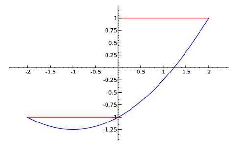
Figure 1.

Remark 3.

See the letter of Serre in the Appendix of [15] for previous examples showing how to use limited information towards the Sato-Tate conjecture to prove distribution results for Hecke eigenvalues (of a fixed modular form).

References

• [1] R. Bruggeman: Fourier coefficients of cusp forms, Invent. math. 45 (1978), 1–18.
• [2] B. Conrey, W. Duke and D. Farmer: The distribution of the eigenvalues of Hecke operators, Acta Arith. 78 (1997), 405–409.
• [3] J-M. Deshouillers and H. Iwaniec: Kloosterman sums and Fourier coefficients of cusp forms, Invent. math. 70 (1982), 220–288.
• [4] W. Duke and E. Kowalski: A problem of Linnik for elliptic curves and mean-value estimates for automorphic representations, with an Appendix by D. Ramakrishnan, Invent math. 139 (2000), 1–39.
• [5] H. Halberstam and H.E. Richert: Sieve methods, London Math. Soc. Monograph, Academic Press (London), 1974
• [6] H. Iwaniec, W. Kohnen and J. Sengupta: The first negative Hecke eigenvalue, International J. Number Theory 3 (2007), 355–363.
• [7] H. Iwaniec and E. Kowalski: Analytic number theory, AMS Colloquium Publ. 53, 2004.
• [8] E. Kowalski: The large sieve and its applications: arithmetic geometry, random walks and discrete groups, Cambridge Tracts in Math. 175, 2008.
• [9] Y.K. Lau and J. Wu: A large sieve inequality of Elliott-Montgomery-Vaughan type for automorphic forms and two applications, International Mathematics Research Notices, Vol. 2008, doi:10.1093/imrn/rmn162.
• [10] H-L. Montgomery: Topics in multiplicative number theory, Lecture Notes Math. 227, Springer-Verlag 1971.
• [11] H-L. Montgomery: The analytic principle of the large sieve, Bull. A.M.S. 84 (1978), 547–567.
• [12] E. Royer: Facteurs $\mathbf{Q}$-simples de $J_{0}(N)$ de grande dimension et de grand rang, Bull. Soc. Math. France 128 (2000), 219–248.
• [13] P. Sarnak: Statistical properties of eigenvalues of the Hecke operators, in “Analytic Number Theory and Diophantine Problems” (Stillwater, OK, 1984), Progr. Math. 70, Birkhäuser, 1987, 321–331.
• [14] J-P. Serre: Répartition asymptotique des valeurs propres de l’opérateur de Hecke $T_{p}$, J. American Math. Soc. 10 (1997), 75–102.
• [15] F. Shahidi: Symmetric power $L$-functions for $GL(2)$, in: “Elliptic curves and related topics”, edited by E. Kishilevsky and M. Ram Murty, CRM Proc. and Lecture Notes 4, 1994, 159–182.