F, G, K, M Spectral Standards in the $Y$ Band (0.95-1.11 $\mu$m)

Abstract

We take advantage of good atmospheric transparency and the availability of high quality instrumentation in the $1\,\micron$ near-infrared atmospheric window to present a grid of F, G, K, and M spectral standards observed at high spectral resolution ($R\approx$25,000). In addition to a spectral atlas, we present a catalog of atomic line absorption features in the $0.95-1.11\,\micron$ range. The catalog includes a wide range of line excitation potentials, from 0-13 eV, arising from neutral and singly ionized species, most frequently those of Fe i and Ti i at low excitation, Cr i, Fe i, and Si i at moderate excitation, and C i, S i, and Si i having relatively high excitation. The spectra also include several prominent molecular bands from CN and FeH. For the atomic species, we analyze trends in the excitation potential, line depth, and equivalent width across the grid of spectroscopic standards to identify temperature and surface gravity diagnostics near $1\,\micron$. We identify the line ratios that appear especially useful for spectral typing as those involving Ti i and C i or S i, which are temperature sensitive in opposite directions, and Sr ii, which is gravity sensitive at all spectral types. ASCII versions of all spectra are available in the online version of the journal.

1 Introduction

Since the advent of infrared arrays in the early 1990s, there have been many low resolution spectroscopic atlases published covering the $J$, $H$, or $K$ bands. Previous efforts that included the full O–M spectral classes and I–V luminosity classes made use of moderate resolution Fourier transform spectroscopy techniques (e.g., Wallace et al., 2000; Meyer et al., 1998; Wallace & Hinkle, 1997). An additional window of atmospheric transparency between these traditional near-infrared bands and the optical window, dubbed the $Y$ band, was highlighted by Hillenbrand et al. (2002). With existing observational capabilities on instruments at the IRTF, Keck, Las Campanas, and UKIRT telescopes, and with upcoming wide-field survey facilities such as Pan-STARRS and VISTA, the $Y$ band is becoming an increasingly appreciated and scientifically important near-infrared bandpass. Several low resolution ($R\equiv\lambda/\Delta\lambda\sim 2000$) spectral atlases for M, L, and T dwarfs have been published including $Y$ band data, e.g. Leggett et al. (1996), McLean et al. (2003), and Cushing et al. (2005). However, a high-resolution spectroscopic atlas covering earlier spectral types and the full range of luminosity classes has not yet appeared.

To complement existing moderate resolution catalogs in the $J$, $H$, and $K$ bands, we present here a high-resolution infrared spectral atlas for the $Y$ band. Our data cover the $0.94-1.12\,\mu$m region sampled by NIRSPEC (McLean et al., 1998) at the W. M. Keck Observatory. We obtained spectra of 20 MK-classified stars ranging in spectral type from F through M and in luminosity class from I–V for use as spectroscopic standards in future work. The data were processed as briefly described in Section 2. We present a representative grid of spectroscopic standards, a table of identified absorption features, and the resulting atlas of spectral lines in Section 3. In Section 4, we present relevant atomic data and illustrate as well as discuss line sensitivity to stellar effective temperature and surface gravity.

2 Target Selection, Data Acquisition, and Reduction

Near-infrared echelle spectra of 20 stars with well-established MK classifications were acquired between 2001 and 2009 with NIRSPEC (McLean et al., 1998, 2000) on Keck II. The targets, listed in Table 1, were drawn largely from the lists of standards utilized in the Meyer et al. (1998) and Wallace et al. (2000) studies of stellar photospheres in the $H$ and $J$ bands, while the remainder were selected by SIMBAD searches on spectral type and luminosity class, brightness, and accessibility. We used the N1 filter and have wavelength coverage from $0^{\prime\prime}.94$ to $1^{\prime\prime}.12$ $\mu$m at R = 25,000 ($\Delta$V = 12 km s^-1). The detector is a 1024 $\times$ 1024 pixel InSb chip, and the projected spectrograph slit we used was $0^{\prime\prime}.43\,\times\,12^{\prime\prime}$ in angular size. The $Y$ band is covered in 12 full and 2 partial orders, without gaps. The wavelength coverage of each order is given in Table 2.

Spectra were generally taken in nodded pairs using an ABBA pattern, with the astronomical target offset by $5^{\prime\prime}$ in each AB pair. Exposure times ranged from 1 to 720 s, integrated in the case of each spectral standard to acquire signal-to-noise ratios $\approx 100$ in the reduced one-dimensional spectra. Data reduction, including wavelength calibration and spatial rectification, extraction of one-dimensional spectra from the images, and removal of telluric emission and absorption features, is discussed in Edwards et al. (2006) and Fischer et al. (2008). We used a modified version of an IRAF script “reduceit” provided by Marianne Takamiya to reduce the 2002 and 2005 data, and we used the IDL package REDSPEC by S. Kim, L. Prato, and I. McLean to reduce data acquired in 2006 and 2009.

3 The Spectral Atlas

3.1 Illustration

From our 20 spectroscopic standards we identified a grid representing each of the four spectral classes (F, G, K, M) and three luminosity classes (I-I-I, III, IV–V; hereafter supergiants, giants, dwarfs). The star used to typify each class is indicated in Table 1 and was chosen based on having a good signal-to-noise ratio and relatively low rotational velocity ($v\,\sin(i)\lesssim 20\,\text{km s}^{-1}$). Figures 1a–1l show the grid of representative spectroscopic standards displayed from shorter to longer wavelengths for orders 80 through 69. Each spectrum is normalized to the local continuum and shifted to line rest velocity. Orders 81 and 68 at the edges of our wavelength coverage are excluded due to the low signal-to-noise ratio and the relatively high telluric contamination towards the edges of the $Y$ band window. As can be seen, the 1 $\mu$m spectral region is rich in spectral features. The absorption lines originate from both atomic and molecular species.

3.2 Line Identification

In order to generate a complete list of the atomic and molecular lines seen in the grid of spectroscopic standards, we began with a candidate list of transitions from the Infrared Atlas of the Arcturus Spectrum (Hinkle et al., 1995). Arcturus is a K2 III star and so its associated line list should be relevant for the majority of the cool stars in our sample, with some supplementing needed as described below—especially for the hotter stars. Of the 786 lines in our final candidate line list, 209 were added beyond those present in the Arcturus Atlas list. Because the Arcturus Atlas does not contain the complete details of each atomic transition (only line frequency and species), the candidate line list was cross-referenced with the Atomic Line Database (Kurucz et al., 1995) in order to obtain excitation potentials and log $gf$ values, as well as the Atomic Line List (van Hoof, 2009), to obtain the transition terms. The Kurucz line list was developed from theoretical computations and it is far more extensive in line transitions (over 16,000 within our wavelength range) than necessary given the moderate spectral resolution and signal-to-noise ratio typical of our (and most) empirical astrophysical data. Thus great care was taken to properly match the atomic data to the lines identified in the Arcturus Atlas. Each line in the Arcturus Atlas was matched by species, ionization, and wavelength within $\pm~{}10^{-5}\,\micron$ to lines in the Kurucz Atomic Line Database (in vacuum wavelengths). In some cases this resulted in multiple potential matches between the lists among lines of the same species but having different ionization states. Taking ionization into account generally resolved the situation but ambiguities often remained for lines such as the numerous Cr i, Fe i, and Ti i transitions. In such cases we chose to associate—at least initially—the Arcturus Atlas line with the Kurucz line possessing the largest log $gf$ among those with a realistic ($<$10 eV) lower excitation potential.

After the excitation potential, log $gf$, and transition term details of the atomic lines were added from the various sources to the candidate line list, the spectra were visually inspected. We observed that some lines identified in the Arcturus Atlas did not correspond to any observed spectral features. Lines that were not present at $\lesssim 1\%$ of the continuum level were flagged appropriately (as having strength 0 on the scale of 0–3 described below), as were any multiply matched to those in the Kurucz list but decided not to be the correct identification. These lines are ignored in our further analysis but remain in the candidate line list for reference.

Visual inspection of the spectra relative to the line list also identified strong absorption features seen in the spectra but not present in the assembled atomic line list. For later type stars (and especially prominent in the supergiants) such features were mostly identifiable as molecular lines based again on comparison to the Arcturus Atlas. We do not list these individually herein, but we found that nearly all unidentified strong lines in the later type stars appear to be molecular. For the earlier type F stars, additional atomic lines were identified using the Kurucz line list, now allowing for higher excitation potentials. In the case that there were multiple possible lines within the spectral resolution of the data ($0.4\,\text{\AA}$) the line with lowest ground state energy level was chosen. If this line was a species that had not been previously identified in the spectra, then other line candidates near the observed line center were considered.

After the initial matching using the Arcturus Atlas (Hinkle) and Atomic Line Database (Kurucz), all lines that were part of the same multiplet were identified using the on-line Atomic Line List (van Hoof). Any lines in multiplets of those already identified based on the above exercises and within the spectral range of the data were added to the line list if not already present, and are flagged as so in the final catalog. As above, we considered only the expected range of log $gf$ and excitation potential values when initially assigning new candidate lines based on multiplets. We then also considered the relative line strengths among the multiplets. Specifically, for optically thin (weak) lines in local thermodynamic equilibrium, the expected line intensity ratio $I_{1}/I_{2}$ is $A_{1}/A_{2}~{}g_{1}/g_{2}~{}\lambda_{2}/\lambda_{1}~{}e^{\Delta E/kT}$ or $I_{1}/I_{2}=g_{1}f_{1}/g_{2}f_{2}~{}\lambda_{2}^{3}/\lambda_{1}^{3}~{}e^{\Delta E/kT}$ where the symbols have their usual meanings. For stronger lines the line broadening factors should be taken into account but we have ignored this aspect for ease of analysis. In the case of multiplets (lines arising from the same lower level) the above expression simplifies because of the very small energy differences, to $I_{1}/I_{2}=(g_{1}f_{1}/g_{2}f_{2})(\lambda_{2}/\lambda_{1})^{3}$ which is what we use as a check on the line identifications. If during the multiplet analysis the case arose that an already-identified line could also be part of a multiplet from a different line species, we chose the multiplet identification over the alternative species unless both could be justified via multiplets or previous identification, in which case an additional flag for line blending was added.

We note that the line wavelengths as well as their other data as given among the Arcturus Atlas (Hinkle), the CfA Atomic Line Database (Kurucz) and the on-line Atomic Line List (van Hoof) were not always identical within quoted errors. Further, there are lines appearing in some of the above sources that are not available in the others. We believe sensible choices for line identifications have been made, and we have indicated remaining uncertainties in the tabulation. We also note that in some cases we have been unable to discern the transition term from the existing sources of atomic data. The 1 $\mu$m region is a relatively unscrutinized wavelength regime in stellar astrophysics and we are offering some of the first data that can help refine the available atomic line lists and parameters.

Finally, all lines in the catalog were assigned a numerical grade based on their relative strength in the spectroscopic standard grid. The grades range from zero to three, where the zero corresponds to lines that are not seen in any of the spectroscopic standards and are left in the catalog only for completeness, while the three is assigned to the deepest 2–10 lines per order (often deeper than 70% of the continuum level across multiple spectral types and luminosity classes). Throughout this paper, we consider a one to be a weak line (shallower than 90% of the continuum), while a two (deeper than 90% of continuum) or a three (up to 50% of continuum) is a strong line. Lines that were blended (at greater than the 50% level), or lines that were only seen in the F standards were also noted in the catalog. We note that for late-type and especially low-gravity stars, some expected atomic lines can be easily lost amidst strong molecular absorption features, generally CN lines which can exceed 80% depth in some orders. The number of lines in each strength classification, and the fractions that are molecular, blended, or only seen in the F standards are indicated in Table 3.

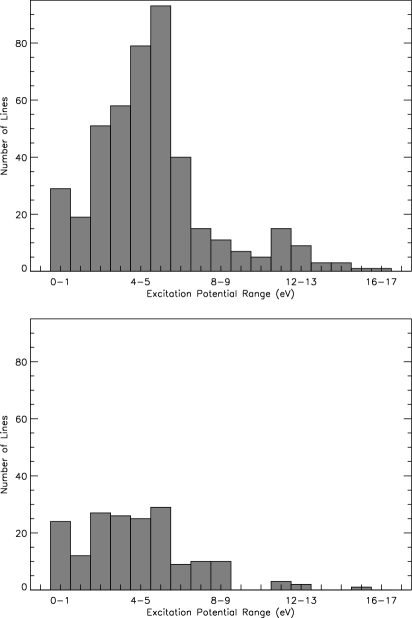
Figure 3: Distribution of excitation potentials for all 453 identified atomic transitions (top panel) and those 188 categorized as strong lines with line depth exceeding $90\%$ of the continuum level and appearing in Table 4 (bottom panel). The lines are divided into $1\,{\rm eV}$ bins according to the energy of the lower transition level. Most lines are in the $0-8\,{\rm eV}$ range, but there is a tail extending to higher excitation potential, up to $14\,{\rm eV}$. While the strong lines are more uniformly distributed in the peak excitation potential range, they are still representative of the whole of the line list.

The strongest (deepest) atomic and ionic lines, those given grades two and three above, plus their related atomic data are presented in Table 4. The log $gf$ values among this strong line set range from $-4.5$ and up for Fe i and Tii lines, to -2.5 and up for Cr i lines, to $-1.5$ and up for Si i lines, etc. We show in Figure 2 the lower excitation potential as a function of wavelength and of log $gf$ for these strong lines. The general trends in Figure 2 are as expected from atomic physics considerations. In Figure 3, we show a histogram of the number of atomic lines in 1 eV bins of the lower excitation levels, for both the entire line catalog and for just the strong lines (those presented in Table 4 and Figure 2). This figure is discussed in more detail below. The table and figures include only the 0.95–1.11 $\mu$m spectral region, where our final spectra are most uniform in signal-to-noise ratio across the standards grid.

4 Analysis

The strong atomic lines identified above as well as the molecular lines are illustrated in Figures 4a–5b using the extremes of our spectral type grid (F and M, giants and dwarfs) for comparison. Orders 79 and 71 appear to cover particularly useful spectral ranges for discriminating between hotter and cooler stars (see Section 4.2) based on the trade off in strong features as a function of spectral type.

Summarizing, notably present in the 1$\mu$m spectral region are numerous low and moderate excitation lines of neutral Ca i, Cr i, Fe i, K i, Mg i, Na i, Ni i, Si i, and Ti i along with singly ionized Sr ii. Lines of higher excitation potential like H i (and He i, though not within the effective temperature range sampled here), C i, N i, P i, and S i and singly ionized lines of Al ii, Ca ii, Fe ii, and Mg ii are also pervasive in the spectroscopic standards. Based on visual examination of the spectral grid, many of these lines are temperature sensitive and a few, such as Sr ii ($1.003940,\,1.033010,\,1.091790\,\micron$), are gravity sensitive. Such trends among the atomic lines are discussed more quantitatively below.

The spectra also feature many molecular lines, including (for all G–K–M types) a very prominent CN 0–0 transition molecular series with band heads near 1.093 $\mu$m ($R_{2}$) and 1.097 $\mu$m ($R_{1}$) according to McKellar (1988); these occur in the red part of order 70 and the series covers much of order 69. At the later spectral types (M stars), the FeH molecule has a prominent 0–0 band head (the “Wing–Ford” band which is apparent longward of $0.9896\,\micron$) and $Q$-branch (at $1.0061\,\micron$).

At even later spectral types, for which we do not have data, the $Y$ band contains TiO bands which appear at 0.942 and 0.950 $\mu$m, FeH appearing at 1.025 and 1.064 $\mu$m (Leggett et al., 1996), and VO appearing at 0.971 and 1.064 $\mu$m through $1.08\,\micron$ (Leggett et al., 1996; Cushing et al., 2003, 2005). There is also H₂O toward the short- and long-wavelength edges of the $Y$ band atmospheric window. Late M and L dwarfs also feature very prominent atomic K i, Na i, and Ca i features in the $Y$ band (Leggett et al., 1996; Lyubchik et al., 2004) that are only weakly (grade one on our system) or not present (grade zero) yet in the latest types among our spectra.

4.1 Trends in Excitation Potential

We examine in Figure 3 the distribution of energy levels for the suite of atomic spectral features identified in the $Y$ band (complete candidate line list as well as the strong lines of Table 4). The number of lines as a function of lower excitation potential is peaked at approximately 5 eV. The distribution declines more rapidly on the high excitation potential side of the peak than the lower, largely due to the presence of many strong moderate excitation Si i and Fe i transitions throughout the F, G, K, M spectral range. Heavier metals and higher ionization states generally contribute to the high excitation potential tail, while a large number of Ti i and some Cr i lines contribute to the lower excitation potential tail. Notable exceptions to this general trend include several C i lines at $\sim 7-10$ eV, and a few H i lines in the upper excitation potential range. As expected, many of these high excitation potential lines are only seen (with strength values of 3 or 2 on our system) among the earlier type F stars within our spectroscopic grid.

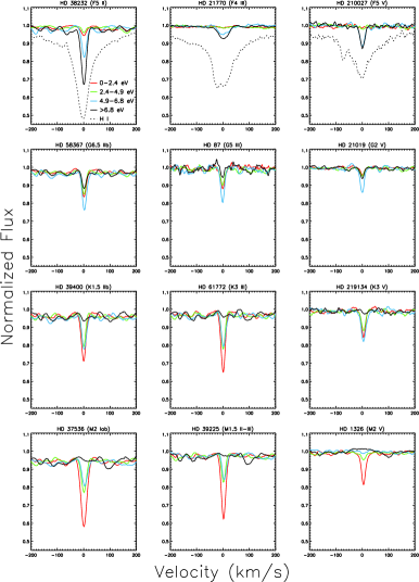
Figure 6: Average profiles of strong lines in four different excitation potential ranges: 0–2.4 eV (red; containing 35 lines), 2.4–4.9 eV (green; containing 41 lines), 4.9–6.8 eV (blue; containing 29 lines), and $>6.8\,{\rm eV}$ (black; containing 26 lines). The three H lines are excluded from the calculation of the solid black profile but are shown separately for the F stars as the dotted black line (in the cooler standards the H profile is too heavily blended with neighboring features for the absorption profile to be informative). Only lines that are unblended and strong enough to be tabulated in Table  4 are included. A clear trend can be seen with hotter stars having stronger high-excitation lines compared to cooler stars having stronger low-excitation lines. Additionally, supergiants tend to have stronger lines then the dwarfs in the same spectral class.

In Figure 6, we have plotted for the spectroscopic standards grid the average line profile for four different bins in excitation potential. The atomic lines were divided into bins such that roughly the same number of $Y$ band lines are contained in each bin, but with an attempt to minimize the splitting of lines of the same species into multiple bins. This resulted in divisions at $2.4$, $4.9$, and $6.8\,{\rm eV}$. Only strong, unblended lines were included. However, hydrogen lines as well as any lines within $\pm 0.0005\,\micron$ of it were excluded since these particularly strong/broad lines dominate in the averaged profiles over nearby line features. There are 35 lines in the 0-2.4 eV bin, 41 lines in the 2.4–4.9 eV bin, 29 lines in the 4.9–6.8 eV bin, and 26 lines in the $>6.8$ eV bin.

As expected, the hotter stars tend to have stronger lines with higher excitation potentials while cooler stars are dominated by low excitation potential lines. Supergiants also tend to have stronger lines overall relative to the dwarfs. Specifically, the F stars are dominated by the 6.8 eVand higher lines, the G stars are dominated by the 4.9–6.8 eV lines, and the M stars are dominated by the 0–2.4 eV lines. One would expect that the K stars would lie in sequence and be dominated by the 2.4–4.9 eV lines. Instead, we find that the line strengths are roughly constant from 0 to 6.8 eV and comparable to the 4.9–6.8 eV bin in the G standards. Although the K standards do fit within the overall excitation-potential-temperature trend, they do not match the observed pattern in detail in the expected way.

4.2 Diagnostic Lines for Spectral Classification

Among the strong lines there are some obvious temperature dependencies apparent in Figures 4a-5b. For example, in order 79, there are several strong C i lines that appear in the early spectral types and are not seen in the later types. In the same order there are also Ti i lines that complement this trend, appearing very strongly in the late spectral types, but only weakly, if at all, in the early spectral types. A similar trend can be seen in order 73 for Si i relative to Ti i, and in order 71 for both C i and Si i relative to Ti i.

We investigated through equivalent width analysis the behaviors with both effective temperature and surface gravity of the various strong lines in the 1 $\mu$m region. Several strong lines stand out over the others in Table 4 as potentially useful for analytic or diagnostic purposes, the strongest of which have line depths greater than 50% of the continuum level. Figure 7 plots the equivalent widths of several such lines versus the standard star effective temperature. In constructing this plot we were particularly sensitive to including those lines with temperature dependencies discernable for dwarf stars. As discussed above, lines of note include C i and S i multiplets, which show a strong temperature dependence, and several Ti i multiplets, which show a strong inverse temperature dependence. This behavior was also highlighted by Lyubchik et al. (2004) for the a5F–z5Go multiplet of Ti i in the 1.04-1.07 $\mu$m region, though we find many of these long wavelength lines of the multiplet blended with other strong lines. Ca i, Cr i, and Fe i have generally weaker (inverse) temperature dependence. Several neutral H i lines and higher excitation potential neutral metals such as C i, P i, and S i and the singly ionized metals Ca ii, Fe ii, and Mg ii appear only in the F standards and are therefore also good temperature indicators. The Si i lines peak in strength in the G–K spectral range and become weaker toward both F and M types, with some gravity sensitivity. In addition to their temperature dependence, the Ti i lines are also gravity sensitive at log $T_{\rm eff}<$ 3.7 as are the C i and S i lines at log $T_{\rm eff}\,>3.7$. Sr ii shows gravity dependence at all temperatures but little trend with temperature.

We have identified a few lines having line depth ratio that are useful indicators of spectral and luminosity class. These ratios versus standard star effective temperature are illustrated in Figure 8. The Ti i ($1.049900\,\micron$) and Sr ii ($1.033010\,\micron$) lines, are the temperature and gravity sensitive lines, respectively, with the strongest trends apparent in Figure 7. In this case, division of the temperature-sensitive line by the gravity-sensitive line spreads the spectroscopic standards such that dwarfs and then giants have increased line strength relative to supergiants at similar effective temperatures. The Ti i ($1.049900\,\micron$) and C i ($1.068830\,\micron$) lines are both temperature sensitive, but the temperature dependence of C i is opposite that of Ti i. This creates an amplified trend in line strength versus temperature relative to that of the single lines (as in Figure 7). We also investigated lines pairs that were closer together in wavelength and therefore suitable for temperature and gravity designation from single-order moderate to high dispersion spectra. Thus the Ca i ($1.034670\,\mu{\rm m}$) $/$ Sr ii ($1.033010\,\mu{\rm m}$) ratio is also illustrated as sensitive to gravity and the Ti i ($1.068000\,\mu{\rm m}$) $/$ C i ($1.071030\,\mu{\rm m}$) ratio as sensitive to temperature. Either of these line pair sets could be used in comparing the relative spectral typing of a set of previously unclassified stellar spectra, depending on the spectral dispersion

Although not present in our effective temperature range, there is a high excitation (21 eV) He i line at $1.08333\,\micron$ in addition to the high excitation potential (12 eV) H i lines already noted here. These He i and H i lines are useful spectral type diagnostics for O, B, and A stars. Both lines are also particularly sensitive probes at all spectral types of energetic circumstellar processes such as chromospheric activity and wind processes (Edwards et al., 2006; Fischer et al., 2008).

5 Summary

We have presented a spectral atlas for the $Y$ band region of the near infrared portion of the electromagnetic spectrum. Our data set consists of a grid of MK-classified stars for use as spectroscopic standards spanning the F through M spectral classes and I–V luminosity classes observed at R$\approx$25,000. The associated catalog of identified lines contains numerous spectral absorption features, both atomic and molecular in origin, that span a wide range of excitation potentials. Many of the atomic features show strong line depth and equivalent width trends across the spectral atlas. This atlas and the identified atomic spectral lines are potentially useful for two-dimensional spectral classification, especially line depth ratios involving Ti i and C i or S i, which are temperature sensitive in opposite directions, and Sr ii, which is gravity sensitive. ASCII versions of all spectra are available to download with the online version of the journal (an example of the form and content of these spectra can be found in Table 5).

Table 1: Spectral Reference Stars

(1)	(2)	(3)	(4)	(5)	(6)	(7)
Name	Alt. Name	Obs. Date	Sp. Type	$T_{eff}$ [K]	Sp. Type Reference	Template
HD 21770	HR 1069	2006 Nov 30	F4 III	7170	Roman (1952)	X
HD 193370	HR 7770	2006 Nov 30	F5 Ib	6640	Griffin & Redman (1960)
HD 38232	BD+29 983	2005 Dec 13	F5 II	6640	Bidelman (1957)	X
HD 55052	HR 2706	2002 Nov 26	F5 III	6470	Harlan (1969)
HD 210027	HR 8430	2006 Nov 30	F5 V	6530	Morgan et al. (1943)	X
HD21019	HR 1024	2006 Nov 29	G2 V	5830	Harlan (1974)	X
HD 87	HR 4	2009 Jul 11	G5 III	5072	Barnes et al. (1986)	X
HD 58367	HR 2828	2005 Dec 13	G6 IIb	4720	Keenan & McNeil (1989)	X
HD 75935	BD+27 1682	2006 Nov 30	G8 V	5430	Montes et al. (2001)
HD 166	HR 8	2006 Nov 30	K0 V	5240	Basri & Batalha (1990)
HD 39400	HR 2037	2005 Dec 13	K2 IIb	4330	Keenan & McNeil (1989)	X
BD +59 2667	$\cdots$	2006 Nov 30	K2 IV	5010	Basri & Batalha (1990)
HD 61772	HR 2959	2005 Dec 13	K3 III	4320	Houk & Smith-Moore (1988)	X
HD 219134	HR 8832	2006 Nov 30	K3 V	4780	Morgan et al. (1943)	X
HD 201091	61 CygA	2006 Dec 01	K5 V	4340	Morgan et al. (1943)
HD 201092	61 CygB	2006 Dec 01	K7 V	4040	Griffin & Redman (1960)
HD 232979	BD+52 857	2006 Nov 30	M0.5 V	5240	Keenan & McNeil (1989)
HD 39225	HR 2028	2005 Dec 13	M1+ III	3550	Keenan & McNeil (1989)	X
HD 37536	HR 1939	2005 Dec 13	M2 Iab	3450	Sharpless (1966)	X
HD 1326	Gl 15A	2006 Nov 30	M2 V	3530	Keenan & McNeil (1989)	X

Table 2: Effective Wavelength Coverage

(1)	(2)
Order	$\lambda$ Range [$\mu$m]
81	0.94118 - 0.94813
80	0.94646 - 0.95985
79	0.95835 - 0.97192
78	0.97054 - 0.98543
77	0.98304 - 0.99696
76	0.99590 - 1.00998
75	1.00906 - 1.02332
74	1.02255 - 1.03709
73	1.03628 - 1.05122
72	1.05081 - 1.06578
71	1.06553 - 1.08065
70	1.08065 - 1.09604
69	1.09584 - 1.11184
68	1.11241 - 1.12224

Table 3: Distribution of Line Strengths

(1)	(2)	(3)		(4)		(5)
Strength Class	Line Depth	No. Lines		No. in F Stars Only		No. in Blends
		Atomic	Molecular	Atomic	Molecular	Atomic	Molecular
0	Unobserved	99	$\cdots$	$\cdots$	$\cdots$	$\cdots$	$\cdots$
1	$>90\%$	237	279	20	0	2	0
2	$<90\%$, $\gtrsim 70\%$	141	50	18	0	11	22
3	$\lesssim 70\%$	75	4	14	0	10	0

.

Table 4: Identified Atomic Spectral Lines

(1)	(2)	(3)	(4)	(5)	(6)	(7)	(8)
Wavelength[$\micron$]	Atom/Ion	log $gf$	$E_{lower}$ [eV]	$E_{upper}$ [eV]	Term	Strength	Comment
0.9504665	Mn i	-1.200	5.69633	7.00088	??	2B	Uncertain but in the Arcturus list
0.950867	Ti i	0.078	3.58290	4.88689	y5Fo-f5F	2B
0.951329	Ti i	-0.316	3.55869	4.86196	y5Fo-f5F	2B
0.951587	Fe i	-1.491	5.03341	6.33641	x5Fo-f5F	2
0.952265	N ii	-0.960	4.16750	5.46958	y3Do-e3D	2
0.954859	H i	-0.540	12.08751	13.38597	3-8	3F
0.954865	Ti i	-1.598	0.83605	2.13459	a5F-z5Fo	3	*
0.957253	Fe i	-0.542	4.99161	6.28690	x5Fo-e5G	2
0.957438	Cr i	-1.784	2.54444	3.83949	a5G-z5Fo	2B
0.957692	Cr i	-1.088	2.54479	3.83949	a5G-z5Fo	3B
0.960218	Ti i	-1.440	0.82591	2.11721	a5F-z5Fo	3	*
0.960567	C i	-0.940	7.48090	8.77172	3Po-3S	3F
0.962342	C i	-0.516	7.48278	8.77114	3Po-3S	3F
0.962903	Cr i	-3.451	2.91531	4.20301	a3P-z3Po	2B
0.962913	Fe i	-0.610	5.03340	6.32108	x5Fo-e5G	2
0.963682	Fe i	-0.607	5.06412	6.35078	x5Fo-e5G	2
0.964090	Ti i	-0.638	0.84848	2.13459	a5F-z5Fo	3B	Only weak blend, *
0.965002	Ti i	-1.462	0.81820	2.10309	a5F-z5Fo	3	*
0.965222	S i	0.350	8.41201	9.69661	3Do-3D	2F
0.965576	Fe i	-0.778	4.73346	6.01759	y3Do-e3F	2
0.966108	C i	-0.264	7.48830	8.77172	3Po-3S	3F
0.967314	Cr i	-1.230	2.54400	3.82626	a5G-z5Fo	2
0.967494	S i	-0.090	8.40872	9.69031	3Do-3D	2F
0.967815	Ti i	-0.831	0.83605	2.11721	a5F-z5Fo	3	*
0.968346	S i	0.100	8.40982	9.69028	3Do-3D	2F
0.969133	Ca i	-0.422	4.73889	6.01830	3Do-3P	2B
0.969146	Ti i	-1.638	0.81300	2.09240	a5F-z5Fo	3	*
0.969651	Fe i]	-3.115	5.08593	6.36467	x5Fo-e7F	2B
0.970242	Fe i]	-2.215	5.06412	6.34208	x5Fo-e7F	2
0.970459	Ca i	-0.169	4.74385	6.02151	3Do-3P	2
0.970834	Ti i	-1.037	0.82591	2.10309	a5F-z5Fo	3	*
0.971964	Ti i	-1.590	2.30552	3.58121	z5Do-a5D	2
0.972167	Ti i	-1.272	1.50259	2.77801	a1G-z1Fo	2
0.973100	Ti i	-1.234	0.81820	2.09240	a5F-z5Fo	3	*
0.973719	Cr i	-1.377	2.54400	3.81740	a5G-z5Fo	2
0.974037	Ti i	-1.882	2.29697	3.56995	z5Do-a5D	2B
0.974124	Fe i	0.037	4.99161	6.26447	x5Fo-e5G	2B
0.974625	Ti i	-1.334	0.81300	2.08521	a5F-z5Fo	3	*
0.974956	Ti i	-1.258	2.31807	3.58984	z5Do-a5D	2B
0.976610	Fe i	-0.468	5.09989	6.36951	x5Fo-e5G	2B
0.976658	Fe i]	-1.123	5.03341	6.30297	x5Fo-e7F	2B
0.977293	Ti i	-1.604	0.84848	2.11721	a5F-z5Fo	3
0.978602	Ti i	-1.452	0.83605	2.10309	a5F-z5Fo	3	* As blend
0.978623	Ti i	-1.643	0.81820	2.08521	a5F-z5Fo	3	* As blend
0.979030	Ti i	-1.469	0.82591	2.09240	a5F-z5Fo	3	* Blend
0.980352	Fe i]	-2.223	5.09989	6.36467	x5Fo-e7F	2
0.985746	Ca ii	-0.228	7.505644	8.763499	2Po-2S	2F
0.986444	Fe i	-0.299	5.06412	6.32109	x5Fo-e5G	2F
0.989175	Fe i	-0.125	5.03341	6.28690	x5Fo-e5G	2
0.989334	Ca ii	-0.601	8.438551	9.69184	2Fo-2G	3F
0.992711	Fe i]	-3.095	3.54676	4.79579	a1D-y3Do	2
0.993006	Ti i	-1.580	1.87933	3.12799	a3G-y3Fo	2
0.993410	Ca ii	0.072	7.515348	8.763499	2Po-2S	2F
0.994412	Ti i	-1.924	2.16043	3.40732	a3D-x3Do	2
0.995181	Ti i	-1.831	2.15370	3.39963	a3D-x3Do	2B
0.996401	Na i	-0.820	3.61721	4.86162	2D-2Fo	2B	Doublet, ${\dagger}$
1.000032	Fe ii	-1.826	5.48450	6.72439	z4Fo-b4G	2F
1.000070	Ti i	-1.840	1.87329	3.11313	a3G-y3Fo	2B
1.000580	Ti i	-1.135	2.16043	3.39963	a3D-x3Do	2
1.001460	Ti i	-1.258	2.15370	3.39182	a3D-x3Do	2
1.003720	Ti i	-2.002	1.46024	2.69556	b3F-z3Go	3
1.003940	Sr ii	-1.312	1.80482	3.03988	2D-2Po	3
1.005160	Ti i	-2.131	1.44325	2.67681	b3F-z3Go	3
1.005210	H i	-0.303	12.08830	13.32180	3-7	3F
1.006050	Ti i	-0.900	2.17485	3.40732	a3D-x3Do	2
1.006270	Ti i	-2.278	1.42985	2.66206	b3F-z3Go	2
1.006780	Fe i	-2.098	4.83518	6.06676	y3Do-e3F	2
1.009498	Mg ii	1.020	11.63047	12.85873	2Fo-2G	2F
1.0115253	N i	0.595	11.75833	12.98412	4Do-4F	2F
1.011680	Fe i	-3.771	2.75876	3.98438	a3G-z3Fo	2
1.0117413	N i	0.755	11.76464	12.990176	4Do-4F	2F
1.012370	Ti i	-1.672	2.17485	3.39963	a3D-x3Do	2B
1.012660	C i	-0.032	8.53767	9.76209	1P-1Po	3F
1.014830	Fe i	-0.298	4.79579	6.01759	y3Do-e3F	2
1.015790	Fe i	-4.229	2.17609	3.39674	a5P-z5Fo	2
1.017030	Fe i	-4.061	2.19801	3.41718	a5P-z5Fo	2
1.017326	Ti i	-3.292	1.44325	2.66206	b3F-z3Go	2
1.019192	Ti i	-3.264	1.46024	2.67681	b3F-z3Go	2
1.019600	N ii	-0.790	4.08956	5.30564	1Po-5/2[5/2]	2
1.019790	Fe i	-3.699	2.72773	3.94359	a3G-z3Fo	2
1.021910	Fe i	-0.215	4.73346	5.94680	y3Do-e3F	2	*
1.022120	Fe i	-2.760	3.07155	4.28464	c3P-z3Po	2
1.026800	Fe i	-4.467	2.22286	3.43042	a5P-z5Fo	2B
1.029180	Si i	-1.360	4.92042	6.12519	3Po-3S	2B
1.033010	Sr ii	-0.353	1.83958	3.03988	2D-2Po	3	*
1.033310	N ii	-1.228	4.10569	5.30564	3Go-3F	2
1.034370	Fe i	-3.493	2.19801	3.39674	a5P-z5Fo	3	* As blend
1.034670	Ca i	-0.408	2.93271	4.13109	1Po-1S	3	* As blend, ${\dagger}$
1.037411	SiI	-0.447	4.92965	6.12519	3Po-3S	2	*
1.038150	N ii	-0.965	4.08846	5.28282	?	2B
1.038184	Fe i	-4.065	2.22286	3.41718	a5P-z5Fo	2B
1.039860	Fe i	-3.330	2.17609	3.36848	a5P-z5Fo	3B	* As blend
1.039961	Ti i	-1.537	0.84848	2.04076	a5F-z5Go	3B	* As blend
1.042590	Fe i	-3.776	2.69259	3.88187	a3G-z3Fo	2B
1.042660	Fe i	-2.916	3.07155	4.26074	c3P-z3Po	2B	*
1.045544	[Fe i]	?	0.99	2.17	a3F-a5P	2	In Arcturus list
1.045830	S i	0.260	6.86061	8.04620	3So-3P	3F
1.045960	S i	-0.430	6.86061	8.04605	3So-3P	2F
1.046230	S i	0.040	6.86061	8.04575	3So-3P	3F
1.047250	Fe i	-1.229	3.88377	5.06775	z3Do-3P	2	*
1.048910	Cr i	-0.972	3.01083	4.19294	b5Dz5Do	2
1.049900	Ti i	-1.651	0.83605	2.01705	a5F-z5Go	3
1.050438	Fe ii	-1.997	5.54914	6.72953	z4Fo-b4G	2F
1.051290	Cr i	-1.558	3.01351	4.19294	b5Dz5Do	2
1.05324	P i	0.200	6.95482	8.13207	4P-4Do	2F
1.053340	N ii	-1.189	4.10569	5.28282	??	2
1.053510	Fe i	-1.532	3.92887	5.10582	z3Do-3P	2
1.054410	C i	-1.290	8.53767	9.71361	1P-1Po	2F
1.058000	Fe i	-3.268	3.30163	4.47357	b3H-z3Go	2
1.058450	P i	0.480	6.98570	8.15716	4P-4Do	2F
1.058750	Ti i	-1.777	0.82591	1.99703	a5F-z5Go	3B	* As blend
1.058800	Si i	-0.020	4.95413	6.12519	3Po-3S	3B	* As blend, ${\dagger}$
1.060630	Si i	-0.380	4.92998	6.09902	3Po-3P	3	* As blend, ${\dagger}$
1.061060	Ti i	-2.676	0.84848	2.01705	a5F-z5Go	3	* As blend
1.06146	Fe i	-0.336	6.16964	7.33777	n7Fo-9/2[13/2]	2
1.06196	Fe i	-3.257	3.26733	4.43491	b3H-z3Go	2
1.063060	Si i]	0.000	5.86287	7.02925	1P-3Po	2
1.063883	Al ii	-0.610	15.30358	16.46905	3Fo-3D	2F
1.065050	Cr i	-1.613	3.01083	4.17502	b5Dz5Do	2
1.066390	Si i	-0.350	4.92042	6.08315	3Po-3P	3B	* As blend, ${\dagger}$
1.066460	Ti i	-1.916	0.81820	1.98085	a5F-z5Go	3B	* As blend
1.067047	Cr i	-1.489	3.01301	4.17502	b5Dz5Do	2
1.067510	Cr i	-1.374	3.01351	4.17502	b5Dz5Do	2
1.068000	Ti i	-2.507	0.83605	1.99703	a5F-z5Go	3
1.068600	C i	0.076	7.48328	8.64360	3Po-3D	3F
1.068830	C i	-0.276	7.48090	8.64098	3Po-3D	3F
1.069260	Si i	-0.190	5.95413	7.11374	3D-3Fo	2	*
1.069420	C i	0.348	7.48830	8.64774	3Po-3D	3F
1.069720	Si i	-0.060	5.96433	7.12345	3D-3Fo	2
1.071030	C i	-0.401	7.48328	8.64098	3Po-3D	3F
1.072920	Ti i	-2.064	0.81300	1.98652	a5F-z5Go	3B
1.073030	Si i	0.060	5.98441	7.13995	3D-3Fo	3B
1.073250	C i	-0.401	7.48830	8.64360	3Po-3D	3F
1.073590	Ti i	-2.504	0.82591	1.98085	a5F-z5Go	3
1.075230	Si i	-0.300	4.92998	6.08315	3Po-3P	3
1.075595	Fe i	-1.902	3.95999	5.11277	z3Do-3P	2
1.075690	C i	-1.590	7.48830	8.64098	3Po-3D	2F
1.077770	Ti i	-2.658	0.81814	1.96852	a5F-z5Go	3
1.07836	Fe i	-3.414	3.23694	4.38676	b3H-z3Go	2
1.078600	Fe i	-2.597	3.11117	4.26074	c3P-z3Po	2
1.078751	Si i	-0.910	5.96433	7.11374	3D-3Fo	2
1.078980	Si i	-0.390	4.92998	6.07914	3Po-3P	3
1.08043	Cr i	-1.715	3.01135	4.15897	b5D-z5Do	2
1.081410	Mg i	-0.320	5.94632	7.09290	3D-3Fo	2B	${\dagger}$
1.082130	Fe i	-1.998	3.95999	5.10582	z3Do-3P	2B
1.082470	Cr i	-1.678	3.01351	4.15897	b5D-z5Do	2
1.083010	Si i	0.220	4.95413	6.09902	3Po-3P	3
1.083091	Ti i	-3.878	0.83605	1.98085	a5F-z5Go	2B
1.08378	Na i	-0.500	3.61721	4.76129	2D-2Fo	2	${\dagger}$
1.084680	Si i	-0.310	5.86287	7.00599	1P-1Do	2
1.086562	Fe ii	-2.121	5.58957	6.73071	z4Fo-b4G	2F
1.086650	Fe i]	-0.803	4.73346	5.87452	y3Do-e5F	2
1.087180	Si i	0.040	6.19142	7.33192	3Fo-3/2[9/2]	2B
1.087250	Si i	0.320	5.08269	6.22311	1Po-1D	3B	${\dagger}$
1.08847	Fe i]	-3.713	2.84523	3.98438	b3P-z3Fo	2
1.088578	Si i	-0.870	5.98441	7.12345	3D-3Fo	2
1.08883	Si i	0.040	6.18113	7.31990	3Fo-3/2[7/2]	2
1.089930	Fe i	-2.729	3.07155	4.20917	c3P-z3Po	2
1.090886	Cr i	-0.647	3.43820	4.57480	y7Po-e7S	2
1.091723	Mg ii	0.020	8.86425	10.00002	2D-2Po	2FB
1.091790	Sr ii	-0.638	1.80482	2.94051	2D-2Po	3
1.091827	Mg ii	-0.930	8.86436	10.00002	2D-2Po	2FB
1.093287	Cr i	-2.330	3.01351	4.15897	b5D-z5Do	2	Amidst CN bands
1.094110	H i	0.002	12.08830	13.22160	3-6	3F
1.095477	Mg ii	-0.230	8.86436	9.99622	2D-2Po	2F
1.095630	Mg i	-0.852	5.93194	7.06364	3Po-3D	2B	${\dagger}$
1.096023	Cr i	-2.067	3.01351	4.15897	b5D-z5Do	2B
1.096030	Mg i	-0.690	5.93235	7.06364	3Po-3D	2B	${\dagger}$
1.096845	Mg i	-0.250	5.93319	7.06363	3Po-3D	2B	CN band head confused, ${\dagger}$
1.097038	P i	0.120	8.07889	9.20914	2D-2Do	2F
1.098231	SiI	-0.590	4.95413	6.08315	3Po-3P	3
1.098284	N ii	-0.929	4.15386	5.28282	y3Do-e3D	3F
1.09851	Si i	-0.050	6.19142	7.32015	3Fo-3/2[7/2]	2
1.09875	Si i	-0.500	6.19142	7.31990	3Fo-3/2[7/2]	2
1.10163	Fe i]	-1.334	4.79579	5.92133	y3Do-e5F	2B
1.101870	Cr i	-0.515	3.43820	4.57480	y7Po-e7S	2
1.102100	Si i	0.610	6.20642	7.33148	3Fo-3/2[9/2]	3
1.102287	KI	-0.010	2.67014	3.79501	2D-2Fo	2	Doublet, wavelength off, ${\dagger}$
1.104770	Cr i	-2.508	3.01135	4.13369	b5D-z5Do	2

Note. — This subset of the lines in our assembled line list includes those lines seen among the standards grid that are rated at 3 or 2 in strength (i.e., absorption below 90% of the continuum level). Not tabulated are lines from our list rated 1 (weaker absorption than 90% of the continuum) or 0 (not present at our spectral resolution or a likely misidentification) in strength. Wavelengths are those in vacuum. In addition to the line strength, the “Strength” column also indicates which lines are blended at greater than the 50% level (marked with a B) and which lines that are only seen in the F spectroscopic standards (marked with an F). The “Comments” column indicates lines seen in the lower resolution $R=2000$ $Y$ band data of Cushing et al. (2005) (marked with an asterisk), lines identified as possibly present in the $R=250$ data of Leggett et al. (1996) (marked with a dagger), or other information.

Table 5: Sample Normalized Spectrum of HD 87, Order 69

(1)	(2)
$\lambda$ [$\mu$m]	Normalized Flux
1.0963141	1.07008
1.0963299	1.07359
1.0963458	1.10119
1.0963615	1.08921
1.0963775	1.11744
1.0963933	1.14190
1.0964092	1.08628
1.0964249	1.06581
1.0964408	1.08024
1.0964566	1.03010

Note. — In this table, we present a sample demonstrating the form and content of the spectra available for download with the online edition of the journal. Similar spectra are available in the online journal (spectra.tar.gz).

Figure 1a: Order 80 for the grid of spectroscopic standards. The four rows from top to bottom are the F, G, K, and M standards, and the three columns from left to right are the supergiants (I–II), giants (III), and dwarfs (IV–V). Each NIRSPEC spectral order is represented in a subsequent figure. (b) Same as (a), order 79. (c) Same as (a), order 78. (d) Same as (a), order 77. (e) Same as (a), order 76. (f) Same as (a), order 75. (g) Same as (a), order 74. (h) Same as (a), order 73. (i) Same as (a), order 72. (j) Same as (a), order 71. (k) Same as (a), order 70. (l) Same as (a), order 69.

Figure 1b: (Continued)

Figure 1c: (Continued)

Figure 1d: (Continued)

Figure 1e: (Continued)

Figure 1f: (Continued)

Figure 1g: (Continued)

Figure 1h: (Continued)

Figure 1i: (Continued)

Figure 1j: (Continued)

Figure 1k: (Continued)

Figure 1l: (Continued)

Figure 2: Lower excitation potential as a function of wavelength (left) and log $gf$ (right) for atomic lines identified in Table 4.

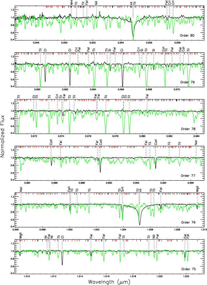
Figure 4a: Strong atomic lines tabulated in Table  4 (vertical dotted lines with element names) identified relative to the supergiant spectroscopic standards HD 38232, an F5 ii (black line) and HD 37536, an M2 Iab (green line). Weaker atomic lines from our completed catalog are marked at the top (short black hashes) as are molecular lines (short red hashes) (A color version of this figure is available in the online journal.).

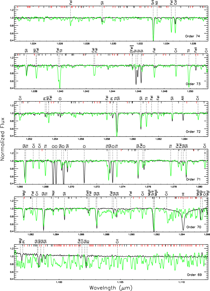
Figure 4b: (Continued)

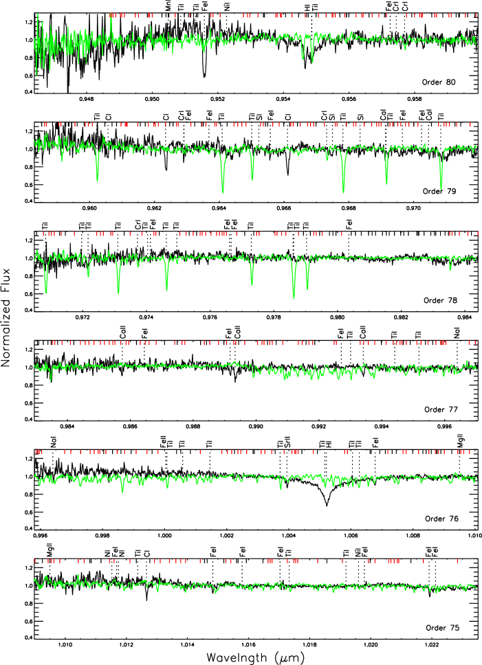
Figure 5a: Strong atomic lines tabulated in Table  4 (vertical dotted lines with element names) identified relative to the dwarf spectroscopic standards HD 55052, an F5 V (black line) and HD 1326, an M2 V (green line). Weaker atomic lines from our completed catalog are marked at the top (short black hashes) as are molecular lines (short red hashes) (A color version of this figure is available in the online journal.).

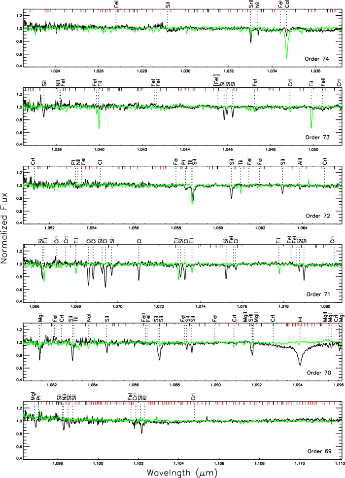
Figure 5b: (Continued)

Figure 7: Equivalent widths in angstroms of diagnostically useful lines vs. the effective temperature of the spectroscopic standards. Squares represent supergiants, triangles the giants, and crosses the dwarf standards. Lines connect the existing data and should not be misinterpreted as defining the detailed trend with temperature. Lines were chosen from Table 4 as those of strength three with significant temperature and/or gravity sensitivity within our spectral grid. Generally, only one line from among those in a multiplet set is shown; its behavior is typical of all lines in the multiplet. The three columns depict lines with higher excitation potential (left), lines with lower excitation potential (right), and lines sensitive to surface gravity (center). Within each column the panels are ordered from top to bottom alphabetically by line species and then by increasing wavelength.

Figure 8: Top panels: the ratio of line strengths for a temperature-sensitive and a gravity-sensitive line, as a function of the stellar effective temperature. The left side shows Ti i ($1.049900\,\mu{\rm m}$) $/$ Sr ii ($1.033010\,\mu{\rm m}$), the lines with the strongest temperature and gravity trends in our spectra, while the right side shows Ca i ($1.034670\,\mu{\rm m}$) $/$ Sr ii ($1.033010\,\mu{\rm m}$) which are chosen due to their proximity in wavelength. Bottom panel: the ratio of line strengths for two temperature sensitive lines with opposite temperature dependence, Ti i ($1.049900\,\mu{\rm m}$) and C i ($1.068830\,\mu{\rm m}$) on the left side and Ti i ($1.068000\,\mu{\rm m}$) and C i ($1.071030\,\mu{\rm m}$) on the right side, as a function of stellar effective temperature. Squares represent supergiants, triangles the giants, and crosses the dwarf standards. Although strong dependences are evident, the illustrated lines connect the existing data only and should not be misinterpreted as defining the detailed trends with temperature.

References

- Barnes et al. (1986) Barnes, III, T. G., Moffett, T. J., & Slovak, M. H. 1986, PASP, 98, 223
- Basri & Batalha (1990) Basri, G. & Batalha, C. 1990, ApJ, 363, 654
- Bidelman (1957) Bidelman, W. P. 1957, PASP, 69, 147
- Cushing et al. (2003) Cushing, M. C., Rayner, J. T., Davis, S. P., & Vacca, W. D. 2003, ApJ, 582 1066
- Cushing et al. (2005) Cushing, M. C., Rayner, J. T., & Vacca, W. D. 2005, ApJ, 623, 1115
- Edwards et al. (2006) Edwards, S., Fischer, W., Hillenbrand, L., & Kwan, J. 2006, ApJ, 646, 319
- Fischer et al. (2008) Fischer, W., Kwan, J., Edwards, S., & Hillenbrand, L. 2008, ApJ, 687, 1117
- Griffin & Redman (1960) Griffin, R. F. & Redman, R. O. 1960, MNRAS, 120, 287
- Harlan (1969) Harlan, E. A. 1969, AJ, 74, 916
- Harlan (1974) Harlan, E. A. 1974, AJ, 79, 682
- Hillenbrand et al. (2002) Hillenbrand, L. A., Foster, J. B., Persson, S. E., & Matthews, K. 2002, PASP,114,708
- Hinkle et al. (1995) Hinkle, K., Wallace, L., & Livingston, W. 1995, PASP, 107,142
- Houk & Smith-Moore (1988) Houk, N., & Smith-Moore, M. 1988, Michigan Catalogue of Two-Dimensional Spectral Types for the HD Stars, Vol. 4 (Ann Arbor: Univ. Michigan)
- Keenan & McNeil (1989) Keenan, P. C. & McNeil, R. C. 1989, ApJS, 71, 245
- Kurucz et al. (1995) Kurucz, R.L. & Bell, B. 1995, Atomic Line Data, Kurucz CD-ROM No. 23, Cambridge, MA: Smithsonian Astrophysical Observatory.
- Leggett et al. (1996) Leggett, S.K., Allard, F., Berriman, G., Dahn, C.C., & Hauschildt, P.H., 1996, ApJS, 104, 117
- Lyubchik et al. (2004) Lyubchik, Y., Jones, H. R. A., Pavlenko, Y. V., Viti, S., Pickering, J. C., & Blackwell-Whitehead, R. 2004, A&A, 416, 655
- McKellar (1988) McKellar, A., 1988, PASP, 100, 1191
- McLean et al. (1998) McLean, I. S. et al. 1998, Proc. SPIE, 3354, 566
- McLean et al. (2000) McLean, I. S., Graham, J.R., Becklin, E.E., Figer, D.F., Larkin, J., Levenson, N., & Teplitz, H. 2000, Proc. SPIE, 4008, 1048
- McLean et al. (2003) McLean, I. S., McGovern, M.R., Burgasser, A.J., Kirkpatrick, J.D., Prato, L., & Kim, S.S., 2003, ApJ, 596, 561
- Meyer et al. (1998) Meyer, M. R., Edwards, S., Hinkle, K. H., & Strom, S. E. 1998, ApJ, 508, 397
- Montes et al. (2001) Montes, D., López-Santiago, J., Gálvez, M. C., Fernández-Figueroa, M. J., De Castro, E., & Cornide, M. 2001,MNRAS, 328, 45
- Morgan et al. (1943) Morgan, W. W., Keenan P. C. & Kellman, E. 1943, An Atlas of Stellar Spectra (Chicago, IL: Univ. of Chicago Press)
- Roman (1952) Roman, N. G. 1952, ApJ, 166, 122
- Sharpless (1966) Sharpless, S. 1966, in IAUS Symp. Vol. 24, Spectroscopic Parallaxes of M-Type Supergiants, ed. K. Loden, L. O. Loden, & U. Sinnerstad (Dordrecht: Kluwer), 345
- van Hoof (2009) van Hoof, P. 2009, http://www.pa.uky.edu/peter/atomic/newpage
- Wallace & Hinkle (1997) Wallace, L., & Hinkle, K. 1997, ApJS, 11, 445
- Wallace et al. (2000) Wallace, L., Meyer, M. R., Hinkle, K., & Edwards, S. 2000, ApJ, 535, 325