Limit theorems for Markov processes indexed by continuous time Galton–Watson trees

Abstract

We study the evolution of a particle system whose genealogy is given by a supercritical continuous time Galton–Watson tree. The particles move independently according to a Markov process and when a branching event occurs, the offspring locations depend on the position of the mother and the number of offspring. We prove a law of large numbers for the empirical measure of individuals alive at time $t$. This relies on a probabilistic interpretation of its intensity by mean of an auxiliary process. The latter has the same generator as the Markov process along the branches plus additional jumps, associated with branching events of accelerated rate and biased distribution. This comes from the fact that choosing an individual uniformly at time $t$ favors lineages with more branching events and larger offspring number. The central limit theorem is considered on a special case. Several examples are developed, including applications to splitting diffusions, cellular aging, branching Lévy processes.

T1Supported by the ANR MANEGE (ANR-09-BLAN-0215), the ANR A3 (ANR-08-BLAN-0190), the ANR Viroscopy (ANR-08-SYSC-016-03) and the Chair “Modélisation Mathématique et Biodiversité” of Veolia Environnement-Ecole Polytechnique-Museum National d’Histoire Naturelle-Fondation Ec. Polytechnique.

, , and

1 Introduction and main results

We consider a continuous time Galton–Watson tree $\mathbb{T}$, that is, a tree where each branch lives during an independent exponential time of mean $1/r$, then splits into a random number of new branches given by an independent random variable (r.v.) $\nu$ of law $(p_{k},k\in\mathbb{N})$, where $\mathbb{N}=\{0,1,\ldots\}$. We are interested in the following process indexed by this tree. Along the edges of the tree, the process evolves as a càdlàg strong Markov process $(X_{t},t\geq 0)$ with values in a Polish space $E$ and with infinitesimal generator $L$ of domain $D(L)$. The branching event is nonlocal; the positions of the offspring are described by a random vector $(F^{(k)}_{1}(x,\Theta),\ldots,F_{k}^{(k)}(x,\Theta))$, which depends on the position $x$ of the mother just before the branching event and on the number $\nu=k$ of offspring; the randomness of these positions is modeled via the random variable $\Theta$, which is uniform on $[0,1]$. Finally, the newborn branches evolve independently from each other.

This process is a branching Markov process for which there has been vast literature. We refer to Asmussen and Hering asmussenhering , Dawson dawson and Dawson, Gorostiza and Li dawsongorostizali for nonlocal branching processes similar to those considered here. Whereas the literature often deals with limit theorems that consider superprocess limits corresponding to high densities of small and rapidly branching particles (see, e.g., Dawson dawson , Dynkin dynkin , Evans and Steinsaltz evanssteinsaltz ), here we stick with the discrete tree in continuous time.

Let us also mention some results in the discrete time case. Markov chains indexed by a binary tree have been studied in the symmetric independent case (see, e.g., Athreya and Kang atarbre , Benjamini and Peres benj ) where for every $x$, $F^{(2)}_{1}(x,\Theta)$ and $F^{(2)}_{2}(x,\Theta)$ are i.i.d. A motivation for considering asymmetric branching comes from models for cell division. For instance, the binary tree can be used to describe a dividing cell genealogy in discrete time. The Markov chain indexed by this binary tree then indicates the evolution of some characteristic of the cell, such as its growth rate, its quantity of proteins or parasites$\ldots$ and depends on division events. Experiments (Stewart et al. tad ) indicate that the transmission of this characteristic in the two daughter cells may be asymmetric. See Bercu, De Saporta and Gégout-Petit bercugegoutpetitsaporta or Guyon guyon for asymmetric models for cellular aging and Bansaye bansaye for parasite infection. In Delmas and Marsalle delmasmarsalle a generalization of these models where there might be 0, 1 or 2 daughters is studied. Indeed under stress conditions, cells may divide less or even die. The branching Markov chain, which in their case represents the cell’s growth rate, is then restarted for each daughter cell at a value that depends on the mother’s growth rate and on the total number of daughters.

We investigate the continuous time case and allow both asymmetry and random number of offspring. To illustrate this model, let us give two simple examples related to parasite infection problems. In the first case, the cell divides in two daughter cells after an exponential time and a random fraction of parasites goes in one of the daughter cells, whereas the rest go in the second one. In the second case, the cell divides in $k$ daughter cells and the process $X$ is equally shared between each of the $k$ daughters: $\forall j\in\{1,\ldots,k\},F_{j}^{(k)}(x,\Theta)=x/k$. Notice that another similar model has been investigated in Evans and Steinsaltz evanssteinsaltz where the evolution of damages in a population of dividing cells is studied, but with a superprocess point of view. The authors assume that the cell’s death rate depends on the damage of the cell, which evolves as a diffusion between two fissions. When a division occurs, there is an unbalanced transmission of damaged material that leads to the consideration of nonlocal births. Further examples are developed in Section 5.

Our main purpose is to characterize the empirical distribution of this process. More precisely, if we denote by $N_{t}$ the size of the living population $V_{t}$ at time $t$, and if $(X_{t}^{u},u\in V_{t})$ denotes the values of the Markov process for the different individuals of $V_{t}$, we will focus on the following probability measure which describes the state of the population:

$$\frac{\mathbf{1}_{\{N_{t}>0\}}}{N_{t}}\sum_{u\in V_{t}}\delta_{X^{u}_{t}}(dx),\qquad t\in\mathbb{R}_{+}.$$

This is linked to the value of the process for an individual chosen uniformly at time $t$, say $U(t)$, as we can see from this simple identity,

$$\mathbb{E}\biggl{[}\frac{\mathbf{1}_{\{N_{t}>0\}}}{N_{t}}\sum_{u\in V_{t}}f(X^{u}_{t})\biggr{]}=\mathbb{E}\bigl{[}\mathbf{1}_{\{N_{t}>0\}}f\bigl{(}X^{U(t)}_{t}\bigr{)}\bigr{]}.$$

We show that the distribution of the path leading from the ancestor to a uniformly chosen individual can be approximated by means of an auxiliary Markov process $Y$ with infinitesimal generator characterized by $\forall f\in D(L)$,

$$Af(x)=Lf(x)+rm\sum_{k=1}^{+\infty}\frac{p_{k}}{m}\int_{0}^{1}\sum_{j=1}^{k}\bigl{(}f\bigl{(}F_{j}^{(k)}(x,\theta)\bigr{)}-f(x)\bigr{)}\,d\theta,$$ (1)

where we recall that $r$ denotes the particle branching rate and where we introduce $m=\sum_{k=1}^{+\infty}kp_{k}$ the mean offspring number. In this paper, we will be interested in the supercritical case $m>1$, even if some remarks are made for the critical and subcritical cases. The auxiliary process has the same generator $L$ as the Markov process running along the branches, plus jumps due to the branching. However, we can observe a bias phenomenon: the resulting jump rate $rm$ is equal to the original rate $r$ times the mean offspring number $m$ and the resulting offspring distribution is the size-biased distribution $(kp_{k}/m,k\in\mathbb{N})$. For $m>1$, for instance, this is heuristically explained by the fact that when one chooses an individual uniformly in the population at time $t$, an individual belonging to a lineage with more generations or with prolific ancestors is more likely to be chosen. Such biased phenomena have already been observed in the field of branching processes (see, e.g., Chauvin, Rouault and Wakolbinger chauvinrouaultwakolbinger , Hardy and Harris hardyharris3 , Harris and Roberts harrisroberts ). Here, we allow nonlocal births, prove pathwise results and establish laws of large numbers when $Y$ is ergodic. Our approach is entirely based on a probabilistic interpretation via the auxiliary process $Y$.

In case $Y$ is ergodic, we prove the laws of large numbers stated in Theorems 1.1 and 1.3, where $W$ stands for the renormalized asymptotic size of the number of individuals at time $t$ (e.g., Athreya and Ney athreyaney , Theorems 1 and 2, page 111),

$$W:=\lim_{t\rightarrow+\infty}N_{t}/\mathbb{E}[N_{t}]\qquad\mbox{a.s.}\quad\mbox{and}\quad\{W>0\}=\{\forall t\geq 0,N_{t}>0\}\qquad\mbox{a.s.}$$

Theorem 1.1.

If the auxiliary process $Y$ is ergodic with invariant measure $\pi$, we have for any real continuous bounded function $f$ on $E$,

$$\lim_{t\rightarrow\infty}\frac{\mathbf{1}_{\{N_{t}>0\}}}{N_{t}}\sum_{u\in V_{t}}f(X^{u}_{t})=\mathbf{1}_{\{W>0\}}\int_{E}f(x)\pi(dx)\qquad\mbox{in probability}.$$ (2)

This result in particular implies that for such function $f$,

$$\lim_{t\rightarrow+\infty}\mathbb{E}\bigl{[}f\bigl{(}X_{t}^{U(t)}\bigr{)}|N_{t}>0\bigr{]}=\int_{E}f(x)\pi(dx),$$ (3)

where $U(t)$ stands for a particle taken at random in the set $V_{t}$ of living particles at time $t$.

Theorem 1.1 is a consequence of Theorem 4.2 (which gives similar results under weaker hypotheses) and of Remark 4.1. The convergence is proved using $L^{2}$ techniques.

Theorem 1.1 also provides a limit theorem for the empirical distribution of the tree indexed Markov process.

Corollary 1.2.

Under the assumption of Theorem 1.1,

$$\lim_{t\rightarrow\infty}\frac{\mathbf{1}_{\{N_{t}>0\}}}{N_{t}}\sum_{u\in V_{t}}\delta_{X^{u}_{t}}(dx)=\mathbf{1}_{\{W>0\}}\pi(dx)\qquad\mbox{in probability,}$$ (4)

where the space $\mathcal{M}_{F}(E)$ of finite measures on $E$ is embedded with the weak convergence topology.

We also give in Propositions 6.1 and 6.4 a result on the associated fluctuations. Notice that contrary to the discrete case treated in Delmas and Marsalle delmasmarsalle , the fluctuation process is a Gaussian process with a finite variational part.

In addition, we generalize the result of Theorem 1.1 to ancestral paths of particles (Theorem 1.3).

Theorem 1.3.

Assume that $Y$ is ergodic with invariant measure $\pi$ and that for any bounded measurable function $f$,

$$\lim_{t\rightarrow+\infty}\mathbb{E}_{x}[f(Y_{t})]=\int_{E}f(x)\pi(dx).$$

Then for any real bounded measurable function $\varphi$ on the Skorohod space $\mathbb{D}([0,T],E)$, we have the following convergence in probability:

$$\lim_{t\rightarrow\infty}\frac{\mathbf{1}_{\{N_{t}>0\}}}{N_{t}}\sum_{u\in V_{t}}\varphi(X^{u}_{s},t-T\leq s<t)=\mathbb{E}_{\pi}[\varphi(Y_{s},s<T)]\mathbf{1}_{\{W\neq 0\}},$$

where, for simplicity, $X^{u}_{s}$ denotes the value of the tree indexed Markov process at time $s$ for the ancestor of $u$ living at this time.

Biases that are typical to all renewal problems have been known for a long time in the literature (see, e.g., Feller fellerlivre , Volume 2, Chapter 1). Size biased trees are linked with the consideration of Palm measures, themselves related to the problem of building a population around the path of an individual picked uniformly at random from the population alive at a certain time $t$. In Chauvin, Rouault and Wakolbinger chauvinrouaultwakolbinger and in Hardy and Harris hardyharris3 , a spinal decomposition is obtained for continuous time branching processes. Their result states that along the chosen line of descent, which constitutes a bridge between the initial condition and the position of the particle chosen at time $t$, the birth times of the new branches form a homogeneous Poisson point process of intensity $rm$ while the reproduction law that is seen along the branches is given by $(kp_{k}/m,k\in\mathbb{N})$. Other references for Palm measures, spinal decomposition and size-biased Galton–Watson can be found in discrete time in Kallenberg kallenberg , Liemant, Mattes and Wakolbinger liemant and for the continuous time we mention Gorostiza, Roelly and Wakolbinger gorostizaroellywakolbinger , Geiger and Kauffmann geigerkauffmann , Geiger geiger or Olofsson olofsson . Notice also that biases for an individual chosen uniformly in a continuous time tree had previously been observed by Samuels samuels and Biggins bigginsaap76 . In the same vein, we refer to Nerman and Jagers nermanjagers for consideration of the pedigree of an individual chosen randomly at time $t$ and to Lyons, Pemantle and Peres lyonspemantleperes , Geiger geiger2 for spinal decomposition of size biased discrete-time Galton–Watson processes.

Other motivating topics for this kind of results come from branching random walks (see, e.g., Biggins bigginsbrw , Rouault rouaultbrw ) and homogeneous fragmentation (see Bertoin bertoinfragmentation , bertoinrandomfrag ). We refer to the examples in Section 5 for more details.

The law of large numbers that we obtain belongs to the family of law of large numbers (LLN) for branching processes and superprocesses. We mention Benjamini and Peres benj and Delmas and Marsalle delmasmarsalle in discrete time, with spatial motion for the second reference. In continuous time, LLNs have been obtained by Georgii and Baake georgiibaake for multitype branching processes. Finally, in the more different setting of superprocesses (obtained by renormalization in large population and where individuals are lost), Engländer and Turaev englanderturaev , Engländer and Winter englanderwinter and Evans and Steinsaltz evanssteinsaltz have proved similar results. Here, we work in continuous time, discrete population, with spatial motion and nonlocal branching. This framework allows us to trace individuals which may be interesting for statistical applications. Our results are obtained by means of the auxiliary process $Y$, while the other approaches involve spectral techniques and changes of measures via martingales.

In Section 2, we define our Markov process indexed by a continuous time Galton–Watson tree. We start with the description of the tree and then provide a measure-valued description of the process of interest. In Section 3, we build an auxiliary process $Y$ and prove that its law is deeply related to the distribution of the lineage of an individual drawn uniformly in the population. In Section 4, we establish the laws of large numbers mentioned in Theorems 1.1 and 1.3. Several examples are then investigated in Section 5: splitting diffusions indexed by a Yule tree, a model for cellular aging generalizing Delmas and Marsalle delmasmarsalle and an application to nonlocal branching random walks. Finally, a central limit theorem is considered for splitting diffusions in Section 6.

2 Tree indexed Markov processes

We first give a description of the continuous time Galton–Watson trees and preliminary estimates in Section 2.1. Section 2.2 is devoted to the definition of tree indexed Markov processes.

2.1 Galton–Watson trees in continuous time

In a first step we recall some definitions about discrete trees. In a second step, we introduce continuous time and finally, in a third step, we give the definition of the Galton–Watson tree in continuous time. For all this section, we refer mainly to duquesnelegall , harris , lambert .

Discrete trees

Let

$$\mathcal{U}=\bigcup_{m=0}^{+\infty}(\mathbb{N}^{*})^{m},$$ (5)

where $\mathbb{N}^{*}=\{1,2,\ldots\}$ with the convention $(\mathbb{N}^{*})^{0}=\{\varnothing\}$. For $u\in(\mathbb{N}^{*})^{m}$, we define $|u|=m$ the generation of $u$. If $u=(u_{1},\ldots,u_{n})$ and $v=(v_{1},\ldots,v_{p})$ belong to $\mathcal{U}$, we write $uv=(u_{1},\ldots,u_{n},v_{1},\ldots,v_{p})$ for the concatenation of $u$ and $v$. We identify both $\varnothing u$ and $u\varnothing$ with $u$. We also introduce the following order relation: $u\preceq v$ if there exists $w\in\mathcal{U}$ such that $v=uw$; if, furthermore, $w\neq\varnothing$, we write $u\prec v$. Finally, for $u$ and $v$ in $\mathcal{U}$ we define their most recent common ancestor (MRCA), denoted by $u\wedge v$, as the element $w\in\mathcal{U}$ of highest generation such that $w\preceq u$ and $w\preceq v$.

Definition 2.1.

A rooted ordered tree $\mathcal{T}$ is a subset of $\mathcal{U}$ such that:

$\varnothing\in\mathcal{T}$,

if $v\in\mathcal{T}$ then $u\preceq v$ implies $u\in\mathcal{T}$,

for every $u\in\mathcal{T}$, there exists a number $\nu_{u}\in\mathbb{N}$ such that if $\nu_{u}=0$ then $v\succ u$ implies $v\notin\mathcal{T}$, otherwise $uj\in\mathcal{T}$ if and only if $1\leq j\leq\nu_{u}$.

Notice that a rooted ordered tree $\mathcal{T}$ is completely defined by the sequence $(\nu_{u},u\in\mathcal{U})$ which gives the number of children for every individual. To obtain a continuous time tree, we simply add the sequence of lifetimes.

Continuous time discrete trees

For a sequence $(l_{u},u\in\mathcal{U})$ of nonnegative real numbers, let us define

$$\forall u\in\mathcal{U}\qquad\alpha(u)=\sum_{v\prec u}l_{v}\quad\mbox{and}\quad\beta(u)=\sum_{v\preceq u}l_{v}=\alpha(u)+l_{u}$$ (6)

with the convention $\alpha(\varnothing)=0$. The variable $l_{u}$ stands for the lifetime of individual $u$ while $\alpha(u)$ and $\beta(u)$ are its birth and death times. Let

$$\mathbb{U}=\mathcal{U}\times[0,+\infty).$$ (7)

Definition 2.2.

A continuous time rooted discrete tree (CT) is a subset $\mathbb{T}$ of $\mathbb{U}$ such that:

$(\varnothing,0)\in\mathbb{T}$,

the projection of $\mathbb{T}$ on $\mathcal{U}$, $\mathcal{T}$, is a discrete rooted ordered tree,

there exists a sequence of nonnegative real numbers $(l_{u},u\in\mathcal{U})$ such that for every $u\in\mathcal{T}$, $(u,s)\in\mathbb{T}$ if and only if $\alpha(u)\leq s<\beta(u)$, where $\alpha(u)$ and $\beta(u)$ are defined by (6).

Let $\mathbb{T}$ be a CT. The set of individuals of $\mathbb{T}$ living at time $t$ is denoted by $V_{t}$,

$$V_{t}=\{u\in\mathcal{U}\dvtx(u,t)\in\mathbb{T}\}=\{u\in\mathcal{T}\dvtx\alpha(u)\leq t<\beta(u)\}.$$ (8)

The number of individuals alive at time $t$ is $N_{t}=\mbox{Card}(V_{t})$. We denote by $D_{t}$ the number of individuals which have died before time $t$,

$$D_{t}=\mbox{Card}\{u\in\mathcal{T}\dvtx\beta(u)<t\}.$$ (9)

For $(u,s)\in\mathbb{T}$ and $t\leq s$, we call $u(t)$ the ancestor of $u$ living at time $t$,

$$u(t)=v\qquad\mbox{if }\bigl{(}v\preceq u\mbox{ and }(v,t)\in\mathbb{T}\bigr{)}.$$ (10)

Eventually, for $(u,s)\in\mathbb{T}$, we define the shift of $\mathbb{T}$ at $(u,s)$ by $\theta_{(u,s)}\mathbb{T}=\{(v,t)\in\mathbb{U}\dvtx(uv,s+t)\in\mathbb{T}\}$. Note that $\theta_{(u,s)}\mathbb{T}$ is still a CT.

Continuous time Galton–Watson trees

Henceforth, we work on some probability space denoted by $(\Omega,\mathcal{F},\mathbb{P})$.

Definition 2.3.

We say that a random CT on $(\Omega,\mathcal{F},\mathbb{P})$ is a continuous time Galton–Watson tree with offspring distribution $p=(p_{k},k\in\mathbb{N})$ and exponential lifetime with mean $1/r$ if:

The sequence of the numbers of offspring, $(\nu_{u},u\in\mathcal{U})$, is a sequence of independent random variables with common distribution $p$.

The sequence of lifetimes $(l_{u},u\in\mathcal{U})$ is a sequence of independent exponential random variables with mean $1/r$.

The sequences $(\nu_{u},u\in\mathcal{U})$ and $(l_{u},u\in\mathcal{U})$ are independent.

We suppose that the offspring distribution $p$ has finite second moment. We introduce

$$m=\sum_{k\geq 0}kp_{k}\quad\mbox{and}\quad\varsigma^{2}=\sum_{k\geq 0}(k-m)^{2}p_{k},$$ (11)

its expectation and variance. The offspring distribution is critical (resp., supercritical, resp., subcritical) if $m=1$ (resp., $m>1$, resp., $m<1$). In this work, we mainly deal with the supercritical case.

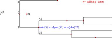
Figure 1: Continuous time Galton–Watson tree.

We end Section 2.1 with some estimates on $N_{t}$ and $D_{t}$. To begin with, the following lemma gives an equivalent for $N_{t}$.

Lemma 2.4.

For $t\in\mathbb{R}_{+}$, we have

$$\mathbb{E}[N_{t}] = \mathrm{e}^{r(m-1)t},$$ (12)

$$\mathbb{E}[N_{t}^{2}] = \cases{\displaystyle\mathrm{e}^{r(m-1)t}+\biggl{(}\frac{\varsigma^{2}}{m-1}+m\biggr{)}\bigl{(}\mathrm{e}^{2r(m-1)t}-\mathrm{e}^{r(m-1)t}\bigr{)},&\quad if $m\not=1$,\cr\displaystyle 1+\varsigma^{2}rt,&\quad if $m=1$.}$$ (13)

If $m>1$, there exists a nonnegative random variable $W$ such that $\{W>0\}=\{\forall t>0,N_{t}>0\}$ a.s., $\mathbb{P}(W>0)>0$ and

$$\lim_{t\rightarrow+\infty}\frac{N_{t}}{\mathbb{E}[N_{t}]}=W\qquad\mbox{a.s. and in }L^{2}.$$ (14)

The process $(N_{t},t\geq 0)$ is a continuous time Markov branching process so that the expectation and the variance of $N_{t}$ are well known (see athreyaney , Chapter III, Section 4). Almost sure convergence toward $W$ is stated again in athreyaney (Theorems 1 and 2, Chapter III, Section 7). Finally, since the martingale $(N_{t}\mathrm{e}^{-r(m-1)t},t\geq 0)$ is bounded in $L^{2}$, we obtain the $L^{2}$ convergence (e.g., Theorem 1.42, page 11 of jacodshiryaev ).

We give the asymptotic behavior of $D_{t}$, the number of deaths before $t$.

Lemma 2.5.

If $m>1$, the following convergence holds a.s. and in $L^{2}$:

$$\lim_{t\rightarrow+\infty}\frac{D_{t}}{\mathbb{E}[D_{t}]}=W$$ (15)

with

$$\mathbb{E}[D_{t}]=(m-1)^{-1}\bigl{(}\mathrm{e}^{r(m-1)t}-1\bigr{)}$$ (16)

and $W$ defined by (14).

First remark that $(D_{t},t\geq 0)$ is a counting process with compensator $(\int_{0}^{t}rN_{s}\,ds,t\geq 0)$. We set $\Delta N_{t}=N_{t}-N_{t-}$ so that $dN_{t}=\Delta N_{t}\,dD_{t}$. To prove (15), it is sufficient to prove that $\mathrm{e}^{-r(m-1)t}I_{t}$ goes to $0$ a.s. and in $L^{2}$, where $I_{t}=(m-1)D_{t}-N_{t}$. Since $I=(I_{t},t\geq 0)$ satisfies the following stochastic equation driven by $(D_{t},t\geq 0)$:

$$dI_{t}=(m-1-\Delta N_{t})\,dD_{t},$$ (17)

we get that $I$ is an $L^{2}$ martingale. We deduce that $d\langle I\rangle_{t}=\varsigma^{2}rN_{t}\,dt$ and

$$\mathbb{E}[I^{2}_{t}] = 1+\mathbb{E}[\langle I\rangle_{t}]=1+\varsigma^{2}r\int_{0}^{t}\mathrm{e}^{r(m-1)s}\,ds$$

$$= 1+\frac{\varsigma^{2}}{m-1}\bigl{(}\mathrm{e}^{r(m-1)t}-1\bigr{)},$$

which implies the $L^{2}$ convergence of $\mathrm{e}^{-r(m-1)t}I_{t}$ to $0$. Besides, the process $(\mathrm{e}^{-r(m-1)t}I_{t},t\geq 0)$ is a supermartingale bounded in $L^{2}$ and hence, the convergence also holds almost surely.

Example 1 ((Yule tree)).

The so-called Yule tree is a continuous time Galton–Watson tree with a deterministic offspring distribution: each individual of the population gives birth to 2 individuals, that is, $p_{2}=1$ (i.e., $p=\delta_{2}$, the Dirac mass at 2). The Yule tree is thus a binary tree whose edges have independent exponential lengths with mean $1/r$. In that case, $W$ is exponential with mean 1 (see, e.g., athreyaney , page 112). We deduce from Lemma 2.4 that, for $t\in\mathbb{R}_{+}$,

$$\mathbb{E}[N_{t}]=\mathrm{e}^{rt}\quad\mbox{and}\quad\mathbb{E}[N_{t}^{2}]=2\mathrm{e}^{2rt}-\mathrm{e}^{rt}.$$ (19)

Notice that (19) is also a consequence of the well-known fact that $N_{t}$ is geometric with parameter $\mathrm{e}^{-rt}$ (see, e.g., harris , page 105).

2.2 Markov process indexed by the continuous time Galton–Watson tree

In this section, we define the Markov process $X_{\mathbb{T}}=(X^{u}_{t},(u,t)\in\mathbb{T})$ indexed by the continuous time Galton–Watson tree $\mathbb{T}$ and with initial condition $\mu$. Branching Markov processes have already been the object of abundant literature (e.g., asmussenhering , asmussenheringbook , athreyaney , ethierkurtz , dawson ). The process that we consider jumps at branching times (nonlocal branching property) but these jumps may be dependent.

Let $(E,{\mathcal{E}})$ be a Polish space. We denote by $\mathcal{P}(E)$ the set of probability measures on $(E,{\mathcal{E}})$.

Definition 2.6.

Let $X=(X_{t},t\geq 0)$ be a càdlàg $E$-valued strong Markov process. Let $\widetilde{F}=(F^{(k)}_{j},1\leq j\leq k,k\in\mathbb{N}^{*})$ be a family of measurable functions from $E\times[0,1]$ to $E$. The continuous time branching Markov (CBM) process $X_{\mathbb{T}}=(X_{t}^{u},(u,t)\in\mathbb{T})$ with offspring distribution $p$, exponential lifetimes with mean $1/r$, offspring position $\widetilde{F}$, underlying motion $X$ and starting distribution $\mu\in{\mathcal{P}}(E)$, is defined recursively as follows:

$\mathbb{T}$ is a continuous time Galton–Watson tree with offspring distribution $p$ and exponential lifetimes with mean $1/r$.

Conditionally on $\mathbb{T}$, $X^{\varnothing}=(X^{\varnothing}_{t},t\in[0,\beta(\varnothing)))$ is distributed as $(X_{t},t\in[0,\beta(\varnothing)))$ with $X_{0}$ distributed as $\mu$.

Conditionally on $\mathbb{T}$ and $X^{\varnothing}$, the initial positions of the first generation offspring $(X^{u}_{\alpha(u)},1\leq u\leq\nu_{\varnothing})$ are given by $(F^{(\nu_{\varnothing})}_{u}(X^{\varnothing}_{\beta(\varnothing)-},\Theta),1\leq u\leq\nu_{\varnothing})$ where $\Theta$ is a uniform random variable on $[0,1]$.

Conditionally on $X^{\varnothing}$, $\nu_{\varnothing}$, $\beta_{\varnothing}$ and $(X^{u}_{\alpha(u)},1\leq u\leq\nu_{\varnothing})$, the tree-indexed Markov processes $(X^{uv}_{\alpha(u)+t},(v,t)\in\theta_{(u,\alpha(u))}\mathbb{T})$ for $1\leq u\leq\nu_{\varnothing}$ are independent and, respectively, distributed as $X_{\mathbb{T}}$ with starting distribution the Dirac mass at $X^{u}_{\alpha(u)}$.

For $x\in E$, we define $\mathbb{P}_{x}(A)=\mathbb{P}(A|X_{0}^{\varnothing}=x)$ for all $A\in\mathcal{F}$ and denote by $\mathbb{E}_{x}$ the corresponding expectation. For $\mu\in\mathcal{P}(E)$ we set in a classical manner $\mathbb{P}_{\mu}(A)=\int_{E}\mathbb{P}_{x}(A)\mu(dx)$ and write $\mathbb{E}_{\mu}$ for the expectation w.r.t. $\mathbb{P}_{\mu}$.

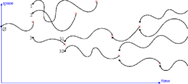
Figure 2: Continuous time Markov process indexed by the Galton–Watson tree of Figure 1.

For $u\in\mathcal{T}$, we extend the definition of $X_{t}^{u}$ when $t\in[0,\alpha(u))$ as follows: $X_{t}^{u}=X_{t}^{u(t)}$, where $u(t)$, defined by (10), is the ancestor of $u$ living at time $t$.

Notice that for $u\in{\mathcal{T}}$, $(X_{t}^{u},t\in[0,\beta(u)))$ does not encode the information about the genealogy of $u$. We remedy this by introducing the following process $(\Lambda^{u}_{t},t\geq 0)$ for $u\in\mathcal{U}$:

$$\Lambda^{u}_{t}=\sum_{v\prec u(t)}\log(\nu_{v}).$$

This process provides the birth times of the ancestors of $u$ as well as their offspring numbers. Notice that it is well defined for all $u\in\mathcal{U}$ contrary to $X_{t}^{u}$. Indeed, the state of $u$ at its birth time, $X_{\alpha(u)}^{u}$, is well defined only for $u\in{\mathcal{T}}$, since it depends on the state of the parent and the number of its offspring.

For $u\in\mathcal{U}$, the process $(\Lambda^{u}_{t},t\in[0,\beta(u)))$ is a compound Poisson process with rate $r$ for the underlying Poisson process $(S^{u}_{t},t\geq 0)$ and increments distributed as $\log(\nu)$ with $\nu$ distributed as $p$, stopped at its $(|u|+1)$th jump.

In the sequel, we denote by $\widetilde{X}^{u}_{t}=(X^{u}_{t},\Lambda^{u}_{t})$ the couple containing the information on the position and genealogy of the particle $u$.

2.3 Measure-valued description

Let $\mathcal{B}_{b}(E,\mathbb{R})$ be the set of real-valued measurable bounded functions on $E$ and ${\mathcal{M}}_{F}(E)$ the set of finite measures on $E$ embedded with the topology of weak convergence. For $\mu\in{\mathcal{M}}_{F}(E)$ and $f\in\mathcal{B}_{b}(E,\mathbb{R})$ we write $\langle\mu,f\rangle=\int_{E}f(x)\mu(dx)$.

We introduce the following measures to represent the population at $t$:

$$\bar{Z}_{t}=\sum_{u\in V_{t}}\delta_{(u,X_{t}^{u})}\quad\mbox{and}\quad{Z}_{t}=\sum_{u\in V_{t}}\delta_{X_{t}^{u}},$$ (20)

where $V_{t}$ has been defined in (8). Note that $\langle Z_{t},f\rangle=\sum_{u\in V_{t}}f(X^{u}_{t})$. Since $X$ is càdlàg, we get that the process $Z=(Z_{t},t\geq 0)$ is a càdlàg measure-valued Markov process of $\mathbb{D}(\mathbb{R}_{+},\mathcal{M}_{F}(E))$.

Following Fournier and Méléard fourniermeleard , we can describe the evolution of $Z$ in terms of stochastic differential equations (SDE). Let $\rho(ds,du,dk,d\theta)$ be a Poisson point measure of intensity $r\,ds\otimes n(du)\otimes p(dk)\otimes d\theta$ where $ds$ and $d\theta$ are Lebesgue measures on $\mathbb{R}_{+}$ and $[0,1]$, respectively, $n(du)$ is the counting measure on $\mathcal{U}$ and $p(dk)=\sum_{i\in\mathbb{N}}p_{i}\delta_{i}(dk)$ is the offspring distribution. This measure $\rho$ gives the information on the branching events. Let $L$ be the infinitesimal generator of $X$. If $\mathcal{C}^{1,0}_{b}(\mathbb{R}_{+}\times E,\mathbb{R})$ denotes the space of continuous bounded functions that are $\mathcal{C}^{1}$ in time with bounded derivatives, then for test functions $f\dvtx(t,x)\mapsto f_{t}(x)$ in $\mathcal{C}^{1,0}_{b}(\mathbb{R}_{+}\times E,\mathbb{R})$ such that $\forall t\in\mathbb{R}_{+},f_{t}\in D(L)$, we have

$$\langle Z_{t},f_{t}\rangle = f_{0}(X^{\varnothing}_{0})+\int_{0}^{t}\int_{\mathbb{R}_{+}}\bigl{(}Lf(x)+\partial_{s}f(x)\bigr{)}Z_{s}(dx)\,ds+W^{f}_{t}$$

$${}+\int_{0}^{t}\int_{\mathcal{U}\times\mathbb{N}\times[0,1]}\mathbf{1}_{\{u\in V_{s-}\}}\Biggl{(}\sum_{j=1}^{k}f_{s}\bigl{(}F^{(k)}_{j}(X^{u}_{s_{-}},\theta)\bigr{)}-f_{s}(X^{u}_{s_{-}})\Biggr{)}$$

$$\hphantom{{}+\int_{0}^{t}\int_{\mathcal{U}\times\mathbb{N}\times[0,1]}}{}\times\rho(ds,du,dk,d\theta),$$

where $W^{f}_{t}$ is a martingale. Explicit expressions of this martingale and of the infinitesimal generator of $(Z_{t},t\geq 0)$ can be obtained when the form of the generator $L$ is given.

Example 2 ((Splitted diffusions)).

The case when the Markov process $X$ is a real diffusion ($E=\mathbb{R}$) is an interesting example. Let $L$ be given by

$$Lf(x)=b(x)f^{\prime}(x)+\frac{\sigma^{2}(x)}{2}f^{\prime\prime}(x),$$ (22)

where we assume that $b$ and $\sigma$ are bounded and Lipschitz continuous. In this case, we can consider the following class of cylindrical functions from $\mathcal{M}_{F}(\mathbb{R})$ into $\mathbb{R}$ defined by $\phi_{f}(Z)=\phi(\langle Z,f\rangle)$ for $f\in\mathcal{C}^{2}_{b}(\mathbb{R},\mathbb{R})$ and $\phi\in\mathcal{C}^{2}_{b}(\mathbb{R})$ which is known to be convergence determining on $\mathcal{P}(\mathcal{M}_{F}(\mathbb{R}))$ (see, e.g., dawson , Theorem 3.2.6). We can define the infinitesimal generator $\mathcal{L}$ of $(Z_{t})_{t\geq 0}$ for these functions as

$$\mathcal{L}\phi_{f}(Z)=\mathcal{L}_{1}\phi_{f}(Z)+\mathcal{L}_{2}\phi_{f}(Z),$$ (23)

where $\mathcal{L}_{1}$ and $\mathcal{L}_{2}$ correspond to the branching and motion parts. Such decompositions were already used in Dawson dawson (Section 2.10) and in Roelly and Rouault roellyrouault , for instance. The generator $\mathcal{L}_{1}$ is defined by

$$\mathcal{L}_{1}\phi_{f}(Z) = r\int_{E}\int_{0}^{1}\sum_{k\in\mathbb{N}}\Biggl{(}\phi\Biggl{(}\langle Z,f\rangle+\sum_{j=1}^{k}f\bigl{(}F^{(k)}_{j}(x,\theta)\bigr{)}-f(x)\Biggr{)}-\phi_{f}(Z)\Biggr{)}$$

$$\hphantom{r\int_{E}\int_{0}^{1}\sum_{k\in\mathbb{N}}}{}\times p_{k}\,d\theta\,Z(dx)$$

with the convention that the sum over $j$ is zero when $k=0$. The generator $\mathcal{L}_{2}$ is given by

$$\mathcal{L}_{2}\phi_{f}(Z)=\langle Z,Lf\rangle\phi^{\prime}(\langle Z,f\rangle)+\langle Z,\sigma(x)f^{\prime 2}(x)\rangle\phi^{\prime\prime}(\langle Z,f\rangle).$$

For a test function $f\dvtx(t,x)\mapsto f_{t}(x)$ in $\mathcal{C}^{1,2}_{b}(\mathbb{R}_{+}\times\mathbb{R},\mathbb{R})$, the evolution of $(Z_{t}$, $t\geq 0)$ can then be described by the following SDE:

$$\langle Z_{t},f_{t}\rangle = f_{0}(X^{\varnothing}_{0})+\int_{0}^{t}\int_{\mathcal{U}\times\mathbb{N}\times[0,1]}\mathbf{1}_{\{u\in V_{s-}\}}\Biggl{(}\sum_{j=1}^{k}f_{s}\bigl{(}F^{(k)}_{j}(X^{u}_{s_{-}},\theta)\bigr{)}-f_{s}(X^{u}_{s_{-}})\Biggr{)}$$

$$\hphantom{f_{0}(X^{\varnothing}_{0})+\int_{0}^{t}\int_{\mathcal{U}\times\mathbb{N}\times[0,1]}}{}\times\rho(ds,du,dk,d\theta)$$

$${}+\int_{0}^{t}\int_{\mathbb{R}}\bigl{(}Lf_{s}(x)+\partial_{s}f_{s}(x)\bigr{)}Z_{s}(dx)\,ds$$

$${}+\int_{0}^{t}\sum_{u\in V_{s}}\sqrt{2}\sigma(X^{u}_{s})\partial_{x}f_{s}(X^{u}_{s})\,dB_{s}^{u},$$

where $(B^{u})_{u\in\mathcal{U}}$ is a family of independent standard Brownian motions. In bansayetran , such splitted diffusions are considered to describe a multi-level population. The cells, which correspond to the individuals in the present setting, undergo binary divisions and contain a continuum of parasites that evolves as a Feller diffusion with drift $b(x)=(b-d)x$ and diffusion $\sigma^{2}(x)=2\sigma^{2}x$. At the branching time $s$ for the individual $u$, each daughter inherits a random fraction of the value of the mother. The daughters $u1$ and $u2$ start, respectively, at $F^{(2)}_{1}(X_{s_{-}}^{u},\theta)=G^{-1}(\theta)X_{s_{-}}^{u}$ and $F^{(2)}_{2}(X_{s_{-}}^{u},\theta)=(1-G^{-1}(\theta))X_{s_{-}}^{u}$, where $G^{-1}$ is the generalized inverse of $G$, the cumulative distribution function of the random fraction.

3 The auxiliary Markov process and Many-to-One formulas

In this section, we are interested in the distribution of the path of an individual picked at random in the population at time $t$. By choosing uniformly among the individuals present at time $t$, we give a more important weight to branches where there have been more divisions and more children since the proportion of the corresponding offspring will be higher. Our pathwise approach generalizes delmasmarsalle (discrete time) and bansayetran (continuous time Yule process). As mentioned in the Introduction, this size bias has already been observed by samuels , bigginsaap76 for the tree structure when considering marginal distributions and by chauvinrouaultwakolbinger , hardyharris3 for local branching Markov process.

In Section 3.1, we introduce an auxiliary Markov process which approximates the distribution of an individual picked at random among all the individuals living at time $t$. The relation between $X_{\mathbb{T}}$ and the auxiliary process also appears when summing the contributions of all individuals of $\mathbb{T}$ (Section 3.2) and of all pairs of individuals (Section 3.3).

3.1 Auxiliary process and Many-to-One formula at fixed time

We focus on the law of an individual picked at random and show that it is obtained from an auxiliary Markov process. This auxiliary Markov process $\widetilde{Y}=(Y,\Lambda)$ has two components. The component $Y$ describes the motion on the space $E$. The second component $\Lambda$ encodes a virtual genealogy and $Y$ can then be seen as the motion along a random lineage of this genealogy. More precisely, $\Lambda$ is a compound Poisson process with rate $rm$; its jump times provide the branching events of the chosen lineage and its jump sizes are related to the offspring number $H$ whose distribution is the size biased distribution of $p$. As for the motion, $Y$ behaves like $X$ between two jumps of $\Lambda$. At these jump times, $Y$ starts from a new position given by $F_{J}^{(H)}(\cdot,\Theta)$ where $J$ is uniform on $\{1,\ldots,H\}$ and $\Theta$ is uniform on $[0,1]$.

For the definition of $\Lambda$, we shall consider the logarithm of the offspring number as this is the quantity that is involved in the Girsanov formulas. Notice that we cannot recover all the jump times from $\Lambda$ unless there is no offspring number equal to 1, that is, $p_{1}=0$. This can, however, always be achieved by changing the value of the jump rate $r$ and adding the jumps related to $F_{1}^{(1)}$ to the process $X$. Henceforth, we assume without loss of generality the following.

Assumption 3.1.

The offspring distribution satisfies $p_{1}=0$.

By convention for a function $f$ defined on an interval $I$, we set $f_{\zeta}=(f(t),t\in\zeta)$ for any $\zeta\subset I$.

Definition 3.2.

Let $X_{\mathbb{T}}$ be as in Definition 2.6 with starting distribution $\mu\in{\mathcal{P}}(E)$. The corresponding auxiliary process $\widetilde{Y}=(Y,\Lambda)$, with $Y=(Y_{t},t\geq 0)$ and $\Lambda=(\Lambda_{t},t\geq 0)$, is an $E\times\mathbb{R}$-valued càdlàg Markov process. The process $(Y,\Lambda)$ and ${\mathcal{I}}=(I_{k},k\in\mathbb{N}^{*})$, a sequence of random variables, are defined as follows:

$\Lambda$ is a compound Poisson process: $\Lambda_{t}=\sum_{k=1}^{S_{t}}\log(H_{k})$, where $S=(S_{t},t\geq 0)$ is a Poisson process with intensity $rm$ and $(H_{k},k\in\mathbb{N}^{*})$ are independent random variables independent of $S$ and with common distribution the size biased distribution of $p$ $(hp_{h}/m,h\in\mathbb{N}^{*})$.

Conditionally on $\Lambda$, $(I_{k},k\in\mathbb{N}^{*})$ are independent random variables and $I_{k}$ is uniform on $\{1,\ldots,H_{k}\}$.

Conditionally on $(\Lambda,{\mathcal{I}})$, $\tau_{1}=\inf\{t\geq 0;S_{t}\neq S_{0}\}$ is known and the process $Y_{[0,\tau_{1})}$ is distributed as $X_{[0,\tau_{1})}$.

Conditionally on $(\Lambda,{\mathcal{I}},Y_{[0,\tau_{1})})$, $Y_{\tau_{1}}$ is distributed as $F^{(H_{1})}_{I_{1}}(Y_{\tau_{1}-},\Theta)$, where $\Theta$ is an independent uniform random variable on $[0,1]$.

The distribution of $(Y_{\tau_{1}+t},t\geq 0)$ conditionally on $(\Lambda,{\mathcal{I}},Y_{[0,\tau_{1}]})$ is equal to the distribution of $Y$ conditionally on $(\Lambda_{\tau_{1}+t}-\Lambda_{\tau_{1}},t\geq 0)$ and $(I_{1+k},k\in\mathbb{N}^{*})$ and started at $Y_{\tau_{1}}$.

We write $\mathbb{E}_{\mu}$ when we take the expectation with respect to $(Y,\Lambda,{\mathcal{I}})$ and the starting measure is $\mu$ for the $Y$ component. We also use the same convention as those described just after Definition 2.6.

The formula (25) in the next proposition is similar to the so-called Many-to-One theorem of Hardy and Harris hardyharris3 (Section 8.2) that enables expectation of sums over particles in the branching process to be calculated in terms of an expectation of an auxiliary process. Notice that in our setting an individual may have no offspring with positive probability (if $p_{0}>0$) which is not the case in hardyharris3 .

Proposition 3.3 ((Many-to-One formula at fixed time)).

For $t\geq 0$ and for any nonnegative measurable function $f\in\mathcal{B}(\mathbb{D}([0,t],E\times\mathbb{R}),\mathbb{R}_{+})$,

$$\frac{\mathbb{E}_{\mu}[\sum_{u\in V_{t}}f(\widetilde{X}^{u}_{[0,t]})]}{\mathbb{E}[N_{t}]}=\mathbb{E}_{\mu}\bigl{[}f\bigl{(}\widetilde{Y}_{[0,t]}\bigr{)}\bigr{]}.$$ (25)

Remark 3.4.

[(1)]

Asymptotically, $N_{t}$ and $\mathbb{E}[N_{t}]$ are of same order on $\{W>0\}$ [see (14)]. Thus, the left-hand side of (25) can be seen as an approximation, for large $t$, of the law of an individual picked at random in $V_{t}$.

For $m>1$, a typical individual living at time $t$ has prolific ancestors with shorter lives. For $m<1$, a typical individual living at time $t$ has still prolific ancestors but with longer lives.

If births are local [i.e., for all $j\leq k$, $F^{(k)}_{j}(x,\theta)=x$], then $Y$ is distributed as $X$.

Proof of Proposition 3.3 Let $\Lambda$ be a compound Poisson process as in Definition 3.2(i). Let us show the following Girsanov formula, for any nonnegative measurable function $g$:

$$\mathbb{E}\bigl{[}g\bigl{(}\Lambda_{[0,t]}\bigr{)}\bigr{]}=\mathbb{E}\bigl{[}g\bigl{(}\Lambda^{\prime}_{[0,t]}\bigr{)}\mathrm{e}^{-r(m-1)t+\Lambda^{\prime}_{t}}\bigr{]},$$ (26)

where the process $\Lambda^{\prime}$ is a compound process with rate $r$ for the underlying Poisson process and increments distributed as $\log(\nu)$ with $\nu$ distributed as $p$. Indeed, $g(\Lambda_{[0,t]})$ is a function of $t$, of the times $\tau_{q}=\inf\{t\geq 0;S_{t}=q\}-\inf\{t\geq 0;S_{t}=q-1\}$ and of jump sizes $\log(H_{q})$ of $\Lambda$,

$$g\bigl{(}\Lambda_{[0,t]}\bigr{)}=\sum_{q=0}^{+\infty}G_{q}(t,\tau_{1},\ldots,\tau_{q},H_{1},\ldots,H_{q})\mathbf{1}_{\{\sum_{i=1}^{q}\tau_{i}\leq t<\sum_{i=1}^{q+1}\tau_{i}\}}$$

for some functions $(G_{q},q\in\mathbb{N})$. We deduce that

$$\mathbb{E}\bigl{[}g\bigl{(}\Lambda_{[0,t]}\bigr{)}\bigr{]}$$

$$\qquad=\sum_{q=0}^{+\infty}\int_{\mathbb{R}_{+}^{q}}\Biggl{(}\sum_{h_{1},\ldots,h_{q}}(rm)^{q}\mathrm{e}^{-rmt}G_{q}(t,t_{1},\ldots,t_{q},h_{1},\ldots,h_{q})$$

$$\hskip 146.0pt\qquad\quad{}\times\prod_{i=1}^{q}\frac{p_{h_{i}}h_{i}}{m}\mathbf{1}_{\{\sum_{i=1}^{q}t_{i}\leq t\}}\Biggr{)}\,dt_{1}\cdots dt_{q}$$

$$\qquad=\sum_{q=0}^{+\infty}\int_{\mathbb{R}_{+}^{q}}\Biggl{(}\sum_{h_{1},\ldots,h_{q}}r^{q}\mathrm{e}^{-rt}G_{q}(t,t_{1},\ldots,t_{q},h_{1},\ldots,h_{q})$$

$$\hphantom{\sum_{q=0}^{+\infty}\int_{\mathbb{R}_{+}^{q}}\Biggl{(}\sum_{h_{1},\ldots,h_{q}}}\qquad\quad{}\times\mathrm{e}^{-r(m-1)t+\sum_{i=1}^{q}\log(h_{i})}\prod_{i=1}^{q}p_{h_{i}}\mathbf{1}_{\{\sum_{i=1}^{q}t_{i}\leq t\}}\Biggr{)}\,dt_{1}\cdots dt_{q}$$

$$\qquad=\mathbb{E}\bigl{[}g\bigl{(}\Lambda^{\prime}_{[0,t]}\bigr{)}\mathrm{e}^{-r(m-1)t+\Lambda^{\prime}_{t}}\bigr{]}.$$

Recall that $(S_{t},t\geq 0)$ [resp., $(S^{u}_{t},t\geq 0)$] is the underlying Poisson process of $\Lambda$ (resp., $\Lambda^{u}$). Notice that if $|u|=q$, then $\{S^{u}_{t}=q\}=\{\alpha(u)\leq t<\beta(u)\}$. We thus deduce from (26) that for $q\in\mathbb{N}$, $u\in{\mathcal{U}}$ such that $|u|=q$,

$$\mathbb{E}\bigl{[}g\bigl{(}\Lambda_{[0,t]}\bigr{)}\mathbf{1}_{\{S_{t}=q\}}\bigr{]}=\mathbb{E}\bigl{[}g\bigl{(}\Lambda^{u}_{[0,t]}\bigr{)}\mathrm{e}^{-r(m-1)t+\Lambda^{u}_{t}}\mathbf{1}_{\{\alpha(u)\leq t<\beta(u)\}}\bigr{]}.$$ (27)

Let $q\in\mathbb{N}^{*}$. By construction, conditionally on $\{\Lambda_{[0,t]}=\lambda_{[0,t]}\}$, $\{S_{t}=q\}$, $\{(I_{1},\ldots,I_{q})=u\}$, $Y_{[0,t]}$ is distributed as $X^{u}_{[0,t]}$ conditionally on $\{\Lambda^{u}_{[0,t]}=\lambda_{[0,t]}\}$. This holds also for $q=0$ with the convention that $(I_{1},\ldots,I_{q})=\varnothing$. Therefore, we have for any nonnegative measurable functions $g$ and $f$,

$$\mathbb{E}_{\mu}\bigl{[}g\bigl{(}\Lambda_{[0,t]}\bigr{)}f\bigl{(}Y_{[0,t]}\bigr{)}\bigr{]}$$

$$\qquad=\sum_{u\in{\mathcal{U}}}\sum_{q\in\mathbb{N}}\mathbf{1}_{\{|u|=q\}}\mathbb{E}_{\mu}\bigl{[}g\bigl{(}\Lambda_{[0,t]}\bigr{)}f\bigl{(}Y_{[0,t]}\bigr{)}\mathbf{1}_{\{(I_{1},\ldots,I_{q})=u\}}\mathbf{1}_{\{S_{t}=q\}}\bigr{]}$$

$$\qquad=\sum_{u\in{\mathcal{U}}}\sum_{q\in\mathbb{N}}\mathbf{1}_{\{|u|=q\}}\mathbb{E}_{\mu}\bigl{[}g\bigl{(}\Lambda_{[0,t]}\bigr{)}\mathbb{E}_{\mu}\bigl{[}f\bigl{(}X^{u}_{[0,t]}\bigr{)}|\Lambda^{u}_{[0,t]}\bigr{]}_{|\Lambda^{u}_{[0,t]}=\Lambda_{[0,t]}}$$

$$\hskip 162.0pt\qquad\quad{}\times\mathbf{1}_{\{(I_{1},\ldots,I_{q})=u\}}\mathbf{1}_{\{S_{t}=q\}}\bigr{]}.$$

Using the points (i) and (ii) of Definition 3.2, we see that

$$\mathbb{P}(I_{1}=u_{1},\ldots,I_{q}=u_{q}|\Lambda_{t},\{S_{t}=q\})$$

$$\qquad=\prod_{k=1}^{q}1/H_{k}=\mathrm{e}^{-\Lambda_{t}}\qquad\mbox{if }u_{1}\leq H_{1},\ldots,u_{q}\leq H_{q}$$

$$\qquad=0\qquad\mbox{otherwise}.$$

Hence,

$$\mathbb{E}_{\mu}\bigl{[}g\bigl{(}\Lambda_{[0,t]}\bigr{)}f\bigl{(}Y_{[0,t]}\bigr{)}\bigr{]}$$

$$\qquad=\sum_{u\in{\mathcal{U}}}\sum_{q\in\mathbb{N}}\mathbf{1}_{\{|u|=q\}}\mathbb{E}_{\mu}\bigl{[}g\bigl{(}\Lambda_{[0,t]}\bigr{)}\mathbb{E}_{\mu}\bigl{[}f\bigl{(}X^{u}_{[0,t]}\bigr{)}|\Lambda^{u}_{[0,t]}\bigr{]}_{|\Lambda^{u}_{[0,t]}=\Lambda_{[0,t]}}$$

$$\hskip 121.6pt\qquad\quad{}\times\mathrm{e}^{-\Lambda_{t}}\mathbf{1}_{\{u_{1}\leq H_{1},\ldots,u_{q}\leq H_{q}\}}\mathbf{1}_{\{S_{t}=q\}}\bigr{]}$$

$$\qquad=\sum_{u\in{\mathcal{U}}}\sum_{q\in\mathbb{N}}\mathbf{1}_{\{|u|=q\}}\mathbb{E}_{\mu}\bigl{[}g\bigl{(}\Lambda^{u}_{[0,t]}\bigr{)}\mathbb{E}_{\mu}\bigl{[}f\bigl{(}X^{u}_{[0,t]}\bigr{)}|\Lambda^{u}_{[0,t]}\bigr{]}\mathrm{e}^{-r(m-1)t}$$

$$\hskip 102.8pt\qquad\quad{}\times\mathbf{1}_{\{u_{1}\leq\nu_{\varnothing},\ldots,u_{q}\leq\nu_{(u_{1},\ldots,u_{q-1})}\}}\mathbf{1}_{\{S^{u}_{t}=q\}}\bigr{]},$$

thanks to (27). Remark that for $u=(u_{1},\ldots,u_{q})$,

$$\bigl{\{}u_{1}\leq\nu_{\varnothing},\ldots,u_{q}\leq\nu_{(u_{1},\ldots,u_{q-1})}\bigr{\}}=\{u\in\mathcal{T}\},$$

and for such $u$, we have $\{S^{u}_{t}=q\}=\{u\in V_{t}\}$ as noticed before. As a consequence,

$$\mathbb{E}_{\mu}\bigl{[}g\bigl{(}\Lambda_{[0,t]}\bigr{)}f\bigl{(}Y_{[0,t]}\bigr{)}\bigr{]}=\sum_{u\in{\mathcal{U}}}\mathbb{E}_{\mu}\bigl{[}g\bigl{(}\Lambda^{u}_{[0,t]}\bigr{)}f\bigl{(}X^{u}_{[0,t]}\bigr{)}\mathrm{e}^{-r(m-1)t}\mathbf{1}_{\{u\in V_{t}\}}\bigr{]}.$$

Finally, we use a monotone class argument to conclude.

3.2 Many-to-One formulas over the whole tree

In this section we generalize identity (25) on the link between the tree indexed process $X_{\mathbb{T}}$ and the auxiliary Markov process $Y$ by considering sums over the whole tree.

Let us consider the space $\mathcal{D}$ of nonnegative measurable functions $f\in\mathcal{B}(\mathbb{R}_{+}\times\mathbb{D}(\mathbb{R}_{+},E\times\mathbb{R}),\mathbb{R}_{+})$ such that $f(t,y)=f(t,z)$ as soon as $y_{[0,t)}=z_{[0,t)}$. By convention, if $y$ is defined at least on $[0,t)$, we will write $f(t,y_{[0,t)})$ for $f(t,z)$ where $z$ is any function such that $z_{[0,t)}=y_{[0,t)}$.

Proposition 3.5 ((Many-to-One formula over the whole tree)).

For all nonnegative measurable function $f$ of $\mathcal{D}$, we have

$$\mathbb{E}_{\mu}\biggl{[}\sum_{u\in{\mathcal{T}}}f\bigl{(}\beta(u),\widetilde{X}^{u}_{[0,\beta(u))}\bigr{)}\biggr{]}=r\int_{0}^{+\infty}ds\,\mathrm{e}^{r(m-1)s}\mathbb{E}_{\mu}\bigl{[}f\bigl{(}s,\widetilde{Y}_{[0,s)}\bigr{)}\bigr{]}.\vspace*{-3pt}$$ (28)

Before coming to the proof of Proposition 3.5, we introduce a notation that will be very useful in the sequel. By convention for two functions $f,g$ defined, respectively, on two intervals $I_{f},I_{g}$, for $[a,b)\subset I_{f}$ and $[c,d)\subset I_{g}$, we define the concatenation $[f_{[a,b)};g_{[c,d)}]=h_{J}$ where $J=[a,b+(d-c))$,

$$h(t)=\cases{f(t),&\quad if $t\in[a,b)$,\cr g\bigl{(}c+(t-b)\bigr{)},&\quad if $t\in[b,d-c+b)$.}\vspace*{-3pt}$$

Proof of Proposition 3.5 We first notice that if $\tau$ is an exponential random variable with mean $1/r$ ($r>0$), then we have, for any nonnegative measurable function $g$,

$$\mathbb{E}\biggl{[}r\int_{0}^{\tau}g(t)\,dt\biggr{]}=\mathbb{E}[g(\tau)].$$ (29)

Besides, we have

$$\mathbb{E}_{\mu}\bigl{[}\mathbf{1}_{\{u\in\mathcal{T}\}}f\bigl{(}\beta(u),\widetilde{X}^{u}_{[0,\beta(u))}\bigr{)}\bigr{]}=\mathbb{E}_{\mu}\bigl{[}\mathbf{1}_{\{u\in\mathcal{T}\}}f\bigl{(}\beta(u),\bigl{[}\widetilde{X}^{u}_{[0,\alpha(u))};\widetilde{X}_{[0,\beta(u)-\alpha(u))}\bigr{]}\bigr{)}\bigr{]},$$

where conditionally on $\widetilde{X}^{u}_{[0,\alpha(u))}$, $\beta(u)$, $\{u\in\mathcal{T}\}$, $\widetilde{X}=(X,c)$ with $X$ of distribution $\mathbb{P}_{X^{u}_{\alpha(u)}}$ and $c$ the constant process equal to $\Lambda^{u}_{\alpha(u)}$. Notice that we have chosen $\widetilde{X}$ independent of $\beta(u)$. Thus, conditioning with respect to $[\widetilde{X}^{u}_{[0,\alpha(u))};\widetilde{X}_{[0,+\infty)}]$, $\{u\in{\mathcal{T}}\}$ and using (29), we get

$$\mathbb{E}_{\mu}\bigl{[}\mathbf{1}_{\{u\in\mathcal{T}\}}f\bigl{(}\beta(u),\widetilde{X}^{u}_{[0,\beta(u))}\bigr{)}\bigr{]}$$

$$\qquad=r\mathbb{E}\biggl{[}\mathbf{1}_{\{u\in\mathcal{T}\}}\int_{0}^{\beta(u)-\alpha(u)}\,ds\,f\bigl{(}\alpha(u)+s,\widetilde{X}^{u}_{[0,\alpha(u)+s)}\bigr{)}\biggr{]}.$$

We deduce,

$$\mathbb{E}_{\mu}\bigl{[}\mathbf{1}_{\{u\in\mathcal{T}\}}f\bigl{(}\beta(u),\widetilde{X}^{u}_{[0,\beta(u))}\bigr{)}\bigr{]} = r\mathbb{E}\biggl{[}\mathbf{1}_{\{u\in\mathcal{T}\}}\int_{\alpha(u)}^{\beta(u)}ds\,f\bigl{(}s,\widetilde{X}^{u}_{[0,s)}\bigr{)}\biggr{]}$$

$$= r\int_{0}^{+\infty}ds\,\mathbb{E}\bigl{[}\mathbf{1}_{\{u\in V_{s}\}}f\bigl{(}s,\widetilde{X}^{u}_{[0,s)}\bigr{)}\bigr{]}.$$

Using Proposition 3.3, we get

$$\mathbb{E}_{\mu}\biggl{[}\sum_{u\in{\mathcal{T}}}f\bigl{(}\beta(u),\widetilde{X}^{u}_{[0,\beta(u))}\bigr{)}\biggr{]} = r\int_{0}^{+\infty}ds\,\mathbb{E}_{\mu}\biggl{[}\sum_{u\in V_{s}}f\bigl{(}s,\widetilde{X}^{u}_{[0,s)}\bigr{)}\biggr{]}$$

$$= r\int_{0}^{+\infty}ds\,\mathrm{e}^{r(m-1)s}\mathbb{E}_{\mu}\bigl{[}f\bigl{(}s,\widetilde{Y}_{[0,s)}\bigr{)}\bigr{]}.$$

The equality (28) means that adding the contributions over all the individuals in the Galton–Watson tree corresponds (at least for the first moment) to integrating the contribution of the auxiliary process over time with an exponential weight $\mathrm{e}^{r(m-1)t}$ which is the average number of living individuals at time $t$. Notice the weight is increasing if the Galton–Watson tree is supercritical and decreasing if it is subcritical.

Remark 3.6.

We shall give two alternative formulas for (28). [(1)]

We deduce from (28) that, for all nonnegative measurable function $f$,

$$\mathbb{E}_{\mu}\biggl{[}\sum_{u\in{\mathcal{T}}}f\bigl{(}\beta(u),\widetilde{X}^{u}_{[0,\beta(u))}\bigr{)}\biggr{]}=\mathbb{E}_{\mu}\bigl{[}f\bigl{(}\tau,\widetilde{Y}_{[0,\tau)}\bigr{)}\mathrm{e}^{rm\tau}\bigr{]},$$ (30)

where $\tau$ is an independent exponential random variable of mean $1/r$. Thus, the right-hand side of equation (28) can be read as the expectation of a functional of the process $\widetilde{Y}$ up to an independent exponential time $\tau$ of mean $1/r$ with a weight $\mathrm{e}^{rm\tau}$.

Let $\tau_{q}=\inf\{t\geq 0;S_{t}=q\}$ the time of the $q$th jump for the compound Poisson process $\Lambda$. Using (29), it is easy to check that, for any nonnegative measurable function $g$,

$$\frac{1}{m}\sum_{q\geq 1}\mathbb{E}_{\mu}\bigl{[}g\bigl{(}\widetilde{Y}_{[0,\tau_{q})},\tau_{q}\bigr{)}\bigr{]}=r\int_{0}^{+\infty}\mathbb{E}_{\mu}\bigl{[}g\bigl{(}\widetilde{Y}_{[0,s)},s\bigr{)}\bigr{]}\,ds.$$

Therefore, we deduce from (28) that, for all nonnegative measurable function $f$,

$$\mathbb{E}_{\mu}\biggl{[}\sum_{u\in{\mathcal{T}}}f\bigl{(}\beta(u),\widetilde{X}^{u}_{[0,\beta(u))}\bigr{)}\biggr{]}=\frac{1}{m}\sum_{q\geq 1}\mathbb{E}_{\mu}\bigl{[}f\bigl{(}\tau_{q},\widetilde{Y}_{[0,\tau_{q})}\bigr{)}\mathrm{e}^{r(m-1)\tau_{q}}\bigr{]}.$$ (31)

This formula emphasizes that the jumps of the auxiliary process correspond to death times in the tree.

3.3 Identities for forks

In order to compute second moments, we shall need the distribution of two individuals picked at random in the whole population and which are not in the same lineage. As in the Many-to-One formula, it will involve the auxiliary process.

First, we define the following sets of forks:

$$\quad\mathcal{FU}=\{(u,v)\in\mathcal{U}^{2}\dvtx|u\wedge v|<\min(|u|,|v|)\}\quad\mbox{and}\quad\mathcal{FT}=\mathcal{FU}\cap\mathcal{T}^{2}.$$ (32)

Let $\widetilde{J}_{2}$ be the operator defined for all nonnegative measurable function $f$ from $(E\times\mathbb{R})^{2}$ to $\mathbb{R}$ by

$$\widetilde{J}_{2}f(x,\lambda) = \int_{0}^{1}\mathop{\sum_{(a,b)\in(\mathbb{N}^{*})^{2}}}_{a\neq b}\sum_{k\geq\max(a,b)}p_{k}f\bigl{(}F^{(k)}_{a}(x,\theta),\lambda+\log(k),$$

$$\hphantom{\int_{0}^{1}\mathop{\sum_{(a,b)\in(\mathbb{N}^{*})^{2}}}_{a\neq b}\sum_{k\geq\max(a,b)}p_{k}f\bigl{(}}\hskip 3.0ptF^{(k)}_{b}(x,\theta),\lambda+\log(k)\bigr{)}\,d\theta.$$

Informally, the functional $\widetilde{J}_{2}$ describes the starting positions of two siblings. Notice that we have

$$\widetilde{J}_{2}f(x,\lambda) = m\int_{0}^{1}\mathbb{E}\bigl{[}(H-1)f\bigl{(}F^{(H)}_{I}(x,\theta),\lambda+\log(H),$$

$$\hphantom{m\int_{0}^{1}\mathbb{E}\bigl{[}(H-1)f\bigl{(}}\hskip 2.6ptF^{(H)}_{K}(x,\theta),\lambda+\log(H)\bigr{)}\bigr{]}\,d\theta,$$

where $H$ has the size-biased offspring distribution and conditionally on $H$, $(I,K)$ is distributed as a drawing of a couple without replacement among the integers $\{1,\ldots,H\}$.

For measurable real functions $f$ and $g$ on $E\times\mathbb{R}$, we denote by $f\otimes g$ the real measurable function on $(E\times\mathbb{R})^{2}$ defined by: $(f\otimes g)(\widetilde{x},\widetilde{y})=f(\widetilde{x})g(\widetilde{y})$ for $\widetilde{x},\widetilde{y}\in E\times\mathbb{R}$.

Proposition 3.7 ((Many-to-One formula for forks over the whole tree)).

For all nonnegative measurable functions $\varphi,\psi\in\mathcal{D}$, we have

$$\mathbb{E}_{\mu}\biggl{[}\sum_{(u,v)\in\mathcal{FT}}\varphi\bigl{(}\beta(u),\widetilde{X}^{u}_{[0,\beta(u))}\bigr{)}\psi\bigl{(}\beta(v),\widetilde{X}^{v}_{[0,\beta(v))}\bigr{)}\biggr{]}$$

$$\qquad=\mathbb{E}_{\mu}\bigl{[}\mathrm{e}^{rm\tau}\widetilde{J}_{2}\bigl{(}{\mathbb{E}}_{\cdot}^{\prime}\bigl{[}\varphi\bigl{(}t+{\tau^{\prime}},\bigl{[}\widetilde{y}_{[0,t)};\widetilde{Y}^{\prime}_{[0,{\tau^{\prime}})}\bigr{]}\bigr{)}\mathrm{e}^{rm{\tau^{\prime}}}\bigr{]}_{|t=\tau,\widetilde{y}=\widetilde{Y}}$$ (35)

$$\hphantom{\mathbb{E}_{\mu}\bigl{[}\mathrm{e}^{rm\tau}\widetilde{J}_{2}\bigl{(}}\qquad\quad{}\otimes\mathbb{E}_{\cdot}^{\prime}\bigl{[}\psi\bigl{(}t+{\tau^{\prime}},\bigl{[}\widetilde{y}_{[0,t)};\widetilde{Y}^{\prime}_{[0,{\tau^{\prime}})}\bigr{]}\bigr{)}\mathrm{e}^{rm{\tau^{\prime}}}\bigr{]}_{|t=\tau,\widetilde{y}=\widetilde{Y}}\bigr{)}(\widetilde{Y}_{\tau-})\bigr{]},$$

where, under $\mathbb{E}_{\mu}$, $\tau$ is exponential with mean $1/r$ independent of $\widetilde{Y}$ and, under $\mathbb{E}^{\prime}_{x,\lambda}$, $(\widetilde{Y}^{\prime},{\tau^{\prime}})$ is distributed as $((Y,\Lambda+\lambda),\tau)$ under $\mathbb{E}_{x}$.

Notice that $\{(u,v)\in\mathcal{FU}\}$ is equal to $\{\exists(w,\widetilde{u},\widetilde{v})\in\mathcal{U}^{3},\exists(a,b)\in(\mathbb{N}^{*})^{2},a\neq b,u=wa\widetilde{u},v=wb\widetilde{v}\}$. Let $A$ be the left-hand side of (3.7). We have

$$A = \sum_{w\in\mathcal{U}}\mathop{\sum_{a,b\in\mathbb{N}^{*}}}_{a\not=b}\sum_{\widetilde{u},\widetilde{v}\in\mathcal{U}}\mathbb{E}_{\mu}\bigl{[}\varphi\bigl{(}\beta(w)+\bigl{(}\beta(wa\widetilde{u})-\beta(w)\bigr{)},$$

$$\hphantom{\sum_{w\in\mathcal{U}}\mathop{\sum_{a,b\in\mathbb{N}^{*}}}_{a\not=b}\sum_{\widetilde{u},\widetilde{v}\in\mathcal{U}}\mathbb{E}_{\mu}\bigl{[}\varphi\bigl{(}}\hskip 3.4pt\bigl{[}\widetilde{X}^{w}_{[0,\beta(w))};\widetilde{X}^{wa\widetilde{u}}_{[\beta(w),\beta(wa\widetilde{u}))}\bigr{]}\bigr{)}\mathbf{1}_{\{wa\widetilde{u}\in\mathcal{T}\}}$$

$$\hphantom{\sum_{w\in\mathcal{U}}\mathop{\sum_{a,b\in\mathbb{N}^{*}}}_{a\not=b}\sum_{\widetilde{u},\widetilde{v}\in\mathcal{U}}\mathbb{E}_{\mu}\bigl{[}}{}\times\psi\bigl{(}\beta(w)+\bigl{(}\beta(wb\widetilde{v})-\beta(w)\bigr{)},$$

$$\hskip 120.0pt\bigl{[}\widetilde{X}^{w}_{[0,\beta(w))};\widetilde{X}^{wb\widetilde{v}}_{[\beta(w),\beta(wb\widetilde{v}))}\bigr{]}\bigr{)}\mathbf{1}_{\{wb\widetilde{v}\in\mathcal{T}\}}\bigr{]}.$$

Using the strong Markov property at time $\beta(w)$, the conditional independence between descendants and Proposition 3.5, we get

$$A = \sum_{w\in\mathcal{U}}\mathop{\sum_{a,b\in\mathbb{N}^{*}}}_{a\not=b}\mathbb{E}_{\mu}\bigl{[}\mathbb{E}^{\prime}_{\widetilde{X}^{wa}_{\alpha(wa)}}\bigl{[}\varphi\bigl{(}t+{\tau^{\prime}},\bigl{[}\widetilde{x}_{[0,t)};\widetilde{Y}_{[0,{\tau^{\prime}})}\bigr{]}\bigr{)}\mathrm{e}^{rm{\tau^{\prime}}}\bigr{]}_{|t=\beta(w),\widetilde{x}=\widetilde{X}^{w}}\mathbf{1}_{\{wa\in\mathcal{T}\}}$$

$$\hskip 62.01pt{}\times\mathbb{E}^{\prime}_{\widetilde{X}^{wb}_{\alpha(wb)}}\bigl{[}\psi\bigl{(}t+{\tau^{\prime}},\bigl{[}\widetilde{x}_{[0,t)};\widetilde{Y}_{[0,{\tau^{\prime}})}\bigr{]}\bigr{)}\mathrm{e}^{rm{\tau^{\prime}}}\bigr{]}_{|t=\beta(w),\widetilde{x}=\widetilde{X}^{w}}$$

$$\hskip 255.3pt{}\times\mathbf{1}_{\{wb\in\mathcal{T}\}}\bigr{]},$$

where under $\mathbb{E}^{\prime}_{x,\lambda}$, $(\widetilde{Y}^{\prime},{\tau^{\prime}})$ is distributed as $((Y,\Lambda+\lambda),\tau)$ under $\mathbb{E}_{x}$. As $\{wa,wb\in\mathcal{T}\}=\{w\in\mathcal{T}\}\cap\{\max\{a,b\}\leq\nu_{w}\}$ we have

$$\qquad A = \sum_{w\in\mathcal{U}}\mathbb{E}_{\mu}\bigl{[}\mathbf{1}_{\{w\in\mathcal{T}\}}\widetilde{J}_{2}\bigl{(}{\mathbb{E}}_{\cdot}^{\prime}\bigl{[}\varphi\bigl{(}t+{\tau^{\prime}},\bigl{[}\widetilde{x}_{[0,t)};\widetilde{Y}^{\prime}_{[0,{\tau^{\prime}})}\bigr{]}\bigr{)}\mathrm{e}^{rm{\tau^{\prime}}}\bigr{]}_{|t=\beta(w),\widetilde{x}=\widetilde{X}^{w}}$$

$$\hskip 79.5pt{}\otimes{\mathbb{E}}_{\cdot}^{\prime}\bigl{[}\psi\bigl{(}t+{\tau^{\prime}},\bigl{[}\widetilde{x}_{[0,t)};\widetilde{Y}^{\prime}_{[0,{\tau^{\prime}})}\bigr{]}\bigr{)}\mathrm{e}^{rm{\tau^{\prime}}}\bigr{]}_{|t=\beta(w),\widetilde{x}=\widetilde{X}^{w}}\bigr{)}$$

$$\hskip 250.1pt{}\times\bigl{(}\widetilde{X}^{w}_{\beta(w)_{-}}\bigr{)}\bigr{]}$$

with $\widetilde{J}_{2}$ defined by (3.3). The function under the expectation in (3.3) depends on $\beta(w)$ and $\widetilde{X}^{w}_{[0,\beta(w))}$. Equality (30) then gives the result.

We shall give a version of Proposition 3.7 when the functions of the path depend only on the terminal value of the path. We shall define $J_{2}$ as a simpler version of $\widetilde{J}_{2}$ [see definition (3.3)] acting only on the spatial motion; for all nonnegative measurable function $f$ from $E^{2}$ to $\mathbb{R}$,

$$J_{2}f(x)=m\int_{0}^{1}\mathbb{E}\bigl{[}(H-1)f\bigl{(}F^{(H)}_{I}(x,\theta),F^{(H)}_{K}(x,\theta)\bigr{)}\bigr{]}\,d\theta,$$ (38)

where $(H,I,K)$ are as in (3.3).

As a direct consequence of Proposition 3.7 and of the fact that $Y$ is càdlàg, we have the following corollary.

Corollary 3.8 ((Many-to-One formula for forks over the whole tree)).

Let $({Q}_{t},t\geq 0)$ be the transition semi-group of ${Y}$. For all nonnegative measurable functions $f,g\in\mathcal{D}$, we have

$$\mathbb{E}_{\mu}\biggl{[}\sum_{(u,v)\in\mathcal{FT}}f\bigl{(}\beta(u),{X}^{u}_{\beta(u)-}\bigr{)}g\bigl{(}\beta(v),{X}^{v}_{\beta(v)-}\bigr{)}\biggr{]}$$

(39)

$$\qquad=r^{3}\int_{[0,\infty)^{3}}\mathrm{e}^{r(m-1)(s+t+t^{\prime})}\,ds\,dt\,dt^{\prime}\,\mu{Q}_{s}\bigl{(}J_{2}({Q}_{t}f_{t+s}\otimes{Q}_{t^{\prime}}g_{t^{\prime}+s})\bigr{)},$$

where $f_{t}(x)=f(t,x)$ and $g_{t}(x)=g(t,x)$ for $t\geq 0$ and $x\in E$.

We can also derive a Many-to-One formula for forks at fixed time.

Proposition 3.9 ((Many-to-One formula for forks at fixed time)).

Let $t\in\mathbb{R}_{+}$ and $\varphi,\psi$ be two nonnegative measurable functions on $\mathbb{D}([0,t],E)$. Then

$$\mathbb{E}_{\mu}\biggl{[}\mathop{\sum_{(u,v)\in V_{t}^{2}}}_{u\not=v}\varphi\bigl{(}\widetilde{X}^{u}_{[0,t]}\bigr{)}\psi\bigl{(}\widetilde{X}^{v}_{[0,t]}\bigr{)}\biggr{]}$$

$$\qquad=r\mathrm{e}^{2r(m-1)t}\int_{0}^{t}da\bigl{(}\mathrm{e}^{-r(m-1)a}\mathbb{E}_{\mu}\bigl{[}\widetilde{J}_{2}\bigl{(}{\mathbb{E}}_{\cdot}^{\prime}\bigl{[}\varphi\bigl{(}\bigl{[}\widetilde{y}_{[0,a)};\widetilde{Y}^{\prime}_{[0,t-a]}\bigr{]}\bigr{)}\bigr{]}_{|\widetilde{y}=\widetilde{Y}}$$ (40)

$$\qquad\quad\hskip 149.0pt{}\otimes{\mathbb{E}}_{\cdot}^{\prime}\bigl{[}\psi\bigl{(}\bigl{[}\widetilde{y}_{[0,a)};\widetilde{Y}^{\prime}_{[0,t-a]}\bigr{]}\bigr{)}\bigr{]}_{|\widetilde{y}=\widetilde{Y}}\bigr{)}(\widetilde{Y}_{a})\bigr{]}\bigr{)},$$

where, under $\mathbb{E}^{\prime}_{x,\lambda}$, $\widetilde{Y}^{\prime}$ is distributed as $(Y,\Lambda+\lambda)$ under $\mathbb{E}_{x}$.

The left-hand side of (3.9) approximates the distribution of a pair of individuals uniformly chosen from the population at time $t$. Indeed, we have in the right-hand side of (3.9) an exponential weight $\mathrm{e}^{2r(m-1)t}$ and thanks to Lemma 2.4, we know that $\mathbb{E}[N_{t}(N_{t}-1)]\sim C\mathrm{e}^{2r(m-1)t}$. The distribution of the paths associated with a random pair is described by the law of forks constituted of independent portions of the auxiliary process $\widetilde{Y}$ and splitted at a time $a\in[0,t]$. Notice that (3.9) indicates that the fork splits at an exponential random time with mean $1/r(m-1)$, conditioned to be less than $t$.

Proof of Proposition 3.9 The proof is similar to the proof of Proposition 3.7 except that we use Proposition 3.3 instead of Proposition 3.5 to obtain an analogue of (3.3).

4 Law of large numbers

In this section, we are interested in averages over the population living at time $t$ for large $t$. When the Galton–Watson tree is not supercritical we have almost sure extinction and thus, we assume here that $m>1$.

4.1 Results and comments

Notice that $N_{t}=0$ implies $Z_{t}=0$ and by convention we set $Z_{t}/N_{t}=0$ in this case. For $t\in\mathbb{R}_{+}$ and $f$ a real function defined on $E$, we derive laws of large numbers for

$$\frac{\langle Z_{t},f\rangle}{N_{t}}=\frac{\sum_{u\in V_{t}}f(X_{t}^{u})}{N_{t}}\quad\mbox{and}\quad\frac{\langle Z_{t},f\rangle}{\mathbb{E}[N_{t}]}=\frac{\sum_{u\in V_{t}}f(X_{t}^{u})}{\mathbb{E}[N_{t}]},$$ (41)

provided the auxiliary process introduced in the previous section satisfies some ergodic conditions.

Let $(Q_{t},t\geq 0)$ be the semigroup of the auxiliary process $Y$ of Definition 3.2,

$$\mathbb{E}_{\mu}[f(Y_{t})]=\mu Q_{t}f$$ (42)

for all $\mu\in{\mathcal{P}}(E)$ and $f$ nonnegative. Recall the operator $J_{2}$ defined in (38).

We shall consider the following ergodicity and integrability assumptions on $f$, a real measurable function defined on $E$, and on $\mu\in{\mathcal{P}}(E)$. [(H4)]

There exists a nonnegative finite measurable function $g$ such that $Q_{t}|f|(x)\leq g(x)$ for all $t\geq 0$ and $x\in E$.

There exists $\pi\in{\mathcal{P}}(E)$ such that $\langle\pi,|f|\rangle<+\infty$ and for all $x\in E$, $\lim_{t\rightarrow+\infty}Q_{t}f(x)=\langle\pi,f\rangle$.

There exists $\alpha<r(m-1)$ and $c_{1}>0$ such that $\mu Q_{t}f^{2}\leq c_{1}\mathrm{e}^{\alpha t}$ for every $t\geq 0$.

There exists $\alpha<r(m-1)$ and $c_{2}>0$ such that $\mu Q_{t}J_{2}(g\otimes g)\leq c_{2}\mathrm{e}^{\alpha t}$ for every $t\geq 0$ with $g$ defined in (H1). Notice that in (H3) and (H4), the constants $\alpha,c_{1}$ and $c_{2}$ may depend on $f$ and $\mu$.

Remark 4.1.

When the auxiliary process $Y$ is ergodic [i.e., $Y$ converges in distribution to $\pi\in{\mathcal{P}}(E)$], the class of continuous bounded functions satisfies (H1)–(H4) with $g$ constant and $\alpha=0$. In some applications, one may have to consider polynomially growing functions. This is why we shall consider hypotheses (H1)–(H4) instead of the ergodic property in Theorem 4.2 or in Proposition 4.3.

The next theorem states the law of large numbers; the asymptotic empirical measure is distributed as the stationary distribution $\pi$ of $Y$.

Theorem 4.2.

For any $\mu\in\mathcal{P}(E)$ and any real measurable function $f$ defined on $E$ satisfying (H1)–(H4), we have

$$\lim_{t\rightarrow+\infty}\frac{\langle Z_{t},f\rangle}{\mathbb{E}[N_{t}]} = \langle\pi,f\rangle W\qquad\mbox{in $L^{2}(\mathbb{P}_{\mu})$,}$$ (43)

$$\lim_{t\rightarrow+\infty}\frac{\langle Z_{t},f\rangle}{N_{t}} = \langle\pi,f\rangle\mathbf{1}_{\{W\neq 0\}}\qquad\mbox{in $\mathbb{P}_{\mu}$-probability}$$ (44)

with $W$ defined by (14) and $\pi$ defined in (H2).

For the proof which is postponed to Section 4.2, we use ideas developed in delmasmarsalle in a discrete time setting. We give an intuition of the result. According to Proposition 3.3, an individual chosen at random at time $t$ is heuristically distributed as $Y_{t}$, that is, as $\pi$ for large $t$ thanks to the ergodic property of $Y$ [see (H2)]. Moreover, two individuals chosen at random among the living individuals at time $t$ have a MRCA who died early which implies that they behave almost independently. Since Lemma 2.4 implies that the number of individuals alive at time $t$ grows to infinity on $\{W\neq 0\}$, this yields the LLN stated in Theorem 4.2.

Notice that Theorem 1.1 is a direct consequence of Theorem 4.2 and Remark 4.1.

We also present a LLN when summing over the set of all individuals who died before time $t$. Recall that $D_{t}=\sum_{u\in\mathcal{T}}\mathbf{1}_{\{\beta(u)<t\}}$ denotes its cardinal.

Recall $S$ in Definition 3.2. Notice that $\mathbb{E}[S_{t}]=rmt$. We shall consider a slightly stronger hypothesis than (H3): [(H5)]

There exists $\alpha<r(m-1)$ and $c_{3}>0$ such that $\mathbb{E}_{\mu}[f^{2}(Y_{t})S_{t}]\leq c_{3}\mathrm{e}^{\alpha t}$ for every $t\geq 0$.

Proposition 4.3.

For any $\mu\in\mathcal{P}(E)$ and any nonnegative measurable function $f$ defined on $E$ satisfying (H1)–(H5), we have

$$\quad\lim_{t\rightarrow+\infty}\frac{\sum_{u\in\mathcal{T}}f(X^{u}_{\beta(u)-})\mathbf{1}_{\{\beta(u)<t\}}}{\mathbb{E}[D_{t}]} = \langle\pi,f\rangle W\qquad\mbox{in $L^{2}(\mathbb{P}_{\mu})$},$$ (45)

$$\lim_{t\rightarrow+\infty}\mathbf{1}_{\{N_{t}>0\}}\frac{\sum_{u\in\mathcal{T}}f(X^{u}_{\beta(u)-})\mathbf{1}_{\{\beta(u)<t\}}}{D_{t}} = \langle\pi,f\rangle\mathbf{1}_{\{W\neq 0\}}$$ (47)

$$\eqntext{\mbox{in $\mathbb{P}_{\mu}$-probability}}$$

with $W$ defined by (14) and $\pi$ defined in (H2).

We can then extend these results to path dependent functions. In particular, the next theorem describes the asymptotic distribution of the motion and lineage of an individual taken at random in the tree. In order to avoid a set of complicated hypothesis we shall assume that $Y$ is ergodic with limit distribution $\pi$ and consider bounded functions.

Theorem 4.4.

We assume that there exists $\pi\in{\mathcal{P}}(E)$ such that for all $x\in E$, and all real-valued bounded measurable function $f$ defined on $E$, $\lim_{t\rightarrow\infty}Q_{t}f(x)=\langle\pi,f\rangle$. Let $T>0$. For any real bounded measurable function $\varphi$ on $\mathbb{D}([0,T],E\times\mathbb{R}_{+})$, we have

$$\lim_{t\rightarrow\infty}\frac{1}{\mathbb{E}[N_{t}]}\sum_{u\in V_{t}}\varphi\bigl{(}X^{u}_{[t-T,t]},\Lambda^{u}_{[t-T,t]}-\Lambda^{u}_{t-T}\bigr{)}$$

$$\qquad=\mathbb{E}_{\pi}\bigl{[}\varphi\bigl{(}\widetilde{Y}_{[0,T]}\bigr{)}\bigr{]}W\qquad\mbox{in $L^{2}(\mathbb{P}_{\mu})$,}$$

$$\lim_{t\rightarrow\infty}\frac{1}{N_{t}}\sum_{u\in V_{t}}\varphi\bigl{(}X^{u}_{[t-T,t]},\Lambda^{u}_{[t-T,t]}-\Lambda^{u}_{t-T}\bigr{)}$$

$$\qquad=\mathbb{E}_{\pi}\bigl{[}\varphi\bigl{(}\widetilde{Y}_{[0,T]}\bigr{)}\bigr{]}\mathbf{1}_{\{W\neq 0\}}\qquad\mbox{in $\mathbb{P}_{\mu}$-probability}$$

with $W$ defined by (14).

Let ${J}_{1}$ be the following operator associated with the possible jumps of $Y$: for all nonnegative measurable function $f$ from $E$ to $\mathbb{R}$,

$$J_{1}f(x)=m\int_{0}^{1}\mathbb{E}\bigl{[}f\bigl{(}F^{(H)}_{I}(x,\theta)\bigr{)}\bigr{]}\,d\theta,$$ (48)

where $H$ has the size-biased offspring distribution and, conditionally on $H$, $I$ is uniform on $\{1,\ldots,H\}$.

Proposition 4.5.

We assume that there exists $\pi\in{\mathcal{P}}(E)$ such that for all $x\in E$, and all real-valued bounded measurable function $f$ defined on $E$, $\lim_{t\rightarrow\infty}Q_{t}f(x)=\langle\pi,f\rangle$.

Let $\varphi$ be a real bounded measurable function defined on $E$-valued paths. We set for $x\in E$, $f(x)=\mathbb{E}_{x}[\varphi(Y_{[0,\tau_{1})})]$, with $\tau_{1}$ from Definition 3.2. Then,

$$\lim_{t\rightarrow+\infty}\frac{\sum_{u\in\mathcal{T}}\varphi(X^{u}_{[\alpha(u),\beta(u))})\mathbf{1}_{\{\beta(u)<t\}}}{\mathbb{E}[D_{t}]} = \langle\pi,J_{1}f\rangle W\quad\mbox{in $L^{2}(\mathbb{P}_{\mu})$},$$

$$\hskip 25.0pt\lim_{t\rightarrow+\infty}\mathbf{1}_{\{N_{t}>0\}}\frac{\sum_{u\in\mathcal{T}}\varphi(X^{u}_{[\alpha(u),\beta(u))})\mathbf{1}_{\{\beta(u)<t\}}}{D_{t}} = \langle\pi,J_{1}f\rangle\mathbf{1}_{\{W\neq 0\}}$$ (49)

$$\eqntext{\mbox{in $\mathbb{P}_{\mu}$-probability}}\quad$$ (50)

with $W$ defined by (14).

Remark 4.6.

The hypothesis on $Y$ in Theorem 4.4 and Proposition 4.5 is slightly stronger than the ergodic condition (i.e., $Y$ converges in distribution to $\pi$), but it is fulfilled if $Y$ converges to $\pi$ for the distance in total variation [i.e., for all $x\in E$, $\lim_{t\rightarrow\infty}\sup_{A\in{\mathcal{E}}}|\mathbb{P}_{x}(Y_{t}\in A)-\pi(A)|=0$]. This property is very common for ergodic processes.

4.2 Proofs

Proof of Theorem 4.2 We assume (H1)–(H4). We shall first prove (43) for $f$ such that $\langle\pi,f\rangle=0$. We have

$$\mathbb{E}_{\mu}\biggl{[}\frac{\langle Z_{t},f\rangle^{2}}{\mathbb{E}[N_{t}]^{2}}\biggr{]}=A_{t}+B_{t},$$

where

$$A_{t}=\mathbb{E}[N_{t}]^{-2}\mathbb{E}_{\mu}\biggl{[}\sum_{u\in V_{t}}f^{2}(X_{t}^{u})\biggr{]}$$

and

$$B_{t}=\mathbb{E}[N_{t}]^{-2}\mathbb{E}_{\mu}\biggl{[}\mathop{\sum_{(u,v)\in V_{t}^{2}}}_{u\neq v}f(X_{t}^{u})f(X_{t}^{v})\biggr{]}.$$

Notice that

$$A_{t}=\mathrm{e}^{-r(m-1)t}\mathbb{E}_{\mu}[f^{2}(Y_{t})]=\mathrm{e}^{-r(m-1)t}\mu Q_{t}f^{2}\mathop{\longrightarrow}_{t\rightarrow\infty}0$$ (51)

thanks to (12) and (25) for the first equality and (H3) for the convergence. We focus now on $B_{t}$. Proposition 3.9 and then (H1) and (H4) imply that

$$\mathbb{E}[N_{t}]^{-2}\mathbb{E}_{\mu}\biggl{[}\mathop{\sum_{(u,v)\in V_{t}^{2}}}_{u\neq v}|f(X_{t}^{u})f(X_{t}^{v})|\biggr{]}$$

$$\qquad=r\int_{0}^{t}\mu Q_{s}J_{2}(Q_{t-s}|f|\otimes Q_{t-s}|f|)\mathrm{e}^{-r(m-1)s}\,ds$$

is finite and

$$B_{t}=r\int_{0}^{t}\mu Q_{s}J_{2}(Q_{t-s}f\otimes Q_{t-s}f)\mathrm{e}^{-r(m-1)s}\,ds.$$ (52)

Now, since $\langle\pi,f\rangle=0$, we deduce from (H2) that for $s$ fixed and $y,z\in E$, $\lim_{t\rightarrow\infty}(Q_{t-s}f\otimes Q_{t-s}f)(y,z)=0$. Thanks to (H1), there exists $g$ such that $\mathbf{1}_{\{s\leq t\}}|(Q_{t-s}f\otimes Q_{t-s}f)|\leq(g\otimes g)$ and (H4) implies the finiteness of$\int_{0}^{\infty}ds\,\mathrm{e}^{-r(m-1)s}\mu Q_{s}J_{2}(g\otimes g)$. Lebesgue’s theorem entails that

$$\lim_{t\rightarrow\infty}B_{t}=\lim_{t\rightarrow\infty}r\int_{0}^{t}\mu Q_{s}J_{2}(Q_{t-s}f\otimes Q_{t-s}f)\mathrm{e}^{-r(m-1)s}\,ds=0.$$

This ends the proof of (43) when $\langle\pi,f\rangle=0$.

In the general case we have

$$\frac{\langle Z_{t},f\rangle}{\mathbb{E}[N_{t}]}-\langle\pi,f\rangle W=\frac{\langle Z_{t},f-\langle\pi,f\rangle\rangle}{\mathbb{E}[N_{t}]}+\langle\pi,f\rangle\biggl{(}\frac{N_{t}}{\mathbb{E}[N_{t}]}-W\biggr{)}.$$ (53)

Notice that if $f$ and $\mu$ satisfy (H1)–(H4) then so do $f-\langle\pi,f\rangle$ and $\mu$. The first term of the sum in the right-hand side of (53) converges to $0$ in $L^{2}$ thanks to the first part of the proof. The second term converges to $0$ in $L^{2}$ thanks to Lemma 2.4. Hence, we get (43) if $f$ and $\mu$ satisfy (H1)–(H4). Equation (44) stems from (43) and (14). Proof of Proposition 4.3 We assume (H1)–(H5). We shall first prove (45) for $f$ such that $\langle\pi,f\rangle=0$. We have

$$\mathbb{E}[D_{t}]^{-2}\mathbb{E}_{\mu}\biggl{[}\biggl{(}\sum_{u\in\mathcal{T}}f\bigl{(}X^{u}_{\beta(u)-}\bigr{)}\mathbf{1}_{\{\beta(u)<t\}}\biggr{)}^{2}\biggr{]}=A_{t}+B_{t}+C_{t},$$

where

$$A_{t} = \mathbb{E}[D_{t}]^{-2}\mathbb{E}_{\mu}\biggl{[}\sum_{u\in\mathcal{T}}f^{2}\bigl{(}X^{u}_{\beta(u)-}\bigr{)}\mathbf{1}_{\{\beta(u)<t\}}\biggr{]},$$

$$B_{t} = \mathbb{E}[D_{t}]^{-2}\mathbb{E}_{\mu}\biggl{[}\sum_{(u,v)\in\mathcal{FT}}f\bigl{(}X^{u}_{\beta(u)-}\bigr{)}f\bigl{(}X^{v}_{\beta(v)-}\bigr{)}\mathbf{1}_{\{\beta(u)<t,\beta(v)<t\}}\biggr{]},$$

$$C_{t} = 2\mathbb{E}[D_{t}]^{-2}\mathbb{E}_{\mu}\biggl{[}\sum_{u\prec v,v\in{\mathcal{T}}}f\bigl{(}X^{u}_{\beta(u)-}\bigr{)}f\bigl{(}X^{v}_{\beta(v)-}\bigr{)}\mathbf{1}_{\{\beta(v)<t\}}\biggr{]}.$$

The terms $A_{t}$ and $B_{t}$ will be handled similarly as in the proof of Proposition 4.2.

$$A_{t} = r\mathbb{E}[D_{t}]^{-2}\int_{0}^{t}ds\,\mathrm{e}^{r(m-1)s}\mathbb{E}_{\mu}[f^{2}(Y_{s-})]$$

$$= \frac{r(m-1)^{2}}{(\mathrm{e}^{r(m-1)t}-1)^{2}}\int_{0}^{t}ds\,\mathrm{e}^{r(m-1)s}\mu Q_{s}f^{2}\mathop{\longrightarrow}_{t\rightarrow\infty}0$$

thanks to (28) for the first equality, (16) for the second and (H3) for the convergence.

Notice that Corollary 3.8 and then (H1) and (H4) imply that

$$\mathbb{E}_{\mu}\biggl{[}\sum_{(u,v)\in\mathcal{FT}}\bigl{|}f\bigl{(}X^{u}_{\beta(u)-}\bigr{)}\bigr{|}\bigl{|}f\bigl{(}X^{v}_{\beta(v)-}\bigr{)}\bigr{|}\mathbf{1}_{\{\beta(u)<t,\beta(v)<t\}}\biggr{]}$$

$$\qquad=r^{3}\int_{[0,+\infty)^{3}}\mu Q_{s}J_{2}(Q_{s^{\prime}}|f|\otimes Q_{s^{\prime\prime}}|f|)\mathrm{e}^{r(m-1)(s+s^{\prime}+s^{\prime\prime})}$$

$$\qquad\quad\hphantom{r^{3}\int_{[0,+\infty)}}\hskip 1.0pt{}\times\mathbf{1}_{\{s+s^{\prime}<t,s+s^{\prime\prime}<t\}}\,ds\,ds^{\prime}\,ds^{\prime\prime}$$

is finite and

$$B_{t} = \frac{r^{3}(m-1)^{2}}{(\mathrm{e}^{r(m-1)t}-1)^{2}}$$

$${}\times\int_{[0,+\infty)^{3}}\mu Q_{s}J_{2}(Q_{s^{\prime}}f\otimes Q_{s^{\prime\prime}}f)\mathrm{e}^{r(m-1)(s+s^{\prime}+s^{\prime\prime})}$$

$$\hphantom{{}\times\int_{[0,+\infty)}}\hskip 2.0pt{}\times\mathbf{1}_{\{s+s^{\prime}<t,s+s^{\prime\prime}<t\}}\,ds\,ds^{\prime}\,ds^{\prime\prime}$$

$$= \frac{r^{3}(m-1)^{2}\mathrm{e}^{2r(m-1)t}}{(\mathrm{e}^{r(m-1)t}-1)^{2}}\int_{[0,+\infty)^{3}}ds\,dt^{\prime}\,dt^{\prime\prime}\mu Q_{s}J_{2}(Q_{t-t^{\prime}}f\otimes Q_{t-t^{\prime\prime}}f)$$

$$\hskip 129.7pt{}\times\mathrm{e}^{r(m-1)(s-t^{\prime}-t^{\prime\prime})}\mathbf{1}_{\{s<t^{\prime}<t,s<t^{\prime\prime}<t\}}.$$

Now, since $\langle\pi,f\rangle=0$, we deduce from (H2) that for $t^{\prime},t^{\prime\prime}$ fixed and $y,z\in E$, $\lim_{t\rightarrow\infty}(Q_{t-t^{\prime}}f\otimes Q_{t-t^{\prime\prime}}f)(y,z)=0$. Thanks to (H1), there exists $g$ such that $|(Q_{t-t^{\prime}}f\otimes Q_{t-t^{\prime\prime}}f)|\leq(g\otimes g)$ and (H4) implies that $\int_{[0,+\infty)^{3}}\mu Q_{s}J_{2}(g\otimes g)\times\mathrm{e}^{r(m-1)(s-t^{\prime}-t^{\prime\prime})}\mathbf{1}_{\{s<t^{\prime},s<t^{\prime\prime}\}}\,ds\,dt^{\prime}\,dt^{\prime\prime}$ is finite. Then, by Lebesgue’s theorem

$$\lim_{t\rightarrow\infty}B_{t}=0.$$ (55)

Let us now consider $C_{t}$. We have $C_{t}\leq C^{\prime}_{t}+C^{\prime\prime}_{t}$ where

$$C^{\prime}_{t} = \mathbb{E}[D_{t}]^{-2}\mathbb{E}_{\mu}\biggl{[}\sum_{u\prec v,v\in{\mathcal{T}}}f^{2}\bigl{(}X^{v}_{\beta(v)-}\bigr{)}\mathbf{1}_{\{\beta(v)<t\}}\biggr{]},$$

$$C^{\prime\prime}_{t} = \mathbb{E}[D_{t}]^{-2}\mathbb{E}_{\mu}\biggl{[}\sum_{u\prec v,v\in{\mathcal{T}}}f^{2}\bigl{(}X^{u}_{\beta(u)-}\bigr{)}\mathbf{1}_{\{\beta(v)<t\}}\biggr{]}.$$

We deduce from (28) that

$$C^{\prime}_{t} = \mathbb{E}[D_{t}]^{-2}\mathbb{E}_{\mu}\biggl{[}\sum_{v\in{\mathcal{T}}}|v|f^{2}\bigl{(}X^{v}_{\beta(v)-}\bigr{)}\mathbf{1}_{\{\beta(v)<t\}}\biggr{]}$$

$$= \mathbb{E}[D_{t}]^{-2}r\int_{0}^{t}ds\,\mathrm{e}^{r(m-1)s}\mathbb{E}_{\mu}[S_{s-}f^{2}(Y_{s-})]$$

$$= \frac{r(m-1)^{2}}{(\mathrm{e}^{r(m-1)t}-1)^{2}}\int_{0}^{t}ds\,\mathrm{e}^{r(m-1)s}\mathbb{E}_{\mu}[S_{s}f^{2}(Y_{s})].$$

We deduce from (H5) that

$$\lim_{t\rightarrow\infty}C^{\prime}_{t}=0.\$$ (56)

Using the conditional expectation w.r.t. $X^{u}$, (16) and (28), we get

$$C^{\prime\prime}_{t} = \mathbb{E}[D_{t}]^{-2}\mathbb{E}_{\mu}\biggl{[}\sum_{u\in{\mathcal{T}}}f^{2}\bigl{(}X^{u}_{\beta(u)-}\bigr{)}\mathbf{1}_{\{\beta(u)<t\}}m\mathbb{E}\biggl{[}\sum_{v\in{\mathcal{T}}}\mathbf{1}_{\{\beta(v)<t^{\prime}\}}\biggr{]}_{|t^{\prime}=t-\beta(u)}\biggr{]}$$

$$= \frac{m}{m-1}\mathbb{E}[D_{t}]^{-2}\mathbb{E}_{\mu}\biggl{[}\sum_{u\in{\mathcal{T}}}f^{2}\bigl{(}X^{u}_{\beta(u)-}\bigr{)}\mathbf{1}_{\{\beta(u)<t\}}\bigl{(}\mathrm{e}^{r(m-1)(t-\beta(u))}-1\bigr{)}\biggr{]}$$

$$= \frac{m}{m-1}\mathbb{E}[D_{t}]^{-2}\int_{0}^{t}ds\,\mathrm{e}^{r(m-1)s}\mathbb{E}_{\mu}\bigl{[}f^{2}(Y_{s-})\bigl{(}\mathrm{e}^{r(m-1)(t-s)}-1\bigr{)}\bigr{]}$$

$$\leq \frac{m(m-1)\mathrm{e}^{r(m-1)t}}{(\mathrm{e}^{r(m-1)t}-1)^{2}}\int_{0}^{t}ds\,\mu Q_{s}f^{2}.$$

We deduce from (H3) [or (H5)] that

$$\lim_{t\rightarrow\infty}C^{\prime\prime}_{t}=0.$$ (57)

The proof of (45), when $\langle\pi,f\rangle=0$, results from (4.2)–(56) and (57).

In the general case, we have

$$\mathbb{E}[D_{t}]^{-1}\sum_{u\in\mathcal{T}}f\bigl{(}X^{u}_{\beta(u)-}\bigr{)}\mathbf{1}_{\{\beta(u)<t\}}-\langle\pi,f\rangle W$$

$$\quad=\mathbb{E}[D_{t}]^{-1}\sum_{u\in\mathcal{T}}\bigl{(}f\bigl{(}X^{u}_{\beta(u)-}\bigr{)}-\langle\pi,f\rangle\bigr{)}\mathbf{1}_{\{\beta(u)<t\}}+\langle\pi,f\rangle\biggl{(}\frac{D_{t}}{\mathbb{E}[D_{t}]}-W\biggr{)}.$$

Notice that if $f$ and $\mu$ satisfy (H1)–(H5) then so do $f-\langle\pi,f\rangle$ and $\mu$. Thanks to the first part of the proof and to Lemma 2.5, we get (45) if $f$ and $\mu$ satisfy (H1)–(H5). The convergence in probability is thus obtained thanks to (45) and (14). Proof of Theorem 4.4 The proof is similar to the proof of Theorem 4.2. Some arguments are shorter as we assume that $\varphi$ is bounded.

We shall first consider the case $\mathbb{E}_{\pi}[\varphi(\widetilde{Y}_{[0,T]})]=0$. We assume that $t>T$.

$$\mathbb{E}[N_{t}]^{-2}\mathbb{E}_{\mu}\biggl{[}\biggl{(}\sum_{u\in V_{t}}\varphi\bigl{(}X^{u}_{[t-T,t]},\Lambda^{u}_{[t-T,t]}-\Lambda^{u}_{t-T}\bigr{)}\biggr{)}^{2}\biggr{]}=A_{t}+B^{\prime}_{t}+B^{\prime\prime}_{t},$$

where

$$A_{t} = \mathbb{E}[N_{t}]^{-2}\mathbb{E}_{\mu}\biggl{[}\sum_{u\in V_{t}}\varphi^{2}\bigl{(}X^{u}_{[t-T,t]},\Lambda^{u}_{[t-T,t]}-\Lambda^{u}_{t-T}\bigr{)}\biggr{]},$$

$$B^{\prime}_{t} = \mathbb{E}[N_{t}]^{-2}\mathbb{E}_{\mu}\biggl{[}\mathop{\sum_{(u,v)\in V_{t}^{2}}}_{u\neq v}\varphi\bigl{(}X^{u}_{[t-T,t]},\Lambda^{u}_{[t-T,t]}-\Lambda^{u}_{t-T}\bigr{)}$$

$$\hskip 89.2pt{}\times\varphi\bigl{(}X^{v}_{[t-T,t]},\Lambda^{v}_{[t-T,t]}-\Lambda^{v}_{t-T}\bigr{)}\mathbf{1}_{\{\beta(u\wedge v)\geq t-T\}}\biggr{]},$$

$$B^{\prime\prime}_{t} = \mathbb{E}[N_{t}]^{-2}\mathbb{E}_{\mu}\biggl{[}\mathop{\sum_{(u,v)\in V_{t}^{2}}}_{u\neq v}\varphi\bigl{(}X^{u}_{[t-T,t]},\Lambda^{u}_{[t-T,t]}-\Lambda^{u}_{t-T}\bigr{)}$$

$$\hskip 89.1pt{}\times\varphi\bigl{(}X^{v}_{[t-T,t]},\Lambda^{v}_{[t-T,t]}-\Lambda^{v}_{t-T}\bigr{)}\mathbf{1}_{\{\beta(u\wedge v)<t-T\}}\biggr{]}.$$

We assume that $\varphi$ is bounded by a constant, say $c$. We have $A_{t}\leq c^{2}\mathbb{E}[N_{t}]^{-1}$ so that $\lim_{t\rightarrow\infty}A_{t}=0$. We have, using Proposition 3.9,

$$|B^{\prime}_{t}| \leq c^{2}\mathbb{E}[N_{t}]^{-2}\mathbb{E}_{\mu}\biggl{[}\mathop{\sum_{(u,v)\in V_{t}^{2}}}_{u\neq v}\mathbf{1}_{\{\beta(u\wedge v)\geq t-T\}}\biggr{]}$$

$$= c^{2}r\int_{0}^{t}\mathrm{e}^{-r(m-1)a}\mathbf{1}_{\{a\geq t-T\}}\,da,$$

so that $\lim_{t\rightarrow\infty}B^{\prime}_{t}=0$.

We set $f(x)=\mathbb{E}_{x}[\varphi(\widetilde{Y}_{[0,T]})]$. Using Proposition 3.9 once more, we get

$$B^{\prime\prime}_{t} = r\int_{0}^{t}\mathrm{e}^{-r(m-1)a}$$

$$\hskip 18.1pt{}\times\mathbb{E}_{\mu}\bigl{[}\widetilde{J}_{2}\bigl{(}{\mathbb{E}}_{\cdot}^{\prime}\bigl{[}\varphi\bigl{(}Y^{\prime}_{[t-a-T,t-a]},\Lambda^{\prime}_{[t-a-T,t-a]}-\Lambda^{\prime}_{t-a-T}\bigr{)}\bigr{]}$$

$$\hskip 61.0pt{}\otimes{\mathbb{E}}_{\cdot}^{\prime}\bigl{[}\varphi\bigl{(}Y^{\prime}_{[t-a-T,t-a]},\Lambda^{\prime}_{[t-a-T,t-a]}-\Lambda^{\prime}_{t-a-T}\bigr{)}\bigr{]}\bigr{)}(\widetilde{Y}_{a})\bigr{]}$$

$$\hskip 18.1pt{}\times\mathbf{1}_{\{a<t-T\}}\,da$$

$$= r\int_{0}^{t-T}\mathrm{e}^{-r(m-1)a}\mu Q_{a}J_{2}(Q_{t-a-T}f\otimes Q_{t-a-T}f)\,da.$$

By hypothesis on $Y$, we have that, for fixed $a$, $\lim_{t\rightarrow\infty}Q_{t-a-T}f=\langle\pi,f\rangle=0$. Using Lebesgue’s theorem, we get $\lim_{t\rightarrow\infty}B^{\prime\prime}_{t}=0$. This gives the result for the $L^{2}(\mathbb{P}_{\mu})$ convergence when $\langle\pi,f\rangle=0$. We conclude in the general case and for the convergence in probability as in the proof of Theorem 4.2. Proof of Proposition 4.5 The proof is similar to the proof of Proposition 4.3. Some arguments are shorter as we assume that $\varphi$ is bounded.

We shall first prove (4.5) for $\varphi$ such that $\langle\pi,J_{1}f\rangle=0$. We have

$$\mathbb{E}[D_{t}]^{-2}\mathbb{E}_{\mu}\biggl{[}\biggl{(}\sum_{u\in\mathcal{T}}\varphi\bigl{(}X^{u}_{[\alpha(u),\beta(u))}\bigr{)}\mathbf{1}_{\{\beta(u)<t\}}\biggr{)}^{2}\biggr{]}=A_{t}+B_{t}+C_{t},$$

where

$$A_{t} = \mathbb{E}[D_{t}]^{-2}\mathbb{E}_{\mu}\biggl{[}\sum_{u\in\mathcal{T}}\varphi\bigl{(}X^{u}_{[\alpha(u),\beta(u))}\bigr{)}^{2}\mathbf{1}_{\{\beta(u)<t\}}\biggr{]},$$

$$B_{t} = \mathbb{E}[D_{t}]^{-2}\mathbb{E}_{\mu}\biggl{[}\sum_{(u,v)\in\mathcal{FT}}\varphi\bigl{(}X^{u}_{[\alpha(u),\beta(u))}\bigr{)}\varphi\bigl{(}X^{v}_{[\alpha(v),\beta(v))}\bigr{)}\mathbf{1}_{\{\beta(u)<t,\beta(v)<t\}}\biggr{]},$$

$$C_{t} = 2\mathbb{E}[D_{t}]^{-2}\mathbb{E}_{\mu}\biggl{[}\sum_{u\prec v,v\in{\mathcal{T}}}\varphi\bigl{(}X^{u}_{[\alpha(u),\beta(u))}\bigr{)}\varphi\bigl{(}X^{v}_{[\alpha(v),\beta(v))}\bigr{)}\mathbf{1}_{\{\beta(v)<t\}}\biggr{]}.$$

We assume that $\varphi$ is bounded by a constant, say $c$. We have $A_{t}\leq c^{2}/\mathbb{E}[D_{t}]$ so that $\lim_{t\rightarrow\infty}A_{t}=0$. Thanks to Corollary 3.8, we have

$$|C_{t}| \leq 2c^{2}\mathbb{E}[D_{t}]^{-2}\mathbb{E}_{\mu}\biggl{[}\sum_{v\in{\mathcal{T}}}|v|\mathbf{1}_{\{\beta(v)<t\}}\biggr{]}$$

$$= 2c^{2}\mathbb{E}[D_{t}]^{-2}\int_{0}^{t}ds\,\mathrm{e}^{r(m-1)s}\mathbb{E}_{\mu}[S_{s}]$$

$$= 2c^{2}\mathbb{E}[D_{t}]^{-2}\int_{0}^{t}ds\,srm\mathrm{e}^{r(m-1)s}.$$

This implies that $\lim_{t\rightarrow\infty}C_{t}=0$.

We set $h_{t}(x)=\mathbb{E}_{x}[\varphi(X_{[0,\tau)})\mathbf{1}_{\{\tau<t\}}]$, where $\tau$ is an exponential random variable with mean 1, independent of $X$.

Using the conditional expectation w.r.t. $X^{u^{\prime}}$, where $u^{\prime}$ is the ancestor of $u$, and $X^{v^{\prime}}$, where $v^{\prime}$ is the ancestor of $v$, we have, according to $u^{\prime}=v^{\prime}$ or $u^{\prime}\neq v^{\prime}$,

$$B_{t}=B^{\prime}_{t}+B^{\prime\prime}_{t},$$

where

$$B^{\prime}_{t} = \mathbb{E}[D_{t}]^{-2}\mathbb{E}_{\mu}\biggl{[}\sum_{u^{\prime}\in{\mathcal{T}}}J_{2}\bigl{(}h_{t-\beta(u^{\prime})}\otimes h_{t-\beta(u^{\prime})}\bigr{)}\bigl{(}X^{u^{\prime}}_{\beta(u^{\prime})-}\bigr{)}\mathbf{1}_{\{\beta(u^{\prime})<t\}}\biggr{]},$$

$$B^{\prime\prime}_{t} = \mathbb{E}[D_{t}]^{-2}\mathbb{E}_{\mu}\biggl{[}\sum_{(u^{\prime},v^{\prime})\in\mathcal{FT}}J_{1}\bigl{(}h_{t-\beta(u^{\prime})}\bigr{)}\bigl{(}X^{u^{\prime}}_{\beta(u^{\prime})-}\bigr{)}$$

$$\hphantom{\mathbb{E}[D_{t}]^{-2}\mathbb{E}_{\mu}\biggl{[}\sum_{(u^{\prime},v^{\prime})\in\mathcal{FT}}}{}\times J_{1}\bigl{(}h_{t-\beta(v^{\prime})}\bigr{)}\bigl{(}X^{v^{\prime}}_{\beta(v^{\prime})-}\bigr{)}\mathbf{1}_{\{\beta(u^{\prime})<t,\beta(v^{\prime})<t\}}\biggr{]}.$$

Using the definition of $J_{2}$, (38), we get $|B^{\prime}_{t}|\leq c^{2}\mathbb{E}[D_{t}]^{-1}(\varsigma^{2}+m^{2}-m)$ and thus, $\lim_{t\rightarrow\infty}B^{\prime}_{t}=0$.

We deduce from Corollary 3.8, that

$$B^{\prime\prime}_{t} = \frac{r^{3}(m-1)^{2}}{(\mathrm{e}^{r(m-1)t}-1)^{2}}$$

$${}\times\int_{[0,+\infty)^{3}}ds\,ds^{\prime}\,ds^{\prime\prime}\mu Q_{s}J_{2}(Q_{s^{\prime}}J_{1}h_{t-s-s^{\prime}}\otimes Q_{s^{\prime\prime}}J_{1}h_{t-s-s^{\prime\prime}})$$

$$\hphantom{{}\times\int_{[0,+\infty)^{3}}}{}\times\mathrm{e}^{r(m-1)(s+s^{\prime}+s^{\prime\prime})}\mathbf{1}_{\{s+s^{\prime}<t,s+s^{\prime\prime}<t\}}$$

$$= \frac{r^{3}(m-1)^{2}\mathrm{e}^{2r(m-1)t}}{(\mathrm{e}^{r(m-1)t}-1)^{2}}$$

$${}\times\int_{[0,+\infty)^{3}}ds\,dv^{\prime}\,dv^{\prime\prime}\mu Q_{s}J_{2}(Q_{t-s-v^{\prime}}J_{1}h_{v^{\prime}}\otimes Q_{t-s-v^{\prime\prime}}J_{1}h_{v^{\prime\prime}})$$

$$\hphantom{{}\times\int_{[0,+\infty)^{3}}}{}\times\mathrm{e}^{-r(m-1)(s+v^{\prime}+v^{\prime\prime})}\mathbf{1}_{\{v^{\prime}<t-s,v^{\prime\prime}<t-s\}}.$$

By hypothesis on $Y$, we have that, for fixed $s$ and $v$, $\lim_{t\rightarrow\infty}Q_{t-s-v}J_{1}h_{v}=\langle\pi,J_{1}h_{v}\rangle$. Using Lebesgue’s theorem, we get

$$\lim_{t\rightarrow\infty}B^{\prime\prime}_{t}=r^{3}(m-1)^{2}\int_{[0,+\infty)^{3}}ds\,dv^{\prime}\,dv^{\prime\prime}\langle\pi,J_{1}h_{v^{\prime}}\rangle\langle\pi,J_{1}h_{v^{\prime\prime}}\rangle\mathrm{e}^{-r(m-1)(s+v^{\prime}+v^{\prime\prime})}.$$

Notice that $h_{t}(x)=\mathbb{E}_{x}[\varphi(Y_{[0,\tau_{1})})\mathrm{e}^{r(m-1)\tau_{1}}\mathbf{1}_{\{\tau_{1}<t\}}]/m$ so that

$$r(m-1)\int_{0}^{+\infty}dt\,h_{t}(x)\mathrm{e}^{-r(m-1)t}=\frac{1}{m}\mathbb{E}_{x}\bigl{[}\varphi\bigl{(}Y_{[0,\tau_{1})}\bigr{)}\bigr{]}.$$

Recall $f(x)=\mathbb{E}_{x}[\varphi(Y_{[0,\tau_{1})})]$. We get $\lim_{t\rightarrow\infty}B^{\prime\prime}_{t}=\frac{1}{(m-1)m^{2}}\langle\pi,J_{1}f\rangle^{2}=0$. Therefore, we get that

$$\lim_{t\rightarrow\infty}A_{t}+B_{t}+C_{t}=0,$$

which gives the result for the $L^{2}(\mathbb{P}_{\mu})$ convergence when $\langle\pi,J_{1}f\rangle=0$. We conclude in the general case and for the convergence in probability as in the proof of Proposition 4.3.

5 Examples

We now investigate several examples. In Section 5.1, splitted diffusions are considered as scholar examples. In Section 5.2, we give a biological application to “cellular aging” when cells divide in continuous time, which is one of the motivations of this work. In Section 5.3, we give a central limit theorem for nonlocal branching Lévy processes.

5.1 Splitted real diffusions

A first example consists in binary branching: the continuous tree $\mathbb{T}$ is a Yule tree. For the Markov process $X$, we consider a real diffusion with generator

$$Lf(x)=b(x)f^{\prime}(x)+\frac{\sigma^{2}(x)}{2}f^{\prime\prime}(x).$$ (59)

We assume that $b$ and $\sigma$ are such that there exists a unique strong solution to the corresponding SDE (see, e.g., ikedawatanabe , Theorem 3.2, page 182).

When a branching occurs, each daughter inherits a random fraction of the value of the mother

$$F^{(1)}(x,\theta)=G^{-1}(\theta)x,\qquad F^{(2)}(x,\theta)=\bigl{(}1-G^{-1}(\theta)\bigr{)}x,$$

where $G$ is the cumulative distribution function of the random fraction in $[0,1]$ associated with the branching event. We assume the distribution of the random fraction is symmetric: $G(x)=1-G(1-x)$.

The infinitesimal generator of $Y$ is characterized for $f\in\mathcal{C}^{2}_{b}(\mathbb{R},\mathbb{R})$ by

$$Af(x) = b(x)f^{\prime}(x)+\sigma(x)f^{\prime\prime}(x)$$

$${}+2r\int_{0}^{1}\biggl{(}\frac{1}{2}\bigl{(}f(G^{-1}(\theta)x)-f(x)\bigr{)}$$

$$\hskip 45.0pt{}+\frac{1}{2}\bigl{(}f\bigl{(}\bigl{(}1-G^{-1}(\theta)\bigr{)}x\bigr{)}-f(x)\bigr{)}\biggr{)}\,d\theta$$

$$= b(x)f^{\prime}(x)+\sigma(x)f^{\prime\prime}(x)+2r\int_{0}^{1}\bigl{(}f(qx)-f(x)\bigr{)}G(dq).$$

Particular choices for the functions $b$ and $\sigma$ are the following ones:

If $b(x)=0$ and $\sigma(x)=\sigma$, we obtain the splitted Brownian process.

If $b(x)=-\beta(x-\alpha)$ and $\sigma(x)=\sigma$, we obtain the splitted Ornstein–Uhlenbeck process.

If $b(x)=1$ and $\sigma(x)=0$, the deterministic process $X$ can represent the linear growth of some biological content of the cell (nutriments, proteins, parasites$\ldots$) which is shared randomly in the two daughter cells when the cell divides. More precisely here, each daughter inherits random fraction of this biological content. Let us note that if $b(x)=\beta x$ and $\sigma(x)^{2}=\sigma^{2}x$, we obtain the splitted Feller branching diffusion. But in this case, almost surely, the auxiliary process either becomes extinct or goes to infinity as $t\rightarrow\infty$. The assumption (H2) is not satisfied. This process is studied in bansayetran as a model for parasite infection.

The following results give the asymptotic limit of the splitted diffusion under some condition which is satisfied by the examples (i)–(iii). For this we use results due to Meyn and Tweedie meyntweedieII , meyntweedie .

Proposition 5.1.

Assume that $Y$ is Feller and irreducible (see meyntweedie , page 520) and that there exists $K\in\mathbb{R}_{+}$, such that for every $|x|>K$, $b(x)/x<r^{\prime}$ with $r^{\prime}<r$. Then the auxiliary process $Y$ with generator $A$ is ergodic with stationary probability $\pi$. Furthermore, $\sum_{u\in V_{t}}\delta_{X^{u}_{t}}(dx)/N_{t}$ converges weakly to $\pi$ as $t\rightarrow\infty$ and this convergence holds in probability.

Once we check that $Y$ is ergodic, then Corollary 1.2 and the fact that $W$ defined by (14) is a.s. positive readily imply the weak convergence of the proposition. To prove the ergodicity of $Y$, we use Theorem 4.1 of meyntweedieII and Theorem 6.1 of meyntweedie . Since $Y$ is Feller and irreducible, the process $Y$ admits a unique invariant probability measure $\pi$ and is exponentially ergodic provided the condition (CD3) in meyntweedie is satisfied. Namely, if there exists a positive measurable function $V\dvtx x\mapsto V(x)$ such that $\lim_{x\rightarrow\pm\infty}V(x)=+\infty$ and for which

$$\exists c>0,d\in\mathbb{R},\forall x\in\mathbb{R}\qquad AV(x)\leq-cV(x)+d.$$ (61)

For $V(x)=|x|$ regularized on an $\varepsilon$-neighborhood of 0 ($0<\varepsilon<1$), we have

$$\forall|x|>\varepsilon\qquad AV(x) = \operatorname{sign}(x)b(x)+2r|x|\int_{0}^{1}(q-1)G(dq)$$

$$= \operatorname{sign}(x)b(x)-r|x|$$

as the distribution of $G$ is symmetric. By assumption, there exists $\eta>0$ and $K>\varepsilon$, such that (5.1) implies

$$\forall x\in\mathbb{R}\qquad AV(x)\leq-\eta V(x)+\Bigl{(}{\sup_{|x|\leq K}}|b(x)|+rK\Bigr{)}\mathbf{1}_{\{|x|\leq K\}}.$$ (63)

This implies (61) and finishes the proof; the geometric ergodicity expresses here as

$$\exists\beta>0,B<+\infty,\forall t\in\mathbb{R}_{+},\forall x\in\mathbb{R}$$

(64)

$$\qquad{\sup_{g/|g(u)|\leq 1+|u|}}|Q_{t}g(x)-\langle\pi,g\rangle|\leq B(1+|x|)\mathrm{e}^{-\beta t}.\vspace*{-2pt}$$

Remark 5.2.

The examples (i)–(iii) satisfy the assumptions of Proposition 5.1. If $b$ and $\sigma$ are bounded Lipschitz functions, $X$ is Feller (e.g., stroockvaradhan , Theorem 6.3.4, page 152) and thus, $Y$ is also Feller. The Feller property also holds for Ornstein–Uhlenbeck processes. The irreducibility property is well known for diffusions as (i) and (ii) and trivial for (iii).

Remark 5.3.

If there exists $K>0$ in Proposition 5.1 such that for every $|x|>K$, $2b(x)/x+6\sigma(x)/x^{2}<r^{\prime}$ with $r^{\prime}<r\int_{0}^{1}(1-q^{4})^{2}G(dq)$, then we can use similar arguments as in the proof of Proposition 5.1. We get that the auxiliary process $Y$ is geometrically ergodic with

$$\exists\beta>0,B<+\infty,\forall t\in\mathbb{R}_{+},\forall x\in\mathbb{R}$$

(65)

$$\qquad\sup_{g/|g(u)|\leq 1+|u|^{4}}|Q_{t}g(x)-\langle\pi,g\rangle|\leq B(1+|x|^{4})\mathrm{e}^{-\beta t}$$

instead of (5.1). This will be used for the proof of the central limit theorem.

5.2 Cellular aging process

We now present a generalization to the continuous time of Guyon guyon and Delmas and Marsalle delmasmarsalle about cellular aging. When a rod shaped cell divides, it produces a new end per progeny cell. So each new cell has a pole (or end) which is new and another one which was created one or more generations ago. This number of generations is the age of the cell. Since each cell has a new pole and an older one, at the next division one of the two daughters will inherit the new pole and the other one will inherit the older pole. Experiments indicate that the first one has a larger growth rate than the second one (see Stewart et al. tad for details), which indicates aging.

To detect this aging effect, guyon , delmasmarsalle used discrete time Markov models by looking at cells of a given generation. Considering continuous time genealogical trees may allow to take into account the asynchrony of cell divisions.

We consider the following model. Cells are characterized by a type $\eta\in\{0,1\}$ (type 0 corresponds to a cell of age 1 and type 1 to cell of greater age) and a quantity $\zeta$ (growth rate, quantity of damage in the cell) that evolves according to a Markov process depending on the type of the cell. Cells may die, which leads us to the following model. At rate $r$, each cell is replaced by one cell of type 0 (resp., $1$) with probability $p_{0}\geq 0$ (resp., $p_{1}\geq 0$), by two cells of type 0 and 1 with probability $p_{0,1}\geq 0$, or by no cell with probability $1-p_{0}-p_{1}-p_{0,1}\geq 0$. The way the quantity $\zeta$ is given to a daughter depends on its type and on the fact that it has or has not a sister.

This can be stated in the framework of Sections 2.2 and 3. For the sake of simplicity, we shall assume that $\zeta$ evolves as a real diffusion between two branching times.

Let $L^{0}$ and $L^{1}$ be two diffusion generators; for $f\in{\mathcal{C}}^{2}(\mathbb{R}\times\{0,1\},\mathbb{R})$,

$$L^{\eta}f(\zeta,\eta)=b(\zeta,\eta)\,\partial_{\zeta}f(\zeta,\eta)+\sigma(\zeta,\eta)\,\partial^{2}_{\zeta,\zeta}f(\zeta,\eta),\qquad\eta\in\{0,1\}.$$ (66)

We assume there exists a unique strong solution to the corresponding two SDEs (see, e.g., ikedawatanabe , Theorem 3.2, page 182). We consider the underlying process $X=((\zeta_{t},\eta_{t}),t\geq 0)$ with generator

$$Lf(\zeta,\eta)=\mathbf{1}_{\{\eta=0\}}L^{0}f(\zeta,0)+\mathbf{1}_{\{\eta=1\}}L^{1}f(\zeta,1).$$

Notice the process $(\eta_{t},t\geq 0)$ is constant between two branching times. The offspring distribution is

$$\quad p(dk)=(1-p_{0}-p_{1}-p_{0,1})\delta_{0}(dk)+(p_{0}+p_{1})\delta_{1}(dk)+p_{0,1}\delta_{2}(dk).$$ (67)

The offspring position is given by

$$F_{1}^{(1)}((\zeta,\eta),\theta) = (g_{0}(\zeta,\eta,\theta_{1}),0)\mathbf{1}_{\{\theta_{2}\leq p_{0}/(p_{0}+p_{1})\}}$$ (68)

$${}+(g_{1}(\zeta,\eta,\theta_{1}),1)\mathbf{1}_{\{\theta_{2}>p_{0}/(p_{0}+p_{1})\}},$$

$$F_{i+1}^{(2)}((\zeta,\eta),\theta) = \bigl{(}g_{i}^{(2)}(\zeta,\eta,\theta),i\bigr{)}\qquad\mbox{for $i\in\{0,1\}$,}$$

for some functions $g_{0},g_{1},g_{0}^{(2)},g_{1}^{(2)}$ and $(\theta_{1},\theta_{2})$ a function of $\theta$ such that if $\theta$ is uniform on $[0,1]$, then $\theta_{1}$ and $\theta_{2}$ are independent and uniform on $[0,1]$. The division is asymmetric if $g_{0}^{(2)}\neq g_{1}^{(2)}$. One important issue is, using the LLN (Section 4) and fluctuation results, to test if the division is asymmetric, which means aging, or not. Let us mention that a natural question would be to give the test in a more general model in which the division rate depends on the state of the cell and of the quantity of interest $\zeta$ (which is realistic if, e.g., $\zeta$ describes the quantity of damage of the cell).

Let us consider a test function $f\dvtx(t,\zeta,\eta)\mapsto f_{t}(\zeta,\eta)$ in $\mathcal{C}^{1,2}_{b}(\mathbb{R}_{+}\times(\mathbb{R}\times\{0,1\}),\mathbb{R})$ and let $(B^{u})_{u\in\mathcal{U}}$ be a family of independent standard Brownian motions. The SDE describing the evolution of the population of cells then becomes, with the notation of (66), (67) and (68),

$$\langle Z_{t},f_{t}\rangle = \langle Z_{0},f_{0}\rangle$$

$${}+\int_{0}^{t}\int_{\mathcal{U}\times\{0,1,2\}\times[0,1]}\mathbf{1}_{\{u\in V_{s_{-}}\}}$$

$$\hskip 92.5pt{}\times\Biggl{(}\sum_{j=1}^{k}f_{s}\bigl{(}F_{j}^{(k)}((\zeta^{u}_{s_{-}},\eta_{s_{-}}^{u}),\theta)\bigr{)}-f_{s}(\zeta^{u}_{s_{-}},\eta_{s_{-}}^{u})\Biggr{)}$$

$$\hskip 92.5pt{}\times\rho(ds,du,dk,d\theta)$$

$${}+\int_{0}^{t}\int_{\mathbb{R}\times\{0,1\}}\bigl{(}L^{\eta}f_{s}(\zeta,\eta)+\partial_{s}f_{s}(\zeta,\eta)\bigr{)}Z_{s}(d\zeta,d\eta)\,ds$$

$${}+\int_{0}^{t}\sum_{u\in V_{s}}\sqrt{2\sigma(\zeta^{u}_{s},\eta^{u}_{s})}\,\partial_{\zeta}f(\zeta^{u}_{s},\eta^{u}_{s})\,dB^{u}_{s}.$$

If $Y$ is ergodic, then $\mathbf{1}_{\{N_{t}>0\}}\sum_{u\in V_{t}}\delta_{X^{u}_{t}}(dx)/N_{t}$ converges to a deterministic nondegenerated measure on $\mathbb{R}_{+}\times\{0,1\}$. Given a particular choice for the parameters $g_{0}$, $g_{1}$, $g_{0}^{(2)}$, $g_{1}^{(2)}$, $L^{0}$, $L^{1}$, $p_{0}$, $p_{1}$ and $p_{0,1}$ of the model, one can use arguments similar to the ones used in Proposition 5.1 and Remark 5.2 to prove the ergodicity of $Y$. Let us give an example that can be viewed as a direct generalization of the model of Delmas and Marsalle delmasmarsalle .

The quantity $\zeta\in\mathbb{R}$ models the cell growth rate which is assumed constant during the cell’s life: $b(\zeta,\eta)=0$ and $\sigma(\zeta,\eta)=0$. For the functions $g_{0}$, $g_{1}$, $g_{0}^{(2)}$, $g_{1}^{(2)}$ which describe the daugthers’ growth rates, as functions of their mothers’ characteristics, we set

$$g_{0}(\zeta,\eta,\theta) = \alpha_{0}\zeta+\beta_{0}+\varepsilon_{0},\qquad g_{1}(\zeta,\eta,\theta)=\alpha_{1}\zeta+\beta_{1}+\varepsilon_{1},$$

$$g_{0}^{(2)}(\zeta,\eta,\theta) = \alpha^{\prime}_{0}\zeta+\beta^{\prime}_{0}+\varepsilon^{\prime}_{0},\qquad g_{1}^{(2)}(\zeta,\eta,\theta)=\alpha^{\prime}_{1}\zeta+\beta^{\prime}_{1}+\varepsilon^{\prime}_{1},$$

where $\alpha_{0}$, $\alpha_{1}$, $\alpha^{\prime}_{0}$, $\alpha^{\prime}_{1}\in(-1,1)$ and where $\beta_{0}$, $\beta_{1}$, $\beta^{\prime}_{0}$, $\beta^{\prime}_{1}\in\mathbb{R}$. The random variables $\varepsilon_{0}$, $\varepsilon_{1}$, $\varepsilon^{\prime}_{0}$ and $\varepsilon^{\prime}_{1}$ generated thanks to the uniform variable $\theta$ and their distributions are as follows: $\varepsilon^{\prime}_{0}$ and $\varepsilon^{\prime}_{1}$ are Gaussian centered r.v. with variances $\sigma_{0}^{2}>0$ and $\sigma_{1}^{2}>0$, respectively, while $(\varepsilon_{0},\varepsilon_{1})$ is a vector of Gaussian centered r.v. with covariance

$$\sigma^{2}\pmatrix{1&\rho\cr\rho&1},\qquad\sigma^{2}>0,\qquad\rho\in(-1,1).$$

In delmasmarsalle , this model is used to test aging phenomena, for instance, which correspond to $(\alpha_{0},\beta_{0})=(\alpha_{1},\beta_{1})$. Delmas and Marsalle in discrete time prove that the auxiliary process, which correspond to the Markov chain associated here to the continuous time pure jump process $Y$, is ergodic. As a consequence, $Y$ is recurrent, admits an invariant probability distribution [since the jump rate $r(p_{0}+p_{1}+2p_{0,1})$ is a constant] and is hence ergodic (see, e.g., Norris norris ).

5.3 Branching Lévy process

We consider particles moving independently on $\mathbb{R}$ following a Lévy process $X$ and reproducing with constant rate $r$. Each child jumps from the location of the mother when the branching occurs. We are interested in the rescaled population location at large time.

The generator of the underlying process $X$ is given by

$$Lf(x) = bf^{\prime}(x)+\frac{\sigma^{2}}{2}f^{\prime\prime}(x)$$

$${}+\int_{\mathbb{R}\setminus\{0\}}\bigl{(}f(x+y)-f(x)-yf^{\prime}(x)\mathbf{1}_{\{|y|<1\}}\bigr{)}h(dy)$$

with $b\in\mathbb{R}$, $\sigma\in\mathbb{R}_{+}$ and $h$ a measure on $\mathbb{R}\setminus\{0\}$ such that $\int_{\mathbb{R}\setminus\{0\}}y^{2}h(dy)<+\infty$. The particles reproduce at rate $r$ in a random number of offspring distributed as $p=(p_{k},k\in\mathbb{N})$ such that $\sum_{k\geq 1}kp_{k}>1$ (supercritical case). The offspring position is defined as

$$F_{j}^{(k)}(x,\theta)=x+\Delta_{j}^{k}(\theta),\qquad j\in\{1,\ldots,k\},$$ (70)

where we recall that $x$ is the location just before branching time and $k$ is the number of offspring. We assume the following second moment condition: $\sum_{k\in\mathbb{N}}p_{k}\sum_{j=1}^{k}\mathbb{E}[\Delta_{j}^{k}(\Theta)^{2}]<\infty$, where $\Theta$ is uniform on $[0,1]$.

Proposition 5.4.

We have the following weak convergence in $\mathcal{M}_{F}(\mathbb{R})$:

$$\lim_{t\rightarrow+\infty}\frac{1}{N_{t}}\sum_{u\in V_{t}}\delta_{({X_{t}^{u}-\beta t})/{\sqrt{t}}}(dx)=\pi_{\Sigma}(dx)\mathbf{1}_{\{W>0\}}\qquad\mbox{in probability,}$$ (71)

where $\pi_{\Sigma}$ is the centered Gaussian probability measure with variance $\Sigma$ and

$$\beta = b+\int_{\mathbb{R}\setminus\{0\}}y\mathbf{1}_{\{|y|\geq 1\}}h(dy)+r\sum_{k=1}^{+\infty}p_{k}\sum_{j=1}^{k}\mathbb{E}[\Delta_{j}^{k}(\Theta)],$$ (72)

$$\Sigma = \sigma^{2}+\int_{\mathbb{R}\setminus\{0\}}y^{2}h(dy)+r\sum_{k=1}^{+\infty}p_{k}\sum_{j=1}^{k}\mathbb{E}[\Delta_{j}^{k}(\Theta)^{2}].$$ (73)

The auxiliary process $Y$ is a Lévy process with generator

$$Af(x) = bf^{\prime}(x)+\frac{\sigma^{2}}{2}f^{\prime\prime}(x)$$

$${}+\int_{\mathbb{R}}\bigl{(}f(x+y)-f(x)-yf^{\prime}(x)\mathbf{1}_{\{|y|<1\}}\bigr{)}h(dy)$$

$${}+rm\sum_{k=1}^{+\infty}\frac{kp_{k}}{m}\int_{0}^{1}\sum_{j=1}^{k}\frac{1}{k}\bigl{(}f\bigl{(}x+\Delta_{j}^{k}(\theta)\bigr{)}-f(x)\bigr{)}\,d\theta.$$

In particular, we have for all $x\in\mathbb{R}$,

$$\mathbb{E}_{x}[Y_{t}] = x+t\Biggl{(}b+\int_{\mathbb{R}\setminus\{0\}}y\mathbf{1}_{\{|y|\geq 1\}}h(dy)+r\sum_{k=1}^{+\infty}p_{k}\sum_{j=1}^{k}\mathbb{E}[\Delta_{j}^{k}(\Theta)]\Biggr{)}$$

$$= x+\beta t,$$

$$\mathbb{E}_{x}[Y_{t}^{2}]-\mathbb{E}_{x}[Y_{t}]^{2} = t\Biggl{(}\sigma^{2}+\int_{\mathbb{R}\setminus\{0\}}y^{2}h(dy)+r\sum_{k=1}^{+\infty}p_{k}\sum_{j=1}^{k}\mathbb{E}[\Delta_{j}^{k}(\Theta)^{2}]\Biggr{)}$$

$$= \Sigma t.$$

Then, we deduce from the central limit theorem for Lévy processes or directly from Lévy Khintchine formula, that $((Y_{t}-\beta t)/\sqrt{t},t\geq 0)$ converges in distribution to $\pi_{\Sigma}$. This implies that for any fixed $s$, $((Y_{t-s}-\beta t)/\sqrt{t},t\geq 0)$ converges in distribution to $\pi_{\Sigma}$.

Let $\varphi$ be a continuous bounded real function and define

$$f_{t}(x):=\varphi\bigl{(}(x-\beta t)/\sqrt{t}\bigr{)}\qquad\mbox{for $t\geq 0,x\in\mathbb{R}$.}$$

Let $(Q_{t},t\geq 0)$ be the transition semigroup of $Y$. We get that for any fixed $s$ and $x\in\mathbb{R}$,

$$\lim_{t\rightarrow+\infty}Q_{t-s}f_{t}(x)=\langle\pi_{\Sigma},\varphi\rangle.$$ (74)

It is then very easy to adapt the proof of Theorem 4.2 with $f$ replaced by $f_{t}-\langle\pi_{\Sigma},\varphi\rangle$; (51) holds since $f_{t}$ is uniformly bounded; (52) holds using similar arguments with (74) instead of (H2) and $f_{t}$ uniformly bounded instead of (H1) and (H4). Similar arguments, as in the end of the proof of Theorem 4.2, imply that for any continuous bounded real function $\varphi$, the following convergence in probability holds:

$$\lim_{t\rightarrow+\infty}\frac{1}{N_{t}}\sum_{u\in V_{t}}\varphi\biggl{(}\frac{X_{t}^{u}-\beta t}{\sqrt{t}}\biggr{)} = \lim_{t\rightarrow+\infty}\frac{1}{N_{t}}\langle Z_{t},f_{t}\rangle$$

$$= \langle\pi_{\Sigma},\varphi\rangle\mathbf{1}_{\{W>0\}}.$$

This gives (71).

6 Central limit theorem

6.1 Fluctuation process

In order to study the fluctuations associated to the LLNs, Theorem 4.2, we shall use the martingale associated to $Z_{t}$ [see (2.3)]. We focus on the simple case of splitted diffusions developed in Section 5.1. Our main result for this section is stated as Proposition 6.4.

In the sequel, $C$ denotes a constant that may change from line to line. We work in the framework of Section 5.1.

We consider the following family, indexed by $T>0$, of fluctuation processes. For $f\in\mathcal{B}_{b}(\mathbb{R}_{+},\mathbb{R})$ and $t\geq 0$

$$\langle\eta^{T}_{t},f\rangle=\sqrt{\mathbb{E}[N_{t+T}]}\biggl{(}\frac{\langle Z_{t+T},f\rangle}{\mathbb{E}[N_{t+T}]}-\frac{\langle Z_{T},Q_{t}f\rangle}{\mathbb{E}[N_{T}]}\biggr{)},$$ (75)

where we recall that $N_{t}=\mbox{Card}(V_{t})=\langle Z_{t},1\rangle$ and $Q_{t}$ has been defined in (42). The family $Q_{t}$ is the transition semigroup of the auxiliary process $Y$ which is given by

$$Y_{t}=X_{0}+\int_{0}^{t}b(Y_{s})\,ds+\int_{0}^{t}\sigma(Y_{s})\,dB_{s}-\int_{0}^{t}(1-q)Y_{s_{-}}\rho(ds,dq),$$ (76)

where $X_{0}$ is an initial condition with distribution $\mu$, where $(B_{t},t\geq 0)$ is a standard real Brownian motion and where $\rho(ds,dq)$ is a Poisson point measure with intensity $2r\,ds\otimes\widetilde{G}(dq)$ with $\widetilde{G}$ such that $\int_{[0,1]}f(q)\widetilde{G}(dq)=\int_{[0,1]}(f(q)/2+f(1-q)/2)G(dq)$. As in Section 5.1, we will assume in the sequel that $G$ is symmetric. In this case, $\widetilde{G}(dq)=G(dq)$.

The idea in (75) is to compare the independent trees that have grown from the particles of $Z_{T}$ between times $T$ and $t+T$, with the positions of independent auxiliary processes at time $t$ and started at the positions $Z_{T}$. We recall that $L$ is the generator defined in (59) and let $J$ be the operator defined on the space of locally integrable functions by

$$Jf(x) = -\frac{3r}{2}f(x)+r\int_{0}^{1}\bigl{(}f(qx)+f\bigl{(}(1-q)x\bigr{)}\bigr{)}G(dq)$$

$$= -\frac{3r}{2}f(x)+2r\int_{0}^{1}f(qx)G(dq).$$

This operator will naturally appear when computing the equation satisfied by $\eta^{T}$ by applying (2) with $f_{t}(x)=\mathrm{e}^{-rt/2}f(x)$.

Proposition 6.1.

The fluctuation process (75) satisfies the following evolution equation:

$$\langle\eta^{T}_{t},f\rangle=\int_{0}^{t}\int_{\mathbb{R}}\bigl{(}Lf(x)+Jf(x)\bigr{)}\eta^{T}_{s}(dx)\,ds+M_{t}^{T}(f),$$ (78)

where $M^{T}_{t}(f)$ is a square integrable martingale with quadratic variation,

$$\quad\langle M^{T}(f)\rangle_{t} = \int_{0}^{t}ds\int_{\mathbb{R}}\frac{Z_{s+T}(dx)}{\mathbb{E}[N_{s+T}]}$$

$$\hphantom{\int_{0}^{t}ds\int_{\mathbb{R}}}{}\times\biggl{[}r\int_{0}^{1}\bigl{(}f(qx)+f\bigl{(}(1-q)x\bigr{)}-f(x)\bigr{)}^{2}G(dq)$$

$$\hskip 178.5pt{}+2\sigma^{2}(x)f^{\prime}(x)^{2}\biggr{]}.$$

The proof of this proposition is given in Section 6.3. In the following, we are interested in the behavior of the fluctuation process when $T\rightarrow+\infty$. The processes $\eta^{T}$ take their values in the space $\mathcal{M}_{S}(\mathbb{R})$ of signed measures. Since this space endowed with the topology of weak convergence is not metrizable, we follow the approach of Métivier metivierIHP and Méléard meleardfluctuation (see also ferrieretran , chithese ) and embed $\mathcal{M}_{S}(\mathbb{R})$ in weighted distribution spaces. This is described in the sequel. We then prove the convergence of the fluctuation processes to a distribution-valued diffusion driven by a Gaussian white noise (Proposition 6.4).

6.2 Convergence of the fluctuation process: The central limit theorem

Let us introduce the Sobolev spaces that we will use (see, e.g., Adams adams ). We follow in this the steps of metivierIHP , meleardfluctuation . To obtain estimates of our fluctuation processes, the following additional regularities for $b$ and $\sigma$ are required as well as assumptions on our auxiliary process.

Assumption 6.2.

We assume the following:

$b$ and $\sigma$ are in $\mathcal{C}^{8}(\mathbb{R},\mathbb{R})$ with bounded derivatives.

There exists $K>0$ such that for every $|x|>K$, $2b(x)/x+6\sigma(x)/\break x^{2}<r^{\prime}$ with $r^{\prime}<r\int_{0}^{1}(1-q^{4})^{2}G(dq)$.

$Y$ is ergodic with stationary measure $\pi$ such that $\langle\pi,|x|^{8}\rangle<+\infty$.

For every initial condition $\mu$ such that $\langle\mu,|x|^{8}\rangle<+\infty$,$\sup_{t\in\mathbb{R}_{+}}\mathbb{E}_{\mu}[Y_{t}^{8}]<+\infty$.

Remark 6.3.

Notice that under Assumption 6.2(i), there exist $\bar{b}$ and $\bar{\sigma}>0$ s.t. for all $x\in\mathbb{R}$, we have $|b(x)|\leq\bar{b}(1+|x|)$ and $|\sigma(x)|\leq\bar{\sigma}(1+|x|)$.

Conditions for the ergodicity of $Y$ have been provided in Proposition 5.1 and Remarks 5.2 and 5.3. Under Assumption 6.2(ii), Remark 5.3 applies and we have geometrical ergodicity with (5.3).

The moment hypothesis of Assumption 6.2(iv) is fulfilled for the examples (i)–(iii) of Section 5.1 provided the initial condition satisfies $\langle\mu,|x|^{8}\rangle<+\infty$. This can be seen by using Itô’s formula (e.g., ikedawatanabe , Theorem 5.1, page 67) and Gronwall’s lemma. Moreover, for every $p\in\{1,\ldots,8\}$, $\mathbb{E}_{\mu}[|Y_{t}|^{p}]<+\infty$.

Assumption 6.2(iii) and (iv) imply that $\forall p\in\{1,\ldots,7\}$, $\int_{\mathbb{R}}|x|^{p}\pi(dx)<+\infty$ and $\lim_{t\rightarrow+\infty}\mathbb{E}_{\mu}[|Y|^{p}]=\int_{\mathbb{R}}|x|^{p}\pi(dx)$. This is a consequence of the equi-integrability of $(|Y_{t}|^{p})_{t\geq 0}$ for $p\in\{1,\ldots,7\}$.

For $j\in\mathbb{N}$ and $\alpha\in\mathbb{R}_{+}$, we denote by $W^{j,\alpha}$ the closure of $\mathcal{C}^{\infty}(\mathbb{R},\mathbb{R})$ with respect to the norm

$$\|g\|_{W^{j,\alpha}}:=\biggl{(}\sum_{k\leq j}\int_{\mathbb{R}}\frac{|g^{(k)}(x)|^{2}}{1+|x|^{2\alpha}}\,dx\biggr{)}^{1/2},$$ (80)

where $g^{(k)}$ is the $k$th derivative of $g$. The space $W^{j,\alpha}$ endowed with the norm $\|\cdot\|_{W^{j,\alpha}}$ defines a Hilbert space. We denote by $W^{-j,\alpha}$ the dual space. Let $C^{j,\alpha}$ be the space of functions $g$ with $j$ continuous derivatives and such that

$$\forall k\leq j\qquad\lim_{|x|\rightarrow+\infty}\frac{|g^{(k)}(x)|}{1+|x|^{\alpha}}=0.$$

When endowed with the norm

$$\|g\|_{C^{j,\alpha}}:=\sum_{k\leq j}\sup_{x\in\mathbb{R}}\frac{|g^{(k)}(x)|}{1+|x|^{\alpha}},$$ (81)

these spaces are Banach spaces and their dual spaces are denoted by $C^{-j,\alpha}$.

In the sequel, we will use the following embeddings (see adams , meleardfluctuation ):

$$C^{7,0}\hookrightarrow W^{7,1}\hookrightarrow_{\mathrm{H.S.}}W^{5,2}\hookrightarrow C^{4,2}\hookrightarrow W^{4,3}\hookrightarrow C^{3,3}$$

$$\qquad\hookrightarrow W^{3,4}\hookrightarrow C^{2,4}C^{-2,4}\hookrightarrow W^{-3,4}\hookrightarrow C^{-3,3}$$ (82)

$$\qquad\hookrightarrow W^{-4,3}\hookrightarrow C^{-4,2}\hookrightarrow W^{-5,2}\hookrightarrow_{\mathrm{H.S.}}W^{-7,1}\hookrightarrow C^{-7,0},$$

where $\mathrm{H.S.}$ means that the corresponding embedding is Hilbert–Schmidt (see adams , page 173). Let us explain briefly why we use these embeddings. Following the preliminary estimates of meleardfluctuation (Proposition 3.4), it is possible to choose $W^{-3,4}$ as a reference space for our study. We control the norm of the martingale part in $W^{-4,3}$ using the embeddings $W^{4,3}\hookrightarrow C^{3,3}\hookrightarrow W^{3,4}$. We obtain uniform estimate for the norm of $\eta^{T}_{t}$ in $C^{-4,2}$. The spaces $W^{-5,2}$ and $W^{-7,1}$ are used to apply the tightness criterion in meleardfluctuation (see our Lemma 6.8). The space $C^{-7,0}$ is used for proving uniqueness of the accumulation point of the family $(\eta^{T})_{T\geq 0}$.

Proposition 6.4.

Let $\Upsilon>0$. The sequence $(\eta^{T})_{T\in\mathbb{R}_{+}}$ converges in$\mathbb{D}([0,\Upsilon],C^{-7,0})$ when $T\rightarrow+\infty$ to the unique solution in $C([0,\Upsilon],C^{-7,0})$ of the following evolution equation:

$$\langle\eta_{t},f\rangle=\int_{0}^{t}\int_{\mathbb{R}}\bigl{(}Lf(x)+Jf(x)\bigr{)}\eta_{s}(dx)\,ds+\sqrt{W}\mathcal{W}_{t}(f),$$ (83)

where $\mathcal{W}(f)$ is a Gaussian martingale independent of $W$ and which bracket is $V(f)\times t$ with

$$V(f) = \int_{\mathbb{R}}\biggl{(}r\int_{0}^{1}\bigl{(}f(qx)+f\bigl{(}(1-q)x\bigr{)}-f(x)\bigr{)}^{2}G(dq)$$

$$\hskip 139.0pt{}+2\sigma^{2}(x)f^{\prime}(x)^{2}\biggr{)}\pi(dx).$$

Notice that unlike the discrete case treated in delmasmarsalle , our fluctuation process here has a finite variational part.

6.3 Proofs

We begin by establishing the evolution equation for $\eta^{T}$ that is announced in Proposition 6.1. Proof of Proposition 6.1 From Lemma 2.4 and applying (2) with $f_{t}(x)=\mathrm{e}^{-rt/2}f(x)$, we obtain

$$\langle Z_{t+T},f\rangle\mathrm{e}^{-r(t+T)/2}$$

$$\qquad=\langle Z_{T},f\rangle\mathrm{e}^{-rT/2}+M^{T}_{t}(f)$$ (85)

$$\qquad\quad{}+\int_{0}^{t}\int_{\mathbb{R}}\bigl{(}Lf(x)+Jf(x)\bigr{)}\mathrm{e}^{-r(s+T)/2}Z_{s+T}(dx)\,ds,$$

where $M^{T}_{t}(f)$ is a square integrable martingale with quadratic variation

$$\qquad\langle M^{T}(f)\rangle_{t} = \int_{T}^{t+T}ds\int_{\mathbb{R}}\mathrm{e}^{-rs}Z_{s}(dx)$$

$$\hskip 50.1pt{}\times\biggl{[}r\int_{0}^{1}\bigl{(}f(qx)+f\bigl{(}(1-q)x\bigr{)}-f(x)\bigr{)}^{2}G(dq)$$

$$\hskip 189.1pt{}+2\sigma^{2}(x)f^{\prime}(x)^{2}\biggr{]},$$

which is the bracket announced in (6.1). Computing $\langle Z_{t},f\rangle\mathrm{e}^{-rt/2}$ in the same way and taking the expectation gives, with (42) and Proposition 3.3,

$$Q_{t}f(x)\mathrm{e}^{rt/2}=f(x)+\int_{0}^{t}Q_{s}(Lf+Jf)(x)\mathrm{e}^{rs/2}\,ds.$$

Integrating with respect to $Z_{T}$ and multiplying by $\mathrm{e}^{-rT/2}$ implies

$$\langle Z_{T},Q_{t}f\rangle\mathrm{e}^{-r(T-t)/2}$$

(87)

$$\qquad=\langle Z_{T},f\rangle\mathrm{e}^{-rT/2}+\int_{0}^{t}\mathrm{e}^{-r(T-s)/2}\,ds\langle Z_{T},Q_{s}(Lf+Jf)\rangle.$$

We deduce the announced result from (75), (6.3) and (6.3).

We now prove that our fluctuation process $\eta^{T}$ can be viewed as a process with values in $W^{-3,4}$ by following the preliminary estimates of meleardfluctuation (Proposition 3.4). This space $W^{-3,4}$ is then chosen as reference space and in all the spaces appearing in the second line of (6.2) that contain $W^{-3,4}$, the norm of $\eta^{T}_{t}$ is finite and well defined.

Lemma 6.5.

Let $\Upsilon>0$. There exists a finite constant $C$ that does not depend on $T$ nor on $\Upsilon$ such that

$$\sup_{t\in[0,\Upsilon]}\mathbb{E}_{\mu}[\|\eta^{T}_{t}\|_{W^{-3,4}}^{2}]\leq C\mathrm{e}^{r(\Upsilon+T)}.$$ (88)

Let $(\varphi_{p})_{p\in\mathbb{N}^{*}}$ be a complete orthonormal basis of $W^{3,4}$ that are $\mathcal{C}^{\infty}$ with compact support. We have by Riesz representation theorem and Parseval’s identity

$$\quad\mathrm{e}^{-r(t+T)}\|\eta^{T}_{t}\|_{W^{-4,3}}^{2} = \mathrm{e}^{-r(t+T)}\sum_{p\geq 1}\langle\eta^{T}_{t},\varphi_{p}\rangle^{2}$$

$$= \mathrm{e}^{-r(t+T)}\mathbb{E}[N_{t+T}]\sum_{p\geq 1}\biggl{(}\frac{\langle Z_{t+T},\varphi_{p}\rangle}{\mathbb{E}[N_{t+T}]}-\frac{\langle Z_{T},Q_{t}\varphi_{p}\rangle}{\mathbb{E}[N_{T}]}\biggr{)}^{2}$$

$$\leq 2\sum_{p\geq 1}\biggl{(}\frac{\langle Z_{t+T},\varphi_{p}\rangle^{2}}{\mathbb{E}[N_{t+T}]^{2}}+\frac{\langle Z_{T},Q_{t}\varphi_{p}\rangle^{2}}{\mathbb{E}[N_{T}]^{2}}\biggr{)}.$$

Under the Assumption 6.2(iii) and thanks to Remark 4.1 and Example 1, we use the same proof as in Theorem 4.2, especially (51) and (52),

$$\hskip 20.0pt0 < \mathbb{E}_{\mu}\biggl{[}\frac{\langle Z_{t+T},\varphi_{p}\rangle^{2}}{\mathbb{E}[N_{t+T}]^{2}}+\frac{\langle Z_{T},Q_{t}\varphi_{p}\rangle^{2}}{\mathbb{E}[N_{T}]^{2}}\biggr{]}$$

$$= \mathrm{e}^{-r(t+T)}\mu Q_{t+T}\varphi_{p}^{2}+r\int_{0}^{t+T}\mu Q_{s}J_{2}(Q_{t+T-s}\varphi_{p}\otimes Q_{t+T-s}\varphi_{p})\mathrm{e}^{-rs}\,ds$$

$${}+\mathrm{e}^{-rT}\mu Q_{T}(Q_{t}\varphi_{p})^{2}+r\int_{0}^{T}\mu Q_{s}J_{2}(Q_{T-s}Q_{t}\varphi_{p}\otimes Q_{T-s}Q_{t}\varphi_{p})\mathrm{e}^{-rs}\,ds$$

$$\leq 2\mathrm{e}^{-rT}\mu Q_{t+T}\varphi_{p}^{2}+4r\int_{0}^{t+T}\int_{0}^{1}\int_{\mathbb{R}}\varphi_{p}^{2}(qx)\mathrm{e}^{-rs}\mu Q_{t+T}(dx)G(dq)\,ds,$$

since by (38), the Cauchy–Schwarz inequality and symmetry of $G$,

$$J_{2}(Q_{t+T-s}|\varphi_{p}|\otimes Q_{t+T-s}|\varphi_{p}|)(x)$$

$$\qquad=2\int_{0}^{1}\bigl{(}Q_{t+T-s}|\varphi_{p}|(qx)Q_{t+T-s}|\varphi_{p}|\bigl{(}(1-q)x\bigr{)}\bigr{)}G(dq)$$

$$\qquad\leq 2\int_{0}^{1}Q_{t+T-s}\varphi_{p}^{2}(qx)G(dq).$$

We deduce from (6.3) and (6.3) that

$$\mathrm{e}^{-r(t+T)}\mathbb{E}_{\mu}[\|\eta^{T}_{t}\|_{W^{-4,3}}^{2}]$$

$$\qquad\leq 4\mathrm{e}^{-rT}\int_{\mathbb{R}}\sum_{p\geq 1}\varphi_{p}^{2}(x)\mu Q_{t+T}(dx)$$ (91)

$$\qquad\quad{}+8r\int_{0}^{t+T}\int_{0}^{1}\int_{\mathbb{R}}\sum_{p\geq 1}\varphi_{p}^{2}(qx)\mathrm{e}^{-rs}\mu Q_{t+T}(dx)G(dq)\,ds.$$

Let us consider the linear forms $D_{x,q}(g)=g(qx)$ for $q\in[0,1]$, $x\in\mathbb{R}$ and $g\in W^{3,4}\hookrightarrow C^{2,4}$,

$$|D_{x,q}(g)|=|g(qx)|\leq(1+|x|^{4})\|g\|_{C^{2,4}}\leq C(1+|x|^{4})\|g\|_{W^{3,4}.}$$

Using Riesz representation theorem and Parseval’s identity, we get

$$\sum_{p\geq 1}D_{x,q}(\varphi_{p})^{2}=\|D_{x,q}\|^{2}_{W^{-3,4}}\leq C(1+|x|^{4}).$$ (92)

We deduce from (42), (6.3) and Assumption 6.2(iv) that

$$\mathrm{e}^{-r(t+T)}\mathbb{E}_{\mu}[\|\eta^{T}_{t}\|_{W^{-4,3}}^{2}]$$

(93)

$$\qquad\leq C\mathbb{E}_{\mu}[1+|Y_{t+T}|^{4}]\biggl{(}\mathrm{e}^{-rT}+\frac{1-\mathrm{e}^{-r(t+T)}}{r}\biggr{)}\leq C,$$

where the constant $C$ is finite and does not depend on $\Upsilon$ nor $T$. The proof is complete.

We now turn to the proof of the central limit theorem stated in Proposition 6.4. To achieve this aim, we first prove Lemma 6.6.

Lemma 6.6.

Suppose that Assumption 6.2 is satisfied and let $\Upsilon\in\mathbb{R}_{+}$.

We have

$$\sup_{T\in\mathbb{R}_{+}}\sup_{t\leq\Upsilon}\mathbb{E}_{\mu}[\|\eta^{T}_{t}\|^{2}_{C^{-4,2}}]<+\infty.$$ (94)

Let us denote by $M^{T}_{t}$ the operator that associates $M^{T}_{t}(f)$ to $f$. Then

$$\sup_{T\in\mathbb{R}_{+}}\sup_{t\leq\Upsilon}\mathbb{E}_{\mu}[\|M^{T}_{t}\|^{2}_{W^{-4,3}}]<+\infty.\vspace*{-3pt}$$ (95)

Let us first deal with (95). We consider the following linear forms: $D_{x,\sigma}(g)=\sigma(x)g^{\prime}(x)$ and $D_{x,q}(g)=g(qx)+g((1-q)x)-g(x)$. Notice that for $g\in W^{4,3}\hookrightarrow C^{3,3}$, $x\in\mathbb{R}$ and $q\in[0,1]$,

$$|D_{x,\sigma}(g)| = |\sigma(x)g^{\prime}(x)|\leq\bar{\sigma}(1+|x|)|g^{\prime}(x)|$$

$$\leq C(1+|x|^{4})\|g\|_{C^{3,3}}\leq C(1+|x|^{4})\|g\|_{W^{4,3}},$$

$$|D_{x,q}(g)| = \bigl{|}g(qx)+g\bigl{(}(1-q)x\bigr{)}-g(x)\bigr{|}$$

$$\leq 3(1+|x|^{3})\|g\|_{C^{3,3}}\leq C(1+|x|^{3})\|g\|_{W^{4,3}},$$

where $C$ is not dependent on $x$ nor on $q$. This implies that $D_{x,\sigma}$ and $D_{x,q}$ are continuous from $W^{4,3}$ into $\mathbb{R}$ and their norms in $W^{-4,3}$ are upper bounded by $C(1+|x|^{4})$ and $C(1+|x|^{3})$, respectively. Let us consider a sequence of functions $(\varphi_{p})_{p\in\mathbb{N}^{*}}$ constituting a complete orthonormal basis of $W^{4,3}$ and that are $\mathcal{C}^{\infty}$ with compact support. Using Riesz representation theorem and Parseval’s identity, we get

$$\sum_{p\geq 1}D_{x,\sigma}(\varphi_{p})^{2} = \|D_{x,\sigma}\|_{W^{-4,3}}^{2}\leq C(1+|x|^{8}),$$

$$\sum_{p\geq 1}D_{x,q}(\varphi_{p})^{2} = \|D_{x,q}\|_{W^{-4,3}}^{2}\leq C(1+|x|^{6}).$$

We have

$$\mathbb{E}_{\mu}\Bigl{[}\sup_{t\leq\Upsilon}\|M_{t}^{T}\|_{W^{-4,3}}^{2}\Bigr{]}$$

$$\qquad\leq\mathbb{E}_{\mu}\biggl{[}\sum_{p\geq 1}\sup_{t\leq\Upsilon}M^{T}_{t}(\varphi_{p})^{2}\biggr{]}$$

$$\qquad\leq 4\sum_{p\geq 1}\mathbb{E}_{\mu}[\langle M^{T}(\varphi_{p})\rangle_{\Upsilon}]$$

$$\qquad=4\int_{T}^{T+\Upsilon}ds\,\mathbb{E}_{\mu}\biggl{[}\int_{\mathbb{R}}\frac{Z_{s}(dx)}{\mathbb{E}[N_{s}]}\biggl{(}r\int_{0}^{1}\sum_{p\geq 1}D_{x,q}(\varphi_{p})^{2}G(dq)$$ (98)

$$\hskip 190.8pt{}+2\sum_{p\geq 1}D_{x,\sigma}(\varphi_{p})^{2}\biggr{)}\biggr{]}$$

$$\qquad\leq C\int_{T}^{T+\Upsilon}ds\,\mathbb{E}_{\mu}\biggl{[}\int_{\mathbb{R}}\frac{Z_{s}(dx)}{\mathbb{E}[N_{s}]}(1+|x|^{8})\biggr{]}$$

$$\qquad=C\int_{T}^{T+\Upsilon}ds\,\mathbb{E}_{\mu}[(1+|Y_{s}|^{8})],$$

where the first inequality comes from adams , Lemma 6.52, the second is Doob’s inequality, the third line is a consequence of (6.1), the fourth inequality comes from the bounds (6.3) and the last equality comes from (25). The proof is then finished since by Assumption 6.2(iv), $\sup_{t\geq 0}\mathbb{E}_{\mu}[Y^{8}_{t}]<\infty$.

Let us now consider the proof of (94). Recall $J$ defined by (6.1). It is clear that $J$ is a bounded operator from $C^{4,2}$ into itself

$$\|J\varphi\|_{C^{4,2}}\leq C\|\varphi\|_{C^{4,2}},$$ (99)

where $C$ does not depend on $\varphi\in C^{4,2}$.

Let us denote by $U(t)$ the semigroup of the diffusion with generator $L$ given by (59). Proposition 3.9 in meleardfluctuation and Assumption 6.2 yield that for $\varphi\in C^{4,2}$ and $\psi\in C^{3,3}$

$$\sup_{t\leq\Upsilon}\|U(t)(\varphi)\|_{C^{4,2}} \leq C\|\varphi\|_{C^{4,2}}\quad\mbox{and}$$

$$\sup_{t\leq\Upsilon}\|U(t)(\psi)\|_{C^{3,3}} \leq C\|\psi\|_{C^{3,3}},$$

where $C$ does not depend on $\varphi$ nor on $\psi$.

Let us consider the test function $\psi_{t}\dvtx(s,x)\mapsto U(t-s)\varphi(x)$ with $\varphi\in C^{4,2}$. Using Itô’s formula

$$\langle\eta^{T}_{t},\varphi\rangle=\int_{0}^{t}\langle\eta^{T}_{s},JU(t-s)\varphi\rangle\,ds+\int_{0}^{t}\langle\,dM^{T}_{s},U(t-s)\varphi\rangle,$$

that is, $\eta^{T}_{t}=\int_{0}^{t}U(t-s)^{*}J^{*}\eta^{T}_{s}\,ds+\int_{0}^{t}U(t-s)^{*}\,dM^{T}_{s}$, where $U(t-s)^{*}$ and $J^{*}$ stand for the adjoint operators of $U(t-s)$ and $J$. Then, for $t\leq\Upsilon$

$$\mathbb{E}_{\mu}[\|\eta^{T}_{t}\|^{2}_{C^{-4,2}}]$$

$$\qquad\leq 2\Upsilon\int_{0}^{t}\mathbb{E}_{\mu}[\|U(t-s)^{*}J^{*}\eta^{T}_{s}\|^{2}_{C^{-4,2}}]\,ds$$ (101)

$$\qquad\quad{}+2\mathbb{E}_{\mu}\biggl{[}\biggl{\|}\int_{0}^{t}U(t-s)^{*}\,dM^{T}_{s}\biggr{\|}^{2}_{C^{-4,2}}\biggr{]}.$$

Thanks to (99) and (6.3), we have for $s\leq t\leq\Upsilon$,

$$\mathbb{E}_{\mu}[\|U(t-s)^{*}J^{*}\eta^{T}_{s}\|^{2}_{C^{-4,2}}]\leq C\mathbb{E}_{\mu}[\|\eta^{T}_{s}\|^{2}_{C^{-4,2}}].$$ (102)

The second term of the right-hand side of (6.3) is upper bounded by considering the norm in $W^{-4,3}$. To prove that

$$\sup_{T\in\mathbb{R}_{+}}\sup_{t\leq\Upsilon}\mathbb{E}_{\mu}\biggl{[}\biggl{\|}\int_{0}^{t}U(t-s)^{*}\,dM^{T}_{s}\biggr{\|}^{2}_{W^{-4,3}}\biggr{]}<+\infty,$$ (103)

we use similar arguments as those used for the proof of (95) and (6.3). In the proof below, we replace the linear forms $D_{x,\sigma}$ and $D_{x,q}$ by $\bar{D}_{x,t-s,\sigma}$ and $\bar{D}_{x,t-s,q}$ with $\bar{D}_{x,t-s,\sigma}(\varphi)=D_{x,\sigma}(U(t-s)\varphi)$ and $\bar{D}_{x,t-s,q}(\varphi)=D_{x,q}(U(t-s)\varphi)$. Notice that by (6.3) for $g\in W^{4,3}\hookrightarrow C^{3,3}$, $x\in\mathbb{R}$ and $q\in[0,1]$,

$$|\bar{D}_{x,t,\sigma}(g)| = |D_{x,\sigma}(U(t)g)|\leq C(1+|x|^{4})\|U(t)g\|_{C^{3,3}}$$

$$\leq C(1+|x|^{4})\|g\|_{C^{3,3}}\leq C(1+|x|^{4})\|g\|_{W^{4,3}},$$

$$|\bar{D}_{x,t,q}(g)| = |D_{x,q}(U(t)g)|\leq C(1+|x|^{3})\|U(t)g\|_{C^{3,3}}$$

$$\leq C(1+|x|^{3})\|g\|_{W^{4,3}},$$

where $C$ is not dependent on $x$. Using again Riesz representation theorem and Parseval’s identity, we get

$$\sum_{p\geq 1}\bar{D}_{x,t,\sigma}(\varphi_{p})^{2} = \|\bar{D}_{x}\|_{W^{-4,3}}^{2}\leq C(1+|x|^{8}),$$

$$\sum_{p\geq 1}\bar{D}_{x,t,q}(\varphi_{p})^{2} = \|\bar{D}_{x,q}\|_{W^{-4,3}}^{2}\leq C(1+|x|^{6}),$$

where $C$ is not dependent on $x$ nor on $q$. We have with the same arguments as in (6.3),

$$\mathbb{E}_{\mu}\biggl{[}\sup_{t\leq\Upsilon}\biggl{\|}\int_{0}^{t}U(t-s)^{*}\,dM_{s}^{T}\biggr{\|}_{W^{-4,3}}^{2}\biggr{]}$$

$$\qquad\leq\mathbb{E}_{\mu}\biggl{[}\sum_{p\geq 1}\sup_{t\leq\Upsilon}\int_{0}^{t}\bigl{(}U(t-s)\varphi_{p}\bigr{)}^{2}\,dM_{s}^{T}\biggr{]}$$

$$\qquad\leq 4\sum_{p\geq 1}\mathbb{E}_{\mu}\biggl{[}\int_{0}^{\Upsilon}\bigl{(}U(t-s)\varphi_{p}\bigr{)}^{2}\,d\langle M^{T}\rangle_{s}\biggr{]}$$

$$\qquad=4\int_{T}^{T+\Upsilon}ds\,\mathbb{E}_{\mu}\biggl{[}\int_{\mathbb{R}}\biggl{(}r\int_{0}^{1}\sum_{p\geq 1}\bar{D}_{x,t-s,q}(\varphi_{p})^{2}G(dq)$$

$$\qquad\quad\hskip 119.2pt{}+2\sum_{p\geq 1}\bar{D}_{x,t-s,\sigma}(\varphi_{p})^{2}\biggr{)}\frac{Z_{s}(dx)}{\mathbb{E}[N_{s}]}\biggr{]}$$

$$\qquad\leq C\int_{T}^{T+\Upsilon}ds\,\mathbb{E}_{\mu}[(1+|Y_{s}|^{8})].$$

The proof is then complete as $\sup_{t\geq 0}\mathbb{E}_{\mu}[Y^{8}_{t}]<\infty$ by Assumption 6.2(iv).

Thus, we get from (6.3), (102) and (103)

$$\mathbb{E}_{\mu}[\|\eta^{T}_{t}\|^{2}_{C^{-4,2}}]\leq C\biggl{(}1+\int_{0}^{t}\mathbb{E}_{\mu}[\|\eta^{T}_{s}\|^{2}_{C^{-4,2}}]\,ds\biggr{)}.$$

We use Gronwall’s lemma and the fact that $\mathbb{E}_{\mu}[\|\eta^{T}_{t}\|^{2}_{C^{-4,2}}]$ is locally bounded (see Lemma 6.5) to conclude.

We now prove the tightness of the fluctuation process.

Proposition 6.7.

Let $\Upsilon>0$. The sequence $(\eta^{T})_{T\in\mathbb{R}_{+}}$ is tight in $\mathbb{D}([0,\Upsilon]$, $W^{-7,1})$.

We use a tightness criterion from joffemetivier , which we recall (see meleardfluctuation , Lemma C, page 217).

Lemma 6.8.

A sequence $(\Theta^{T})_{T\in\mathbb{R}_{+}}$ of Hilbert $H$-valued càdlàg processes is tight in $\mathbb{D}([0,\Upsilon],H)$ if the following conditions are satisfied:

There exists a Hilbert space $H_{0}$ such that $H_{0}\hookrightarrow_{\mathrm{H.S.}}H$ and $\forall t\leq\Upsilon$, $\sup_{T\in\mathbb{R}_{+}}\mathbb{E}[\|\Theta^{T}_{t}\|_{H_{0}}^{2}]<+\infty$.

(Aldous condition). For every $\varepsilon>0$, there exists $\delta>0$ and $T_{0}\in\mathbb{R}_{+}$ such that for every sequence of stopping time $\tau_{T}\leq\Upsilon$,

$$\sup_{T>T_{0}}\sup_{\varsigma<\delta}\mathbb{P}(\|\Theta^{T}_{\tau_{T}+\varsigma}-\Theta^{T}_{\tau_{T}}\|_{H}>\varepsilon)<\varepsilon.\vspace*{-2pt}$$

Proof of Proposition 6.7 We shall use Lemma 6.8 with $H_{0}=W^{-5,2}$ and $H=W^{-7,1}$. Condition (i) is a direct consequence of the uniform estimates obtained in (94) and of the fact that $\|\eta^{T}_{t}\|^{2}_{W^{-5,2}}\leq C\|\eta^{T}_{t}\|^{2}_{C^{-4,2}}$.

Let us now turn to condition (ii). By the Rebolledo criterion (see, e.g., joffemetivier ), it is sufficient to show the Aldous condition for the finite variation part and for the trace of the martingale part of (78). Let $(\varphi_{p})_{p\geq 1}$ be a complete orthonormal system of $W^{7,1}\hookrightarrow C^{6,1}$. We recall that the trace of the martingale part is defined as $\operatorname{tr}_{W^{-7,1}}\langle\!\langle M^{T}\rangle\!\rangle_{t}=\sum_{p\geq 1}\langle M^{T}(\varphi_{p})\rangle_{t}$ (see, e.g., joffemetivier ). Let $\varepsilon>0$ and let $\tau_{T}\leq\Upsilon$ be a sequence of stopping times. For $T_{0}>0$ and $\delta>0$, following the steps of (6.3), we get

$$\sup_{T>T_{0}}\sup_{\varsigma<\delta}\mathbb{P}(|{\operatorname{tr}}_{W^{-7,1}}\langle\!\langle M^{T}\rangle\!\rangle_{\tau_{T}+\varsigma}-\operatorname{tr}_{W^{-7,1}}\langle\!\langle M^{T}\rangle\!\rangle_{\tau_{T}}|>\varepsilon)$$

$$\qquad\leq\sup_{T>T_{0}}\sup_{\varsigma<\delta}\frac{1}{\varepsilon}\mathbb{E}\biggl{[}\int_{\tau_{T}}^{\tau_{T}+\varsigma}\biggl{\langle}\frac{Z_{s+T}}{\mathbb{E}[N_{s+T}]},$$

(104)

$$\hskip 130.0ptr\int_{0}^{1}\sum_{p\geq 1}D_{x,q}(\varphi_{p})^{2}G(dq)$$

$$\hskip 162.2pt{}+2\sum_{p\geq 1}D_{x,\sigma}(\varphi_{p})^{2}\biggr{\rangle}\,ds\biggr{]}.$$

Using the embedding $W^{7,1}\hookrightarrow C^{6,1}$ and computations similar to (6.3),

$$\sum_{p\geq 1}D_{x,q}(\varphi_{p})^{2} = \|D_{x,q}\|^{2}_{W^{-7,1}}\leq C(1+|x|^{2}),$$

$$\sum_{p\geq 1}D_{x,\sigma}(\varphi_{p})^{2} = \|D_{x,\sigma}\|^{2}_{W^{-7,1}}\leq C(1+|x|^{4}).$$

Thus, (6.3) gives

$$\sup_{T>T_{0}}\sup_{\varsigma<\delta}\mathbb{P}_{\mu}(|{\operatorname{tr}}_{W^{-7,1}}\langle\!\langle M^{T}\rangle\!\rangle_{\tau_{T}+\varsigma}-\operatorname{tr}_{W^{-7,1}}\langle\!\langle M^{T}\rangle\!\rangle_{\tau_{T}}|>\varepsilon)$$

$$\qquad\leq\frac{C}{\varepsilon}\sup_{T>T_{0}}\mathbb{E}_{\mu}\biggl{[}\int_{\tau_{T}}^{\tau_{T}+\delta}\biggl{\langle}\frac{Z_{s+T}}{\mathbb{E}[N_{s+T}]},1+|x|^{4}\biggr{\rangle}\biggr{]}\,ds$$

(105)

$$\qquad\leq\frac{C}{\varepsilon}\sup_{T>T_{0}}\mathbb{E}_{\mu}\biggl{[}\int_{0}^{\delta}\langle Z_{s+\tau_{T}+T},1+|x|^{4}\rangle\mathrm{e}^{-r(s+\tau_{T}+T)}\biggr{]}\,ds$$

$$\qquad\leq\frac{C}{\varepsilon}\sup_{T>T_{0}}\int_{0}^{\delta}\mathbb{E}_{\mu}\bigl{[}\mathbb{E}_{Z_{\tau_{T}}}\bigl{[}\langle Z_{s+T},1+|x|^{4}\rangle\mathrm{e}^{-r(s+T)}\bigr{]}\bigr{]}\,ds$$

by using the strong Markov property of $(Z_{t},t\geq 0)$. Now, using the branching property gives

$$\mathbb{E}_{Z_{\tau_{T}}}\bigl{[}\langle Z_{s+T},1+|x|^{4}\rangle\mathrm{e}^{-r(s+T)}\bigr{]}$$

$$\qquad=\int_{\mathbb{R}}\mathbb{E}_{y}\bigl{[}\langle Z_{s+T},1+|x|^{4}\rangle\mathrm{e}^{-r(s+T)}\bigr{]}Z_{\tau_{T}}(dy)$$

(106)

$$\qquad=\int_{\mathbb{R}}\mathbb{E}_{y}[1+|Y_{s+T}|^{4}]Z_{\tau_{T}}(dy)$$

$$\qquad\leq\int_{\mathbb{R}}\bigl{(}\langle\pi,1+|x|^{4}\rangle+B(1+|y|^{4})\mathrm{e}^{-\beta(s+T)}\bigr{)}Z_{\tau_{T}}(dy)$$

for some $\beta$ and $B>0$ given by (5.3) [see Remark 6.3(ii)]. Since we have a Yule tree, $\mathbb{E}[N_{\tau_{T}}]\leq\mathbb{E}[N_{\Upsilon}]=\exp(r\Upsilon)$. Moreover, using (2) where the integrand in the second term of the right-hand side is negative for our choice $f(x)=|x|^{4}$ and noticing that $Z_{s}$ is a positive measure, we obtain with localizing arguments that for any $t\in\mathbb{R}_{+}$,

$$\mathbb{E}_{\mu}[\langle Z_{t\wedge\tau_{T}},1+|x|^{4}\rangle]$$

$$\qquad\leq\langle\mu,1+|x|^{4}\rangle+\int_{0}^{t}(8\bar{b}+24\bar{\sigma})\mathbb{E}_{\mu}[\langle Z_{s\wedge\tau_{T}},1+|x|^{4}\rangle]\,ds.$$

We deduce from Gronwall’s lemma that

$$\mathbb{E}_{\mu}[\langle Z_{\tau_{T}},1+|x|^{4}\rangle]\leq\langle\mu,1+|x|^{4}\rangle\mathrm{e}^{(8\bar{b}+24\bar{\sigma})\Upsilon}.$$ (107)

Then (6.3), (6.3) and (107) imply that

$$\sup_{T>T_{0}}\sup_{\varsigma<\delta}\mathbb{P}_{\mu}(|{\operatorname{tr}}_{W^{-7,1}}\langle\!\langle M^{T}\rangle\!\rangle_{\tau_{T}+\varsigma}-\operatorname{tr}_{W^{-7,1}}\langle\!\langle M^{T}\rangle\!\rangle_{\tau_{T}}|>\varepsilon)$$

(108)

$$\qquad\leq\frac{C\delta}{\varepsilon}\bigl{(}\mathrm{e}^{r\Upsilon}+\mathrm{e}^{(8\bar{b}+24\bar{\sigma})\Upsilon}\bigr{)},$$

which ends the proof of the Aldous inequality for the trace of the martingale.

Remark 6.9.

This also shows the tightness of $(M^{T})_{T\geq 0}$ in $W^{-7,1}$.

For the finite variation part,

$$\sup_{T>T_{0}}\sup_{\varsigma<\delta}\mathbb{P}\biggl{(}\biggl{\|}\int_{0}^{\tau_{T}+\varsigma}(L+J)^{*}\eta^{T}_{s}\,ds-\int_{0}^{\tau_{T}}(L+J)^{*}\eta^{T}_{s}\,ds\biggr{\|}_{W^{-7,1}}>\varepsilon\biggr{)}$$

$$\qquad\leq\sup_{T>T_{0}}\sup_{\varsigma<\delta}\frac{1}{\varepsilon^{2}}\mathbb{E}\biggl{[}\biggl{\|}\int_{\tau_{T}}^{\tau_{T}+\varsigma}(L+J)^{*}\eta^{T}_{s}\,ds\biggr{\|}^{2}_{W^{-7,1}}\biggr{]}$$

$$\qquad\leq\sup_{T>T_{0}}\sup_{\varsigma<\delta}\frac{\varsigma}{\varepsilon^{2}}\mathbb{E}\biggl{[}\int_{\tau_{T}}^{\tau_{T}+\varsigma}\|(L+J)^{*}\eta^{T}_{s}\|^{2}_{W^{-7,1}}\,ds\biggr{]}$$ (109)

$$\qquad\leq\sup_{T>T_{0}}\frac{C\delta}{\varepsilon^{2}}\int_{0}^{\Upsilon+\delta}\mathbb{E}[\|\eta^{T}_{t}\|^{2}_{C^{-4,2}}]\,dt$$

$$\qquad\leq\frac{C\delta(\Upsilon+\delta)}{\varepsilon^{2}}\sup_{T>T_{0}}\sup_{t\leq\Upsilon}\mathbb{E}[\|\eta^{T}_{t}\|^{2}_{C^{-4,2}}].$$

We use Cauchy–Schwarz’s inequality for the second inequality. For the third inequality, we notice that under the Assumption 6.2 and for $\varphi\in W^{7,1}$,

$$\|L\varphi\|_{C^{4,2}}\leq C\|\varphi\|_{C^{6,1}}\leq C\|\varphi\|_{W^{7,1}}$$ (110)

as $W^{7,1}\hookrightarrow C^{6,1}$. We can make the right-hand side of (6.3) as small as we wish thanks to (94) and this ends the proof of the tightness.

Then we identify the limit by showing that the limiting values solve an equation for which uniqueness holds. This will prove the central limit theorem.

Proof of Proposition 6.4 First of all, by Remark 6.9, the sequence of martingales $(M^{T})_{T\geq 0}$ is tight in $W^{-7,1}$ and thus also in $C^{-7,0}$ by (6.2). Let us prove that in the latter space it is moreover $C$-tight in the sense of Jacod and Shiryaev jacodshiryaev , page 315. Using the Proposition 3.26(iii) of this reference, it remains to prove the convergence of ${\sup_{t\leq\Upsilon}}\|\Delta M^{T}_{t}\|_{C^{-7,0}}$ to $0$ where $\Delta M^{T}_{t}=M^{T}_{t}-M^{T}_{t_{-}}$. Since the finite variation part of (78) is continuous, $\Delta M^{T}_{t}=\Delta\eta^{T}_{t}$ and since in (75) $t\mapsto\langle Z_{t},Q_{t}f\rangle$ is continuous, we have for $f\in C^{7,0}$,

$$\sup_{t\leq\Upsilon}|\Delta M^{T}_{t}(f)|$$

$$\qquad=\sup_{t\leq\Upsilon}\mathrm{e}^{-{r(t+T)}/{2}}\bigl{|}f\bigl{(}q(\omega,t+T)X^{u(\omega,t+T)}_{t+T}\bigr{)}$$

$$\qquad\quad\hskip 65.4pt{}+f\bigl{(}\bigl{(}1-q(\omega,t+T)\bigr{)}X^{u(\omega,t+T)}_{t+T}\bigr{)}-f\bigl{(}X^{u(\omega,t+T)}_{t+T}\bigr{)}\bigr{|},$$

where $u(\omega,t+T)\in V_{t+T}$ is the label of the particle that undergoes division at $t+T$ and where $q(\omega,t+T)$ is the fraction which appears in the splitting. By convention, if there is no splitting at $t+T$, the term in the supremum of the right-hand side of (6.3) is $0$. Thus, $\sup_{t\leq\Upsilon}|\Delta M^{T}_{t}(f)|\leq 3\mathrm{e}^{-rT/2}\|f\|_{\infty}\leq 3\mathrm{e}^{-rT/2}\|f\|_{C^{7,0}}$. This proves that

$$\sup_{t\leq\Upsilon}\|\Delta M^{T}_{t}\|_{C^{-7,0}}\leq 3\mathrm{e}^{-rT/2},$$ (112)

which converges a.s. to $0$ when $T\rightarrow+\infty$. This finishes the proof of the $C$-tightness of $(M^{T})_{T\geq 0}$ in $C^{-7,0}$. The inequality (112) also ensures that the sequence $\sup_{t\leq\Upsilon}\|\Delta M^{T}_{t}\|_{W^{-7,1}}$ is uniformly integrable. From the LLN of Proposition 4.2, the integrand of (6.1) converges to $W\times V(f)$ which does not depend on $s$ any more. Thus, using Theorem 3.12, page 432 in jacodshiryaev , we obtain that $(M^{T})_{T\geq 0}$ converges in distribution in $\mathbb{D}([0,\Upsilon],C^{-7,0})$ to a Gaussian process $\mathcal{W}$ with the announced quadratic variation. Since $W$ is $\bigcap_{\varepsilon>0}\sigma(\eta_{\varepsilon})$-measurable, it follows that $W$ and $\mathcal{W}$ are independent.

By Proposition 6.7, the sequence $(\eta^{T},T\geq 0)$ is tight in $W^{-7,1}$ and hence, also in $C^{-7,0}$ by (6.2). Let $\eta$ be an accumulation point in $\mathbb{D}([0,\Upsilon],C^{-7,0})$. Because of (78) and (112), $\eta$ is almost surely a continuous process. Let us call again by $(\eta^{T})_{T\geq 0}$, with an abuse of notation, the subsequence that converges in law to $\eta$. Since $\eta$ is continuous, we get from (78) that it solves (83). Using Gronwall’s inequality, we obtain that this equation admits in $\mathcal{C}([0,\Upsilon],C^{-7,0})$ a unique solution for a given Gaussian white noise $W$ which is in $C^{-7,0}$. This achieves the proof.

References

- (1) {bbook}[mr] \bauthor\bsnmAdams, \bfnmRobert A.\binitsR. A. (\byear1975). \btitleSobolev Spaces. \bseriesPure and Applied Mathematics \bvolume65. \bpublisherAcademic Press, \baddressNew York. \bidmr=0450957 \endbibitem
- (2) {barticle}[mr] \bauthor\bsnmAsmussen, \bfnmSøren\binitsS. and \bauthor\bsnmHering, \bfnmHeinrich\binitsH. (\byear1976). \btitleStrong limit theorems for general supercritical branching processes with applications to branching diffusions. \bjournalZ. Wahrsch. Verw. Gebiete \bvolume36 \bpages195–212. \bidmr=0420889 \endbibitem
- (3) {bbook}[mr] \bauthor\bsnmAsmussen, \bfnmSøren\binitsS. and \bauthor\bsnmHering, \bfnmHeinrich\binitsH. (\byear1983). \btitleBranching Processes. \bseriesProgress in Probability and Statistics \bvolume3. \bpublisherBirkhäuser, \baddressBoston, MA. \bidmr=0701538 \endbibitem
- (4) {barticle}[mr] \bauthor\bsnmAthreya, \bfnmKrishna B.\binitsK. B. and \bauthor\bsnmKang, \bfnmHye-Jeong\binitsH.-J. (\byear1998). \btitleSome limit theorems for positive recurrent branching Markov chains. I, II. \bjournalAdv. in Appl. Probab. \bvolume30 \bpages693–710. \biddoi=10.1239/aap/1035228124, issn=0001-8678, mr=1663545 \endbibitem
- (5) {bbook}[mr] \bauthor\bsnmAthreya, \bfnmKrishna B.\binitsK. B. and \bauthor\bsnmNey, \bfnmPeter E.\binitsP. E. (\byear1972). \btitleBranching Processes. \bseriesDie Grundlehren der Mathematischen Wissenschaften \bvolume196. \bpublisherSpringer, \baddressNew York. \bidmr=0373040 \endbibitem
- (6) {barticle}[mr] \bauthor\bsnmBansaye, \bfnmVincent\binitsV. (\byear2008). \btitleProliferating parasites in dividing cells: Kimmel’s branching model revisited. \bjournalAnn. Appl. Probab. \bvolume18 \bpages967–996. \biddoi=10.1214/07-AAP465, issn=1050-5164, mr=2418235 \endbibitem
- (7) {barticle}[auto:STB—2011-03-03—12:04:44] \bauthor\bsnmBansaye, \bfnmV.\binitsV. and \bauthor\bsnmTran, \bfnmV. C.\binitsV. C. (\byear2011). \btitleBranching Feller diffusion for cell division with parasite infection. \bjournalALEA \bvolume8 \bpages95–127. \endbibitem
- (8) {barticle}[mr] \bauthor\bsnmBenjamini, \bfnmItai\binitsI. and \bauthor\bsnmPeres, \bfnmYuval\binitsY. (\byear1994). \btitleMarkov chains indexed by trees. \bjournalAnn. Probab. \bvolume22 \bpages219–243. \bidissn=0091-1798, mr=1258875 \endbibitem
- (9) {barticle}[mr] \bauthor\bsnmBercu, \bfnmBernard\binitsB., \bauthor\bparticlede \bsnmSaporta, \bfnmBenoîte\binitsB. and \bauthor\bsnmGégout-Petit, \bfnmAnne\binitsA. (\byear2009). \btitleAsymptotic analysis for bifurcating autoregressive processes via a martingale approach. \bjournalElectron. J. Probab. \bvolume14 \bpages2492–2526. \bidissn=1083-6489, mr=2563249 \endbibitem
- (10) {barticle}[mr] \bauthor\bsnmBertoin, \bfnmJean\binitsJ. (\byear2001). \btitleHomogeneous fragmentation processes. \bjournalProbab. Theory Related Fields \bvolume121 \bpages301–318. \biddoi=10.1007/s004400100152, issn=0178-8051, mr=1867425 \endbibitem
- (11) {bbook}[mr] \bauthor\bsnmBertoin, \bfnmJean\binitsJ. (\byear2006). \btitleRandom Fragmentation and Coagulation Processes. \bseriesCambridge Studies in Advanced Mathematics \bvolume102. \bpublisherCambridge Univ. Press, \baddressCambridge. \biddoi=10.1017/CBO9780511617768, mr=2253162 \endbibitem
- (12) {barticle}[mr] \bauthor\bsnmBiggins, \bfnmJ. D.\binitsJ. D. (\byear1976). \btitleThe first- and last-birth problems for a multitype age-dependent branching process. \bjournalAdv. in Appl. Probab. \bvolume8 \bpages446–459. \bidissn=0001-8678, mr=0420890 \endbibitem
- (13) {bincollection}[mr] \bauthor\bsnmBiggins, \bfnmJ. D.\binitsJ. D. (\byear1980). \btitleSpatial spread in branching processes. In \bbooktitleBiological Growth and Spread (Proc. Conf., Heidelberg, 1979). \bseriesLecture Notes in Biomathematics \bvolume38 \bpages57–67. \bpublisherSpringer, \baddressBerlin. \bidmr=0609346 \endbibitem
- (14) {barticle}[mr] \bauthor\bsnmChauvin, \bfnmBrigitte\binitsB., \bauthor\bsnmRouault, \bfnmAlain\binitsA. and \bauthor\bsnmWakolbinger, \bfnmAnton\binitsA. (\byear1991). \btitleGrowing conditioned trees. \bjournalStochastic Process. Appl. \bvolume39 \bpages117–130. \biddoi=10.1016/0304-4149(91)90036-C, issn=0304-4149, mr=1135089 \endbibitem
- (15) {bincollection}[mr] \bauthor\bsnmDawson, \bfnmDonald A.\binitsD. A. (\byear1993). \btitleMeasure-valued Markov processes. In \bbooktitleÉcole D’Été de Probabilités de Saint-Flour XXI—1991. \bseriesLecture Notes in Math. \bvolume1541 \bpages1–260. \bpublisherSpringer, \baddressBerlin. \biddoi=10.1007/BFb0084190, mr=1242575 \endbibitem
- (16) {barticle}[mr] \bauthor\bsnmDawson, \bfnmDonald A.\binitsD. A., \bauthor\bsnmGorostiza, \bfnmLuis G.\binitsL. G. and \bauthor\bsnmLi, \bfnmZenghu\binitsZ. (\byear2002). \btitleNonlocal branching superprocesses and some related models. \bjournalActa Appl. Math. \bvolume74 \bpages93–112. \biddoi=10.1023/A:1020507922973, issn=0167-8019, mr=1936024 \endbibitem
- (17) {barticle}[auto:STB—2011-03-03—12:04:44] \bauthor\bsnmDelmas, \bfnmJ. F.\binitsJ. F. and \bauthor\bsnmMarsalle, \bfnmL.\binitsL. (\byear2010). \btitleDetection of cellular aging in a Galton–Watson process. \bjournalStochastic Process. Appl. \bvolume120 \bpages2495–2519. \endbibitem
- (18) {barticle}[mr] \bauthor\bsnmDuquesne, \bfnmThomas\binitsT. and \bauthor\bsnmLe Gall, \bfnmJean-François\binitsJ.-F. (\byear2002). \btitleRandom trees, Lévy processes and spatial branching processes. \bjournalAstérisque \bvolume281 \bpagesvi+147. \bidissn=0303-1179, mr=1954248 \endbibitem
- (19) {bbook}[mr] \bauthor\bsnmDynkin, \bfnmEugene B.\binitsE. B. (\byear1994). \btitleAn Introduction to Branching Measure-Valued Processes. \bseriesCRM Monograph Series \bvolume6. \bpublisherAmer. Math. Soc., \baddressProvidence, RI. \bidmr=1280712 \endbibitem
- (20) {barticle}[mr] \bauthor\bsnmEngländer, \bfnmJános\binitsJ. and \bauthor\bsnmTuraev, \bfnmDmitry\binitsD. (\byear2002). \btitleA scaling limit theorem for a class of superdiffusions. \bjournalAnn. Probab. \bvolume30 \bpages683–722. \biddoi=10.1214/aop/1023481006, issn=0091-1798, mr=1905855 \endbibitem
- (21) {barticle}[mr] \bauthor\bsnmEngländer, \bfnmJános\binitsJ. and \bauthor\bsnmWinter, \bfnmAnita\binitsA. (\byear2006). \btitleLaw of large numbers for a class of superdiffusions. \bjournalAnn. Inst. H. Poincaré Probab. Statist. \bvolume42 \bpages171–185. \biddoi=10.1016/j.anihpb.2005.03.004, issn=0246-0203, mr=2199796 \endbibitem
- (22) {bbook}[mr] \bauthor\bsnmEthier, \bfnmStewart N.\binitsS. N. and \bauthor\bsnmKurtz, \bfnmThomas G.\binitsT. G. (\byear1986). \btitleMarkov Processes: Characterization and Convergence. \bpublisherWiley, \baddressNew York. \biddoi=10.1002/9780470316658, mr=0838085 \endbibitem
- (23) {barticle}[auto:STB—2011-03-03—12:04:44] \bauthor\bsnmEvans, \bfnmS. N.\binitsS. N. and \bauthor\bsnmSteinsaltz, \bfnmD.\binitsD. (\byear2007). \btitleDamage segregation at fissioning may increase growth rates: A superprocess model. \bjournalTheoretical Population Biology \bvolume71 \bpages473–490. \endbibitem
- (24) {bbook}[mr] \bauthor\bsnmFeller, \bfnmWilliam\binitsW. (\byear1971). \btitleAn Introduction to Probability Theory and Its Applications. Vol. II, \bedition2nd ed. \bpublisherWiley, \baddressNew York. \bidmr=0270403 \endbibitem
- (25) {bincollection}[mr] \bauthor\bsnmFerrière, \bfnmRégis\binitsR. and \bauthor\bsnmTran, \bfnmViet Chi\binitsV. C. (\byear2009). \btitleStochastic and deterministic models for age-structured populations with genetically variable traits. In \bbooktitleCANUM 2008. \bseriesESAIM Proc. \bvolume27 \bpages289–310. \bpublisherEDP Sci., \baddressLes Ulis. \bidmr=2562651 \endbibitem
- (26) {barticle}[mr] \bauthor\bsnmFournier, \bfnmNicolas\binitsN. and \bauthor\bsnmMéléard, \bfnmSylvie\binitsS. (\byear2004). \btitleA microscopic probabilistic description of a locally regulated population and macroscopic approximations. \bjournalAnn. Appl. Probab. \bvolume14 \bpages1880–1919. \biddoi=10.1214/105051604000000882, issn=1050-5164, mr=2099656 \endbibitem
- (27) {barticle}[mr] \bauthor\bsnmGeiger, \bfnmJochen\binitsJ. (\byear1999). \btitleElementary new proofs of classical limit theorems for Galton–Watson processes. \bjournalJ. Appl. Probab. \bvolume36 \bpages301–309. \bidissn=0021-9002, mr=1724856 \endbibitem
- (28) {barticle}[mr] \bauthor\bsnmGeiger, \bfnmJochen\binitsJ. (\byear2000). \btitlePoisson point process limits in size-biased Galton–Watson trees. \bjournalElectron. J. Probab. \bvolume5 \bpages12 pp. (electronic). \bidissn=1083-6489, mr=1800073 \endbibitem
- (29) {barticle}[mr] \bauthor\bsnmGeiger, \bfnmJochen\binitsJ. and \bauthor\bsnmKauffmann, \bfnmLars\binitsL. (\byear2004). \btitleThe shape of large Galton–Watson trees with possibly infinite variance. \bjournalRandom Structures Algorithms \bvolume25 \bpages311–335. \biddoi=10.1002/rsa.20021, issn=1042-9832, mr=2086163 \endbibitem
- (30) {barticle}[mr] \bauthor\bsnmGeorgii, \bfnmHans-Otto\binitsH.-O. and \bauthor\bsnmBaake, \bfnmEllen\binitsE. (\byear2003). \btitleSupercritical multitype branching processes: The ancestral types of typical individuals. \bjournalAdv. in Appl. Probab. \bvolume35 \bpages1090–1110. \biddoi=10.1239/aap/1067436336, issn=0001-8678, mr=2014271 \endbibitem
- (31) {barticle}[mr] \bauthor\bsnmGorostiza, \bfnmL. G.\binitsL. G., \bauthor\bsnmRoelly, \bfnmS.\binitsS. and \bauthor\bsnmWakolbinger, \bfnmA.\binitsA. (\byear1992). \btitlePersistence of critical multitype particle and measure branching processes. \bjournalProbab. Theory Related Fields \bvolume92 \bpages313–335. \biddoi=10.1007/BF01300559, issn=0178-8051, mr=1165515 \endbibitem
- (32) {barticle}[mr] \bauthor\bsnmGuyon, \bfnmJulien\binitsJ. (\byear2007). \btitleLimit theorems for bifurcating Markov chains. Application to the detection of cellular aging. \bjournalAnn. Appl. Probab. \bvolume17 \bpages1538–1569. \biddoi=10.1214/105051607000000195, issn=1050-5164, mr=2358633 \endbibitem
- (33) {bincollection}[mr] \bauthor\bsnmHardy, \bfnmRobert\binitsR. and \bauthor\bsnmHarris, \bfnmSimon C.\binitsS. C. (\byear2009). \btitleA spine approach to branching diffusions with applications to -convergence of martingales. In \bbooktitleSéminaire de Probabilités XLII. \bseriesLecture Notes in Math. \bvolume1979 \bpages281–330. \bpublisherSpringer, \baddressBerlin. \biddoi=10.1007/978-3-642-01763-6_11, mr=2599214 \endbibitem
- (34) {bmisc}[auto:STB—2011-03-03—12:04:44] \bauthor\bsnmHarris, \bfnmS. C.\binitsS. C. and \bauthor\bsnmRoberts, \bfnmM. I.\binitsM. I. (\byear2009). \bhowpublishedBranching Brownian motion: Almost sure growth along scaled paths. Preprint. Available at http://arxiv.org/abs/ 0906.0291. \endbibitem
- (35) {bbook}[mr] \bauthor\bsnmHarris, \bfnmTheodore E.\binitsT. E. (\byear1963). \btitleThe Theory of Branching Processes. \bseriesDie Grundlehren der Mathematischen Wissenschaften \bvolume119. \bpublisherSpringer, \baddressBerlin. \bidmr=0163361 \endbibitem
- (36) {bbook}[mr] \bauthor\bsnmIkeda, \bfnmNobuyuki\binitsN. and \bauthor\bsnmWatanabe, \bfnmShinzo\binitsS. (\byear1989). \btitleStochastic Differential Equations and Diffusion Processes, \bedition2nd ed. \bseriesNorth-Holland Mathematical Library \bvolume24. \bpublisherNorth-Holland, \baddressAmsterdam. \bidmr=1011252 \endbibitem
- (37) {bbook}[mr] \bauthor\bsnmJacod, \bfnmJean\binitsJ. and \bauthor\bsnmShiryaev, \bfnmAlbert N.\binitsA. N. (\byear2003). \btitleLimit Theorems for Stochastic Processes, \bedition2nd ed. \bseriesGrundlehren der Mathematischen Wissenschaften [Fundamental Principles of Mathematical Sciences] \bvolume288. \bpublisherSpringer, \baddressBerlin. \bidmr=1943877 \endbibitem
- (38) {barticle}[mr] \bauthor\bsnmJoffe, \bfnmA.\binitsA. and \bauthor\bsnmMétivier, \bfnmM.\binitsM. (\byear1986). \btitleWeak convergence of sequences of semimartingales with applications to multitype branching processes. \bjournalAdv. in Appl. Probab. \bvolume18 \bpages20–65. \biddoi=10.2307/1427238, issn=0001-8678, mr=0827331 \endbibitem
- (39) {barticle}[mr] \bauthor\bsnmKallenberg, \bfnmOlav\binitsO. (\byear1977). \btitleStability of critical cluster fields. \bjournalMath. Nachr. \bvolume77 \bpages7–43. \bidissn=0025-584X, mr=0443078 \endbibitem
- (40) {barticle}[mr] \bauthor\bsnmLambert, \bfnmAmaury\binitsA. (\byear2010). \btitleThe contour of splitting trees is a Lévy process. \bjournalAnn. Probab. \bvolume38 \bpages348–395. \biddoi=10.1214/09-AOP485, issn=0091-1798, mr=2599603 \endbibitem
- (41) {bbook}[mr] \bauthor\bsnmLiemant, \bfnmA.\binitsA., \bauthor\bsnmMatthes, \bfnmK.\binitsK. and \bauthor\bsnmWakolbinger, \bfnmA.\binitsA. (\byear1988). \btitleEquilibrium Distributions of Branching Processes. \bseriesMathematics and Its Applications (East European Series) \bvolume34. \bpublisherKluwer, \baddressDordrecht. \bidmr=0974565 \endbibitem
- (42) {barticle}[mr] \bauthor\bsnmLyons, \bfnmRussell\binitsR., \bauthor\bsnmPemantle, \bfnmRobin\binitsR. and \bauthor\bsnmPeres, \bfnmYuval\binitsY. (\byear1995). \btitleConceptual proofs of criteria for mean behavior of branching processes. \bjournalAnn. Probab. \bvolume23 \bpages1125–1138. \bidissn=0091-1798, mr=1349164 \endbibitem
- (43) {barticle}[mr] \bauthor\bsnmMeleard, \bfnmSylvie\binitsS. (\byear1998). \btitleConvergence of the fluctuations for interacting diffusions with jumps associated with Boltzmann equations. \bjournalStochastics Stochastics Rep. \bvolume63 \bpages195–225. \bidissn=1045-1129, mr=1658082 \endbibitem
- (44) {barticle}[mr] \bauthor\bsnmMétivier, \bfnmMichel\binitsM. (\byear1984). \btitleConvergence faible et principe d’invariance pour des martingales à valeurs dans des espaces de Sobolev. \bjournalAnn. Inst. H. Poincaré Probab. Statist. \bvolume20 \bpages329–348. \bidissn=0246-0203, mr=0771893 \endbibitem
- (45) {barticle}[mr] \bauthor\bsnmMeyn, \bfnmSean P.\binitsS. P. and \bauthor\bsnmTweedie, \bfnmR. L.\binitsR. L. (\byear1993). \btitleStability of Markovian processes. II. Continuous-time processes and sampled chains. \bjournalAdv. in Appl. Probab. \bvolume25 \bpages487–517. \biddoi=10.2307/1427521, issn=0001-8678, mr=1234294 \endbibitem
- (46) {barticle}[mr] \bauthor\bsnmMeyn, \bfnmSean P.\binitsS. P. and \bauthor\bsnmTweedie, \bfnmR. L.\binitsR. L. (\byear1993). \btitleStability of Markovian processes. III. Foster–Lyapunov criteria for continuous-time processes. \bjournalAdv. in Appl. Probab. \bvolume25 \bpages518–548. \biddoi=10.2307/1427522, issn=0001-8678, mr=1234295 \endbibitem
- (47) {barticle}[mr] \bauthor\bsnmNerman, \bfnmOlle\binitsO. and \bauthor\bsnmJagers, \bfnmPeter\binitsP. (\byear1984). \btitleThe stable double infinite pedigree process of supercritical branching populations. \bjournalZ. Wahrsch. Verw. Gebiete \bvolume65 \bpages445–460. \biddoi=10.1007/BF00533746, issn=0044-3719, mr=0731231 \endbibitem
- (48) {bbook}[mr] \bauthor\bsnmNorris, \bfnmJ. R.\binitsJ. R. (\byear1998). \btitleMarkov Chains. \bseriesCambridge Series in Statistical and Probabilistic Mathematics \bvolume2. \bpublisherCambridge Univ. Press, \baddressCambridge. \bidmr=1600720 \endbibitem
- (49) {barticle}[mr] \bauthor\bsnmOlofsson, \bfnmPeter\binitsP. (\byear2009). \btitleSize-biased branching population measures and the multi-type condition. \bjournalBernoulli \bvolume15 \bpages1287–1304. \biddoi=10.3150/09-BEJ211, issn=1350-7265, mr=2597593 \endbibitem
- (50) {barticle}[auto:STB—2011-03-03—12:04:44] \bauthor\bsnmRoelly, \bfnmS.\binitsS. and \bauthor\bsnmRouault, \bfnmA.\binitsA. (\byear1990). \btitleConstruction et propriétés de martingales des branchements spatiaux interactifs. \bjournalInternational Statistical Review \bvolume58 \bpages173–189. \endbibitem
- (51) {binproceedings}[mr] \bauthor\bsnmRouault, \bfnmAlain\binitsA. (\byear2000). \btitleLarge deviations and branching processes. In \bbooktitleProceedings of the 9th International Summer School on Probability Theory and Mathematical Statistics (Sozopol, 1997) \bvolume13 \bpages15–38. \bidissn=0204-9805, mr=1800359 \bptnotecheck year \endbibitem
- (52) {barticle}[mr] \bauthor\bsnmSamuels, \bfnmM. L.\binitsM. L. (\byear1971). \btitleDistribution of the branching-process population among generations. \bjournalJ. Appl. Probab. \bvolume8 \bpages655–667. \bidissn=0021-9002, mr=0292187 \endbibitem
- (53) {barticle}[auto:STB—2011-03-03—12:04:44] \bauthor\bsnmStewart, \bfnmE. J.\binitsE. J., \bauthor\bsnmMadden, \bfnmR.\binitsR., \bauthor\bsnmPaul, \bfnmG.\binitsG. and \bauthor\bsnmTaddei, \bfnmF.\binitsF. (\byear2005). \btitleAging and death in a organism that reproduces by morphologically symmetric division. \bjournalPLoS Biol. \bvolume3 \bpages295–300. \endbibitem
- (54) {bbook}[auto:STB—2011-03-03—12:04:44] \bauthor\bsnmStroock, \bfnmDaniel W.\binitsD. W. and \bauthor\bsnmVaradhan, \bfnmS. R. S.\binitsS. R. S. (\byear2006). \btitleMultidimensional Diffusion Processes. \bpublisherSpringer, \baddressBerlin. \endbibitem
- (55) {bmisc}[auto:STB—2011-03-03—12:04:44] \bauthor\bsnmTran, \bfnmV. C.\binitsV. C. (\byear2006). \bhowpublishedModèles particulaires stochastiques pour des problèmes d’évolution adaptative et pour l’approximation de solutions statistiques. Ph.D. thesis, Univ. Paris X, Nanterre. Available at http://tel.archives-ouvertes.fr/ tel-00125100. \endbibitem