Pattern formation in a predator-prey system characterized by a spatial scale of interaction

Abstract

We describe pattern formation in ecological systems using a version of the classical Lotka-Volterra model characterized by a spatial scale which controls the predator-prey interaction range. Analytical and simulational results show that patterns can emerge in some regions of the parameters space where the instability is driven by the range of the interaction. The individual-based implementation captures realistic ecological features. In fact, spatial structures emerge in an erratic oscillatory regime which can contemplate predators’ extinction.

87.23.Cc, 05.10.-a, 05.45.-a

The study of spatial aspects of population dynamics, with the analysis of patterns and the mechanisms determining spatial correlations, started with a seminal work by Moran [1]. Afterwards, theoretical studies highlighted how different synchronizing mechanisms might interact to produce spatial patterns [2]. At present, a central issue in population ecology is whether the predator-prey interactions can be considered among these mechanisms. In fact, spatial correlations between preys and predators can be observed in real populations and a clear empirical evidence for this phenomenon can be found, for example, in a system involving predatory beetles and larval flies as their preys[3]. Generally, these systems have been theoretically described using Lolka-Volterra inspired models which are capable of generating diffusion-driven instabilities. The analysis of these reaction-diffusion models argued that development of spatial patterns is possible only under some general conditions [4] regarding the values of the diffusion coefficients (predator disperses faster than the prey) and regarding the type of the growth functions and predator functional response[5].

In this paper we are interested in showing how different and more realistic mechanisms can generate spatial inhomogeneities which are not directly produced by diffusion phenomenon. Standard Lotka-Volterra equations describe a two-species system where both species can coexist with the population densities regularly oscillating in time. This result is similar to empirical observations and it is a remarkable prediction considering the simple mathematical elegance which characterizes the model. With the aim of preserving the lightness and economy of this approach, we will introduce a simple modification of the Lotka and Volterra’s original idea in a spatial version of their model. The new ingredient is a probability of interaction (predation) which becomes a function of the distance between individuals. An intuitive justification rests upon considering that the probability that a consumer meets a prey should be dependent on the relative distance between them [6]. The introduction of a spatial scale of interaction has been widely applied to model competition describing species coevolution in community ecology [6]. More recently it was used in studies of evolutionary theory which propose models for the emergence of polymorphism or sympatric speciation [7].

We consider a model characterized by a couple of equations, one for the prey $N(x,t)$ and one for the predator $P(x,t)$. They describe diffusion in real space and the strength of the interaction in the nonlinear term is a function of individuals’ proximity [8]. We do not introduce a single interaction scale $L$ because we consider effective ranges of interaction (the real meeting area can have a different relevance for the growth of predators and for the death of preys):

$$\frac{\partial N(x,t)}{\partial t} = D_{N}\frac{\partial^{2}N(x,t)}{\partial x^{2}}+rN(x,t)-\alpha N(x,t)\int_{x-L_{1}}^{x+L_{1}}P(s,t)ds$$ (1)

$$\frac{\partial P(x,t)}{\partial t} = D_{P}\frac{\partial^{2}P(x,t)}{\partial x^{2}}-mP(x,t)+\beta P(x,t)\int_{x-L_{2}}^{x+L_{2}}N(s,t)ds.$$ (2)

Predators consume the preys with an intrinsic rate $\alpha$ and reproduce with rate $\beta$; $r$ is the preys’ growth rate and predators are assumed to spontaneously die with rate $m$. $D_{N}$ and $D_{P}$ are the diffusion coefficients of preys and predators, respectively. This system presents two stationary and spatially homogeneous solutions: an absorbing phase $N(x,t)=P(x,t)=0$ and a survival phase $\bar{N}(x,t)=\frac{m}{2\beta L_{2}}$; $\bar{P}(x,t)=\frac{r}{2\alpha L_{1}}$. With the aim of investigating the existence of solutions with spatial structure we make a stability analysis around $\bar{N}(x,t)$ and $\bar{P}(x,t)$ by considering small harmonic perturbations [4, 8]: $N(x,t)=\bar{N}+A_{N}exp[\lambda t+ikx]$; $P(x,t)=\bar{P}+A_{P}exp[\lambda t+ikx]$. Their introduction into eq. LABEL:eq_1 leads to a linear system which exhibits solutions when the determinant equals zero. This condition results in the following dispersion relation:

$$\lambda(k)=-\frac{k^{2}}{2}(D_{N}+D_{P})\pm\sqrt{\frac{k^{4}}{4}(D_{N}-D_{P})^{2}-rm\frac{sin(kL_{1})sin(kL_{2})}{k^{2}L_{1}L_{2}}}.$$ (4)

This relation shows a symmetry in the interchange of the diffusion constants or the interaction lengths. Spatial patterns can emerge if the condition $Re[\lambda(k)]>0$ is satisfied. For this reason, $L_{1}\neq L_{2}$ is a necessary prerequisite. For the case $D_{N}=D_{P}=0$, the condition obviously allows patterns formation. This fact proves that the instability is driven by the range of the interaction and is independent of the diffusion process. It is interesting to note that in this case $N(t)=\sum_{j=1}^{n}a_{j}(t)\delta(x-j\Delta x_{N})$ and $P(t)=\sum_{j=1}^{m}b_{j}(t)\delta(x-j\Delta x_{P})$ are solutions of the system [9], with $a_{i}(t)$ and $b_{i}(t)$ solution of rescaled classical Lotka-Volterra equations. From these results arise that our instabilities are not diffusion-driven, where $D_{N}\neq D_{P}$ is a necessary, albeit not always sufficient condition for generating spatial patterns. It follows that it is natural to simplify our analysis taking $D_{N}=D_{P}=D$. Moreover, for $L_{2}=2L_{1}$ and by introducing the rescaled variables $K=kL_{1}$ and $\widehat{\lambda}=\lambda\frac{L_{1}^{2}}{D}$, eq. 4 reduces to:

$$\widehat{\lambda}(K)=-K^{2}+\frac{\sqrt{rm}L_{1}^{2}}{DK}\sqrt{-\sin^{2}K\cos K}.$$ (5)

This relation is shown in Fig. 1. The onset of the instability can be identified by the values of the parameters for which the maximum of the curve becomes zero ($\widehat{\lambda}(K_{m})=0$). We can compute it numerically and, for the original variables, we obtain:

$$k_{m}\approx\frac{1.82759}{L_{1}};\qquad\frac{\sqrt{rm}L_{1}^{2}}{D}\gtrsim 12.5232.$$ (6)

It is easy to extend this analysis to a two dimensional space. There the new relations read: $|k|_{m}\approx 2.19535/L_{1}$ and $\sqrt{rm}L_{1}^{2}/D\gtrsim 22.4228$.

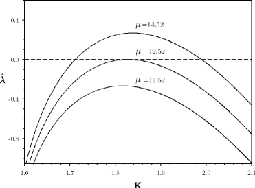
FIG. 1.: Dispersion relation $\widehat{\lambda}(K)$ for different values of the parameters ($\mu=\sqrt{rm}L_{1}^{2}/D$).

Now we propose a microscopic discrete stochastic formulation of the model which allows us to describe the role of demographic fluctuations. This implementation introduces two relevant differences. The first one is due to the role of intrinsic stochasticity which causes internal noise. The second one is specifically related to the discrete nature of individuals which can generate threshold effects not present in a continuum description where every small amount of the density of population is acceptable, an assumption of continuity which is often unrealistic (atto-fox problem [10]). Individual-based lattice models for similar Lotka-Volterra system have been studied in details in previous works [11, 12]. In general, the introduction of stochasticity generates a system considerably richer and perhaps even more realistic.

For the sake of simplicity our individual based model is implemented in a 1-dimensional system where the following algorithm was carried out. Simulations start with an initial population of $P_{0}$ predators and $N_{0}$ preys, randomly located along a ring (periodic boundary conditions) of length equal to $1$. The different processes of diffusion, reproduction and death are implemented sequentially by randomly selecting an individual of each population (predator or prey). The selected action is repeated for a number of times equal to the size of the corresponding population. When all the processes are carried out, a time step ends and the algorithm restarts. In detail, we are considering five processes: 1) diffusion, where a predator (prey) is randomly selected and moves some distance, in a random direction, chosen from a Gaussian distribution of standard deviation $\sigma$. 2) predator reproduction, with rate $\beta N^{x}_{L_{2}}$, where $N^{x}_{L_{2}}$ is the number of preys which are at a shorter distance than $L_{2}$ from the predator at position $x$. 3) predator death, with probability $m$. 4) prey reproduction, with probability $r$. 5) prey death, with rate $\alpha P^{y}_{L_{1}}$, where $P^{y}_{L_{1}}$ is the number of predators which are at a shorter distance than $L_{1}$ from the prey at position $y$. All the newborns maintain the same location as the parents. We evaluate $N^{x}_{L_{2}}$ and $P^{y}_{L_{1}}$ using periodic boundary conditions. If, in eq. LABEL:eq_1, we measure time in units of the simulation time step, the coefficient $D$ is related to the discrete model through $D=\sigma^{2}/2$. Birth and death probabilities are the same in the continuous and in the discrete model. A rigorous derivation which would show that the continuum field equations approximating the discrete model correspond to the eq. LABEL:eq_1, can be obtained by using Fock space techniques [8, 12].

The agent based simulations produced a rich collection of data which allow to explore the temporal and spacial behavior of our system. Irregular oscillations, which swing in a rather erratic fashion around an average value, characterize the temporal evolution (see Fig. 2). Other stochastic models display a similar behavior [11, 12]. There, inevitable fluctuations tend to push the system away from the trivial survival phase and induce irregular population oscillations that almost resemble the deterministic cycles of the classical Lotka-Volterra model. These features well approximate the temporal evolution of our simulations characterized by homogeneous spatial distributions. For example, the behavior of the dominant Fourier component displayed by the time evolution of these data depend only on the parameters $r$ and $m$, in a fashion consonant with a classical Lotka-Volterra system. Moreover, the presence of oscillations is independent of the population size, and therefore they persist in the thermodynamic limit [12]. The more the spatial solution is marked by clustering (lower $L_{1}$ and $D$ values), the more the irregularities of the temporal oscillations increase. Finally, we must remember that an important outcome of the introduction of intrinsic stochasticity is the possibility of predators’ extinction. For obviously, when the number of predators becomes very low, a chance fluctuation may lead the system into a state with $P(x,t)=0$. Therefore, asymptotically as $t\to\infty$ this state will be reached.

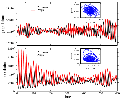
FIG. 2.: Temporal evolution. Top, populations with homogeneous spatial distributions ($L_{1}=L_{2}=0.1$). Bottom, populations with modulated spatial distributions ($L_{1}=0.05$, $L_{2}=0.1$). Others parameters are: $\sigma=0.004$, $r=m=0.5$, $\alpha=\beta=6.25\times 10^{-5}$, $P_{0}=N_{0}=40000$.

Now we turn to the analysis of the spatial aspects of the distributions of the populations. In accordance with the results of the continuous model no regular patterns can emerge for interactions characterized by the same range. For $L_{1}\neq L_{2}$, clear spatial patterns are generated (Fig. 3). For an interaction equal to the ring dimension, the simulation is characterized by a spatially homogeneous occupancy. Decreasing the $L_{1}$ value one peak appears, with the population concentrated in one region of the ring. For lower values of the interaction length, some regions of the ring are occupied forcing all the remaining areas, up to some range, to be nearly empty. This state corresponds to a sequence of isolated colonies (spikes) [8, 13]. We also observe that high population density can generate distributions where the colonies merge up, without loosing the ordered character of the modulation. We have deeply explored the case with $L_{1}=2L_{2}$. Even if $L_{1}\neq L_{2}$, the number of peaks is generally equal for predators and preys and the tuning of the parameter $L_{1}$ allows modulations of arbitrary wavelengths. Finally, for extremely short-ranged interaction, a noisy spatially homogeneous distribution appears (see Fig. 4). The reported periodic spatial patterns are stationary, with configurations characterized by a noise which increases in the neighborhood of the transition towards the homogeneous distribution. These outcomes obtained from simulations on the segment $(0,1)$ can be extended into a 2-dimensional space where fluctuating clusters arranged on an hexagonal lattice can emerge.

We can observe that for low $D$ values and low population density disordered spikes can appear, independently on the values of $L_{1}$, probably generated by the asymmetry between birth and death processes [14]. In fact, birth events only occur adjacent to a living organism, whereas deaths occur anywhere. This fact introduces a source of spatial correlation which can result in a reproductively driven cluster mechanism. Hence, under reproductive fluctuations and in the presence of a weak diffusion, individuals can organize into clusters. These inhomogeneous configurations can be related with the patterns observed in discrete lattice simulations, where spatial structures can also be generated by traveling waves [12, 15].

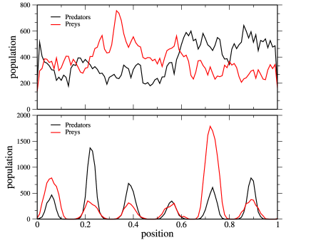
FIG. 3.: Spatial distributions. Top, homogeneous spatial distributions ( $L_{1}=L_{2}=0.1$). Bottom, modulated distributions ($L_{1}=0.05,L_{2}=0.1$). We can note preytaxis. Same parameters as in Fig. 2, t=600.

In the previous paragraph we show how inhomogeneous spatial distributions can appear, depending on the parameters value. Now, we will try to characterize the transition towards these states (segregation transition). A proper order parameter is provided by $q_{M}=\mathop{max}_{q>0}\Big{|}\sum\limits_{j=1}^{N(\tau)}\exp[i2\pi q\cdot x_{j}(\tau)]\Big{|}^{2}$, where the sum is performed over all individuals $j$ with their positions determined by $x_{j}$ at a given time $\tau$. The transition from a homogeneous to an inhomogeneous distribution matches the jump of $q_{M}$ to an integer value, corresponding to the number of periodic clusters present in the space. In fact, if the space is homogeneously occupied $q_{M}\simeq 1.4$ and the segregation transition is characterized by the passage of $q_{M}$ from $1.4$ to an integer value as soon as a modulation becomes dominant [13, 8]. In Fig. 4 we show $q_{M}$ as a function of $D$ and $L_{1}$. For any value of the range of the interaction, a critical value of the diffusion coefficient ($D_{c}$) exists above which no spatial structures emerge. For $r=m=0.5$ and $L_{1}=0.1$ the analytical prediction gives $D_{c}=4\times 10^{-4}$, in good accordance with the discrete model where the first set of simulations for which $q_{M}=1.4$ presents a diffusion coefficient equal to $D_{c}\approx 3.7\times 10^{-4}$. Moreover, a critical value of $L_{1}$ exists ($L_{c}$) for which the segregation transition takes place. For $L_{1}>L_{c}$ clusters appear and the value of $L_{c}$ obtained by the simulations is in accordance with the analytical result coming from eq. 6. Finally, another correspondence between the predictions of the continuous model and the Monte Carlo simulations exists. In fact, the continuous description can even reproduce quantitatively the period of the patterns in the modulated distributions. For example, considering the case displayed in Fig. 3, for $L_{1}=0.05$, the first relation in (6) tell us that the fastest growing mode is $k=36.6$. This is in good agreement with $6\times 2\pi=37.7$, which is the wavenumber of the configuration generated by our simulation. In fact, this wavenumber is the first immediately above the fastest growing mode of the mean-field description which is compatible with the periodic boundary conditions. For obvious, from the same equation in (6), we can obtain the general analytical relation for the number of peaks $n$: $n\approx 0.29L_{1}^{-1}$, which is compared with the Monte Carlo data in Fig. 4.

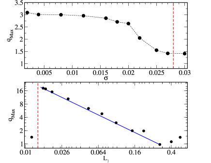
FIG. 4.: Top, $q_{M}$ as a function of $\sigma$ ($L_{1}=0.1$, $L_{2}=0.2$, $r=m=0.5$, $P_{0}=N_{0}=20000$). Data are averaged over $50$ realizations. The dashed line stands for the analytical result $\sigma_{c}\approx 0.028$. Bottom, log-log plot. $q_{M}$ as a function of $L_{1}$ ($L_{2}=2L_{1}$, $\sigma=0.004$, $r=m=0.5$, $P_{0}=N_{0}=40000$). Data are averaged over $20$ realizations. The continuous line represents the analytical prediction: $n\approx 0.29/L_{1}$. The dashed line stands for the analytical result $L_{c}\approx 0.014$. The structure functions are averaged over $20$ time steps, starting at $t=580$.

In conclusion, the introduction of a finite-range interaction in a spatial Lotka-Volterra model, allows the description of a rich spatio-temporal dynamics characterized by regular spatial structures. This type of spatial behavior is a central issue in population ecology as, effectively, it is possible to record spatial correlations between preys and predators in nature. Our investigation was carried out both analytically, using a suitable continuous model (mean-field approach), as well with a discrete model, by employing Monte Carlo simulations. The individual-based model shows the existence of spatial structures in an erratic oscillatory regime which can contemplate predators’ extinction. The mean-field description captures the essential features of the discrete model. We record quantitative correspondences for the period of the spatial patterns in the modulated distributions, the value of the critical diffusion and the critical interaction length. From an ecological perspective, the emergence of spatial patterns in an erratic oscillatory regime are realistic elements generally absent from conventional approaches and might shed further light on issues of particular ecological relevance.

We thank the Brazilian agencies CNPq for partial financial support and the school CSSS 2008, of the Santa Fé Institute, where this work was conceived. We are grateful to B. Perthame for helpful discussions.

REFERENCES

- [1] P.A.P. Moran, Aust. J. Zool. 1, 291 (1953); W.D. Koenig, Trends Ecol. Evol., 14, 22, (1999)
- [2] J. Bascompte and R.V. Solé, Trends Ecol. Evol., 10, 361, (1995); O.N. Bjørnstad, R.A. Ims and X. Lambin, Trends Ecol. Evol., 14, 427, (1999).
- [3] P.C. Tobin and O.N. Bjørnstad, J. Anim. Ecol., 72, 460 (2003).
- [4] J.D. Murray, Mathematical Biology, Springer (1989).
- [5] E.E. Holmes, M.A. Lewis, J.E. Banks and R.R.Veit, Ecology 75, 17 (1994); D. Alonso, F. Bartumeus and J. Catalan, Ecology, 83, 28, (2002).
- [6] R. MacArthur, and R. Levins, Am. Nat., 101, 377 (1967); J. Roughgarden, Theory of Population Genetics and Evolutionary Ecology: an Introduction. Macmillan Publishers (1979); M. A. Fuentes, M. N. Kuperman, and V. M. Kenkre, Phys. Rev. Lett. 91, 158104 (2003); P. Szabó and G. Meszéna, Oikos 112, 612 (2006); M. Scheffer, E.H. Van Nes, Proc. Natl. Acad. Sci. USA, 103, 6230 (2006).
- [7] F. Bagnoli and M. Bezzi, Phys. Rev. Lett. 79 3302 (1997); U. Dieckmann and M. Doebeli, Nature 400, 354 (1999); V. Schwämmle and E. Brigatti, Europhys. Lett. 75, 342 (2006); E. Brigatti, J. S. Sá Martins and I. Roditi, Physica A 376, 378 (2007).
- [8] E. Hernandez-Garcia and C. Lopez, Phys. Rev. E 70, 016216 (2004).
- [9] B. Perthame and S. Génieys, Math. Model. Nat. Phenom. 4, 135, (2007).
- [10] D. Mollison, Mathematical Biosciences 107, 255 (1991).
- [11] W.G. Wilson, A.M. De Roos, and E. McCauley, Theoretical Population Biology, 43, 91 (1993); J. E. Satulovsky and T. Tomé, Phys. Rev. E 49, 5073 (1994); A. Provata, G. Nicolis and F. Baras, J. Chem. Phys. 110, 8361 (1999); A. Lipowski, Phys. Rev. E 60, 5179 (1999).
- [12] M. Mobilia, I. T. Georgiev and U. C. Tauber, J. Stat. Phys., 128, 447 (2007).
- [13] E. Brigatti,V. Schwämmle, and M.A. Neto, Phys. Rev. E 77, 021914 (2008).
- [14] W. R. Young, A. J. Roberts and G. Stuhne, Nature 412, 328 (2001).
- [15] M. Roy, M. Pascual, and A. Franc, Complexity, 8, 19 (2003).