Four Generations: susy and susy Breaking

Rohini M. Godbole, Sudhir K. Vempati, Akın Wingerter

Centre for High Energy Physics,

Indian Institute of Science, Bangalore 560012, India

Abstract

We revisit four generations within the context of supersymmetry. We compute the perturbativity limits for the fourth generation Yukawa couplings and show that if the masses of the fourth generation lie within reasonable limits of their present experimental lower bounds, it is possible to have perturbativity only up to scales around 1000 TeV. Such low scales are ideally suited to incorporate gauge mediated supersymmetry breaking, where the mediation scale can be as low as 10-20 TeV. The minimal messenger model, however, is highly constrained. While lack of electroweak symmetry breaking rules out a large part of the parameter space, a small region exists, where the fourth generation stau is tachyonic. General gauge mediation with its broader set of boundary conditions is better suited to accommodate the fourth generation.

1 Introduction

Interest in a sequential fourth generation of chiral fermions has waxed and waned over the past decades with the changing status of constraints implied by various precision measurements in the flavour and the gauge sector. The recent observation of single-top events at the Tevatron [1, 2] allowed a direct and clean determination of the CKM matrix element $|V_{tb}|=0.91\pm 0.11\,\text{(stat+syst)}\pm 0.07\,\text{(theory)}$ [2]. This is in good agreement with the Standard Model prediction of $|V_{tb}|\simeq 1$, but falls short of excluding extensions of the theory by another chiral generation of quarks and leptons, as has been emphasised in recent publications [3, 4, 5, 6, 7, 8]. As a matter of fact, the mixing between the third and a hypothetical fourth family can be as large as the mixing between the first two generations in the Standard Model and yet be compatible with all experimental data including direct searches for new quarks and leptons, electroweak precision measurements, and flavour changing neutral currents [9, 5, 6, 4, 8].

Currently, we do not have a theoretical understanding of the number of generations, and a priori there is no reason why there should not be another one. A fourth generation would have profound implications for particle physics phenomenology. For one thing, it can ease the tension between the LEP bound on the Higgs mass and the electroweak precision measurements [4, 6, 8] as we will elaborate on in Section 2. Secondly, the Yukawa couplings of the fourth generation fermions, heavier than those of the first three, will have important implications for the perturbativity of the theory at the high scale. This can have nontrivial effects, for example, on the Higgs mass bounds obtained in the SM by demanding that the Landau pole lie above the Planck scale [11, 12]. As a result of this possible effect of the fourth generation on the consistency of the theory up to high scale, unified theories with four generations have also received special attention, both with supersymmetry (SUSY) [13, 14, 15, 16, 17, 18, 19, 20] and without it [21]. The fourth generation can also account for the extra CP violation needed for electroweak baryogenesis to work [22, 23, 24]. Other ideas that have been explored in connection with four generations include: Extra dimensions [25, 26, 27], technicolour [28, 29, 30] and electroweak symmetry breaking [31, 32, 33], radiative mass generation [34, 35], bounds from cosmology [36], neutrino physics [37, 38, 39], and finally string theory [40].

Recent analyses of the fourth generation have mainly focused on the the non-supersymmetric case. In this, we extend the minimal supersymmetric standard model (MSSM) by one chiral generation and explore the implications for supersymmetry and supersymmetry breaking. For clarity, we will call the MSSM with three and four generations MSSM3 and MSSM4, respectively. In Section 2, we review the constraints on the masses of the fourth generation coming from experiment, precision electroweak data, and flavour changing neutral currents. In Section 3, we introduce our notation and map out the parameter space of the MSSM4 where the theory remains perturbative up to some assumed unification scale of the order $2\times 10^{16}$ GeV. We will find that this puts severe restrictions on $m_{t^{\prime}}$, $m_{b^{\prime}}$, $m_{\tau^{\prime}}$, $\tan\beta$, and show that the current experimental bounds and perturbative unification are mutually exclusive. Depending on the masses and $\tan\beta$, the theory becomes strongly-coupled around 10-1000 TeV. To illustrate the qualitative differences, we will present a toy mSUGRA model where we have chosen the quark and lepton masses to be equal to their third generation counterparts. In Section 4, motivated by the low “perturbativity” scale, we explore this issue in the context of gauge mediated supersymmetry breaking (GMSB). Minimal GMSB, however, suffers from tachyons in the spectrum, and hence we are led to generalise our GMSB set-up in the quest for realistic models. Finally, in Section 5 we summarise our results and outline directions for future work.

2 Limits from Experiment, Electroweak Precision Data, and FCNC

The current experimental limits quoted by the PDG [41] at 95% CL are :

$$m_{t^{\prime}}\gtrsim 256\text{ GeV,}\quad m_{b^{\prime}}\gtrsim 128\text{ GeV,}\quad m_{\tau^{\prime}}\gtrsim 100.8\text{ GeV,}\quad m_{\nu_{\tau}^{\prime}}\gtrsim 45\text{ GeV.}$$ (1)

The bounds on $m_{t^{\prime}}$ and $m_{b^{\prime}}$ assume that the predominant decay mode is to a $W$ boson and another quark [42, 43], which we expect to be true for a sequential fourth generation. Along the same lines, for the limit on $m_{\tau^{\prime}}$ one assumes that $\tau^{\prime}$ decays to a $W$ and a stable $\nu_{\tau}^{\prime}$ [46], and the limits for a stable heavy neutral particle give the lower bound on $m_{\nu_{\tau}^{\prime}}$ [47].

Electroweak precision measurements further constrain the allowed mass ranges. For no mixing between the third and fourth generation, $\chi^{2}$ is minimised for $|m_{t^{\prime}}-m_{b^{\prime}}|\simeq 45-75$ GeV [4], and for $m_{t^{\prime}}=300$ GeV with $m_{b^{\prime}}$ subject to this constraint, the mixing can be as large as $\sin\theta_{34}=0.35$ [6]. The precision data excludes larger mixing between the third and fourth families [6] that is otherwise allowed from FCNC constraints [5].

Fig. 10.4 of Ref. [41] by the PDG shows the constraints from electroweak precision measurements. The values $S=-0.04\pm 0.09$ and $T=0.02\pm 0.09$ obtained from the fit are in best agreement with a Higgs mass of $m_{H}=117$ GeV. For higher Higgs masses, the 90% CL contours move towards smaller $S$ and larger $T$ values. From this it is clear that a fourth generation may ease the tension between the LEP bound on the Higgs mass and the electroweak precision data, since its contribution to $T$ is typically positive [4, 6]. A fourth generation can give a negative contribution to $S$, but the mass splitting of the quarks is constrained by the $T$ parameter and leads to a positive correction to $S$ that has to be kept small in order to stay in the 90% CL ellipse.

Note that the limits quoted in 1 are at 95$\%$ CL. In the absence of direct availability of these bounds at a higher level of confidence, we approximate them by subtracting 20% off the respective limits at 95$\%$ CL. Furthermore, the exclusion limits denote the pole masses, whereas in our calculations, we need to use the running masses. We will account for this difference by taking yet another 5% off the masses for QCD corrections. Note that this is a conservative estimate as the SUSY threshold corrections can induce an additional difference up to 20% between the pole and the running masses [48].

In our analysis, we will thus be working with two sets of mass limits, namely those at $95\%$ CL as well as the weaker lower bounds obtained with the above-mentioned prescription. Both sets are subject to the constraint from electroweak precision measurements that the mass splitting in the same SU(2) multiplet be not greater than $\sim$ 75 GeV. Thus we consider in our analysis the following sets of fourth generation fermion masses:

$$m_{t^{\prime}}=256\text{ GeV,}\quad m_{b^{\prime}}=181\text{ GeV,}\quad m_{\tau^{\prime}}=100.8\text{ GeV}$$ (2)

$$m_{t^{\prime}}=192\text{ GeV,}\quad m_{b^{\prime}}=117\text{ GeV,}\quad m_{\tau^{\prime}}=\phantom{1.8}75\text{ GeV}$$ (3)

We will comment on the mass of the fourth generation neutrino in Section 3.

3 Perturbativity and Four Generations

One of the main constraints in considering models with four generations is the perturbativity of the Yukawa couplings. With the masses of the fourth generation expected to be typically larger than the already known third generation masses, the scale up to which the theory remains perturbative is a major concern. It is expected that supersymmetry would soften the running of the Yukawa couplings and enable the theory to be valid up to much higher energy scales. It is well known that the Yukawa couplings of the heavy fermions flow under the renormalisation group to a infrared (quasi-)fixed point. The proximity of the observed top mass to this limit (see e.g. Ref. [49]), in fact also indicates that a fourth generation of fermions, heavier than the top quark, can have important implications for the high scale perturbativity of the theory.

In the present section, we discuss this issue in detail and present the results of our computations. As we will show, these high scales will extend only up to $\sim$ 1000 TeV. Let us also note that in supersymmetric theories the scale up to which perturbativity is preserved has implications for (a) gauge coupling unification and (b) the scale of supersymmetry breaking, though a priori they are two independent sectors of the theory.

The generalisation of the MSSM to four generations is straight-forward. We will denote the fourth generation as the primed generation: ($t^{\prime},b^{\prime},\tau^{\prime},\nu_{\tau}^{\prime}$) and denote this model as MSSM4. The standard MSSM picture with three generations will from now on be mentioned as MSSM3. The MSSM4 superpotential takes the form :

$$W=u^{c}~{}\mathbf{Y_{u}}QH_{2}+d^{c}~{}\mathbf{Y_{d}}QH_{1}+e^{c}~{}\mathbf{Y_{e}}LH_{1}+\mu H_{1}H_{2},$$ (4)

where $\mathbf{Y}$ are $4\times 4$ matrices in generation space. The Yukawa couplings of the fourth generation, defined in terms of their masses, are given as

$$h_{t^{\prime}}=~{}{m_{t^{\prime}}\sqrt{2}\over v\sin\beta}\;\;,\;\;h_{b^{\prime}}=~{}{m_{b^{\prime}}\sqrt{2}\over v\cos\beta}\;\;,\;\;h_{\tau^{\prime}}=~{}{m_{\tau^{\prime}}\sqrt{2}\over v\cos\beta},$$ (5)

where $v=246$ GeV stands for the Higgs vacuum expectation value.

In addition, the fourth generation neutrino $\nu_{\tau^{\prime}}$ should also attain a mass $m_{\nu_{\tau}^{\prime}}~{}>45$ GeV. There are several ways of generating the fourth generation neutrino mass term , which may either be of the Dirac type or a mixture of Dirac plus Majorana type, leading to a Majorana mass for the $\nu_{\tau^{\prime}}$ and this can make the analysis highly model dependent. In the present case, we have not considered the effects of a Dirac Yukawa coupling for the neutrino in the renormalisation group equations (RGE). It should be noted that a large neutrino Dirac Yukawa coupling can, in principle, affect strongly the evolution of the Yukawa coupling of the $\tau^{\prime}$ but, the effect would be minimal as long as the said neutrino Dirac Yukawa coupling is small. A more detailed analysis of the various possible neutrino Yukawa couplings and their impact on perturbativity will be presented elsewhere.

Firstly, let us note that the larger masses of the down type fourth generation fermions mean that requiring that the Yukawa couplings be perturbative at the weak scale puts upper bounds on tan $\beta$, stronger than the ones present in the MSSM3. The strongest limit comes from $h_{b^{\prime}}$. Imposing that $h_{b^{\prime}}^{2}\sim 4\pi$, we have :

$$\tan\beta\leq\left(2\pi\left({v\big{/}m_{b^{\prime}}}\right)^{2}-1\right)^{1\over 2}$$ (6)

For the lower limit of $m_{b^{\prime}}$ quoted in 2 this already sets a limit $\tan\beta~{}\leq$ 4.7. The bound from $m_{\tau^{\prime}}$ is much weaker, $\tan\beta\sim$ 38. Even for the values of $\tan\beta$ obeying this limit, the Yukawa couplings are not expected to be perturbative all the way up to the GUT scale, where the gauge coupling unification happens.

It should be noted that in the presence of four generations, gauge coupling unification at the 1-loop level still takes place at the scale $M_{\text{GUT}}\sim 2\times 10^{16}$ GeV, though the value of $\alpha_{\textsc{gut}}$ itself changes. We refer to Appendix A.1 for the relevant renormalisation group equations. At the 2-loop level, the renormalisation group running of gauge couplings will involve Yukawa couplings and thus if the Yukawa couplings become non-perturbative at scales much lower than $M_{\textsc{gut}}{}$ they could render the same to the gauge couplings. In the non-supersymmetric Standard Model with four generations, it has been known that perturbative unification of the gauge couplings is possible [21]. However, the values for the fourth generation masses used in the analysis of Ref. [21] are ruled by the recent experimental results (see also Ref. [12]).

In the following, we will derive upper limits on the fourth generation fermion masses by requiring that the Yukawa couplings of the fourth generation be perturbative all the way up to the GUT scale.

For this purpose, we use the two loop RGE equations listed in Appendix A.2 for $n_{G}$ number of generations. Needless to say, $n_{G}=3$ for MSSM3 and $n_{G}=4$ for MSSM4. We solve these equations numerically for a given set of masses at the weak scale and check whether the corresponding Yukawa couplings remain perturbative at the high scale.

We have developed a variant of the popular supersymmetric spectrum calculator, SOFTSUSY [50], called INDISOFT. It contains significant modifications including the ability to handle three or four generations. Some technical aspects are presented in the Appendix B.

We first vary $m_{t^{\prime}}$ and $m_{b^{\prime}}$ while keeping $m_{\tau^{\prime}}$ fixed and later vary $m_{b^{\prime}}$ and $m_{\tau^{\prime}}$ while keeping $m_{t^{\prime}}$ fixed. From the RGE in Appendix A.2 we see that the evolution of $t^{\prime}$ is independent of the $\tau^{\prime}$ mass at 1-loop order. With this in mind, for the first analysis we take the $\tau^{\prime}$ mass to be negligible. For numerical purposes we set it equal to the $\tau$ mass, i.e. $m_{\tau^{\prime}}~{}=m_{\tau}$. Before presenting the numerical results one final comment is in order. The Yukawa couplings of the heavy fields (e.g. $t^{\prime}$, $t$) flow towards an infrared fixed point at the weak scale. Using this one can derive an upper bound on these masses of the heavy fermions analytically. The analytical results for the $t^{\prime}$ are presented in Appendix A.3.

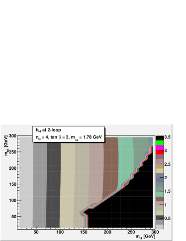
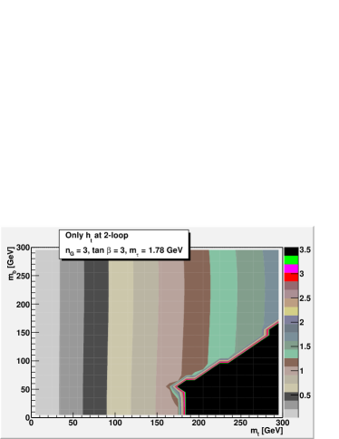
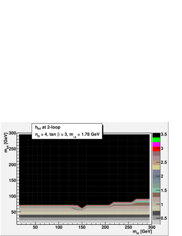
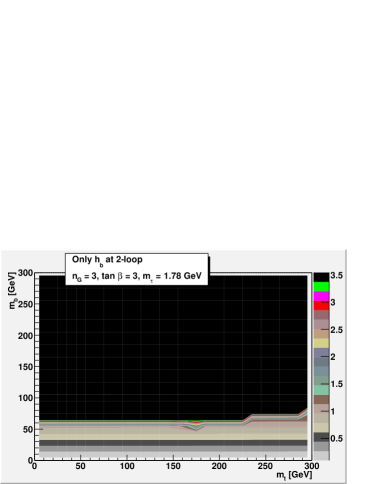
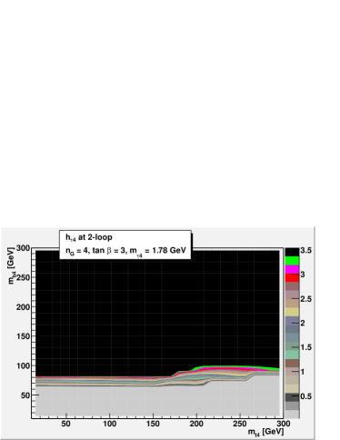
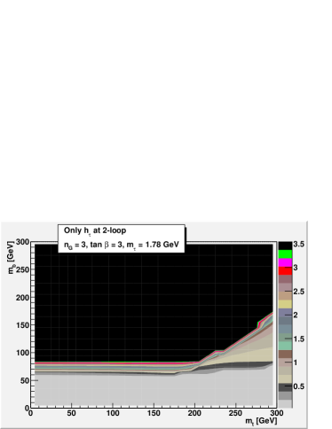
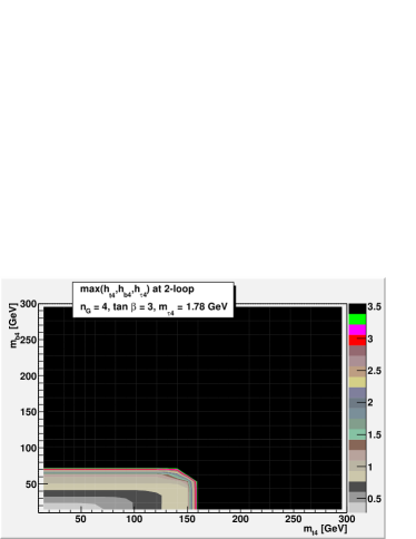
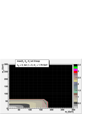
Figure 1: The first three rows of the left and right panels show $h_{t^{\prime}}$, $h_{b^{\prime}}$, $h_{\tau^{\prime}}$ in MSSM4, and $h_{t}$, $h_{b}$, $h_{\tau}$ in MSSM3, respectively, at 2-loop and $M_{X}=2.3\times 10^{16}$ GeV, plotted in the $m_{t^{\prime}}$–$m_{b^{\prime}}$ and $m_{t}$–$m_{b}$ plane for $\tan\beta=3$ and $m_{\tau^{\prime}}=m_{\tau}=1.78$ GeV. For the MSSM4 case this experimentally excluded value is chosen for illustrative purposes only. The black regions indicate where the Yukawa couplings become non-perturbative. The last row shows the regions where all Yukawa couplings are perturbative.

In the left column of 1, we plot the regions in the $m_{b^{\prime}}-m_{t^{\prime}}$ plane where the Yukawa couplings remain perturbative all the way up to the GUT scale using 2-loop MSSM4 RGE. We have chosen $\tan\beta=3$. In the first row, the condition that only the top-prime Yukawa coupling remains perturbative all the way is plotted. The perturbativity limit is taken to be $\sqrt{4\pi}\simeq 3.54$. All the regions are colour-coded with the values that the Yukawa couplings take at the high scale. The legend for the colour-coding is shown on the right side of each plot. If the Yukawa coupling attains a value beyond the upper limit of $3.54$, the point is flagged as non-perturbative and is denoted in black. Thus, in each of these plots regions in black are ruled out by the perturbativity limit. From this first plot of the left column, we see that a large region in $m_{t^{\prime}}$ opens up as the $b^{\prime}$ mass increases. For $m_{b^{\prime}}>70$ GeV, $m_{t^{\prime}}>150$ also can be made valid. However, although the $t^{\prime}$ Yukawa coupling is perturbative in these regions, the other two Yukawa couplings are not, as is evident from the plots in the next two rows. In the second row, left column, we exhibit the same plots, however requiring that only $h_{b^{\prime}}$ remains perturbative, and in the third row, left column, requiring that only $h_{\tau^{\prime}}$ remains perturbative. As we see from the plots, although the $t^{\prime}$ Yukawa coupling is perturbative, the $b^{\prime}$ and $\tau^{\prime}$ Yukawa couplings are no longer perturbative in these regions. The last row shows plots where all the constraints are put together. Here we see that for a negligible $\tau^{\prime}$ mass ($\sim$ 1.75 GeV), $t^{\prime}$ and $b^{\prime}$ masses are constrained to be:

$$0\lesssim m_{b^{\prime}}\lesssim 70\text{ GeV},\quad 0\lesssim m_{t^{\prime}}\lesssim 160\text{ GeV},\quad m_{\tau^{\prime}}=1.78\text{ GeV},\quad\tan\beta=3.$$ (7)

It is instructive to compare the above results with those of the MSSM3. In MSSM3, as we know, the Yukawa couplings do remain perturbative all the way up to the GUT scale for the known masses of the top and bottom quarks and the tau lepton, the only exception being in regions where $\tan\beta$ is very small or very large. In the right panel of 1, we present the analogous analysis for the case of the MSSM3. We have fixed the $\tau$ mass at its experimental value but varied $m_{t}$ and $m_{b}$. We have further fixed $\tan\beta$ to be 3 as in the case of four generations. The results in the case of MSSM3 are strikingly similar to those obtained for the four generational MSSM4. In fact we can read off from the plot the regions in $m_{t}-m_{b}$ plane where all the three Yukawa couplings remain perturbative:

$$0\lesssim m_{b}\lesssim 60\text{ GeV},\quad 0\lesssim m_{t}\lesssim 180\text{ GeV},\quad\tan\beta=3.$$ (8)

The reason for these similar results is the way Landau poles appear in the Yukawa couplings. The evolution of the Yukawa couplings depends only on themselves and the gauge couplings. As it is clear from the RGEs (see Appendix A.3), the evolution of the gauge couplings is very similar to that of the three generation case, except for the $\beta$-functions $b_{i}$ which change the slope of the $h(t)$. The change in the $b_{i}$ for the three vs. four generations is not very large to induce large changes in the upper limits. The difference is within a few tens of GeV.

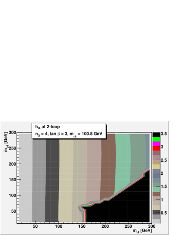
(a) Constraints in the $m_{b^{\prime}}$–$m_{t^{\prime}}$ plane from the perturbativity of $h_{t^{\prime}}$ for fixed values of $m_{\tau^{\prime}}=100.8$ GeV and $\tan\beta=3$.

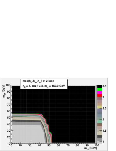
(b) Constraints in the $m_{b^{\prime}}$–$m_{\tau^{\prime}}$ plane from the perturbativity of the max $(h_{t^{\prime}},h_{b^{\prime}},h_{\tau^{\prime}}$), for fixed values of $m_{t^{\prime}}=150$ GeV and $\tan\beta=3$.

Figure 2: MSSM with 4 generations at 2-loop. The black region is where the respective Yukawa couplings become non-perturbative below the unification scale $M_{X}=2.3\times 10^{16}$ GeV.

The results of 7 are valid only when $m_{\tau^{\prime}}=m_{\tau}$. Increasing the value of $m_{\tau^{\prime}}$ to the lower limit of 2 significantly modifies these results. We find that as expected $m_{t^{\prime}}$ which is less dependent on the $\tau^{\prime}$ mass remains perturbative for a similarly large region of the parameter space as shown in 22(a). However, for the values,

$$0\lesssim m_{b^{\prime}}\lesssim 0~{}\text{ GeV},\quad 0\lesssim m_{t^{\prime}}\lesssim 160~{}\text{ GeV},\quad m_{\tau^{\prime}}=100.8~{}\text{ GeV},\quad\tan\beta=3,$$ (9)

$h_{b^{\prime}}$ is not perturbative for any $m_{b^{\prime}}$. In fact, $h_{\tau^{\prime}}$ itself is no longer perturbative.

We now proceed to keeping $m_{t^{\prime}}$ fixed while varying $m_{b^{\prime}}$ and $m_{\tau^{\prime}}$. We have chosen two values of $m_{t^{\prime}}$, the one given by the approximate perturbative upper limit $\sim 150$ GeV (7) and the other the experimental lower limit of 256 GeV. In 22(b), we have plotted the regions in the $m_{b^{\prime}}-m_{\tau^{\prime}}$ plane in which the theory remains perturbative all the way up to the GUT scale. From the figure we can read off the valid mass ranges as:

$$0\lesssim m_{b^{\prime}}\lesssim 60~{}\text{ GeV},\quad 0\lesssim m_{\tau^{\prime}}\lesssim 50~{}\text{ GeV},\quad\tan\beta=3,\quad m_{t^{\prime}}=150\text{ GeV}$$ (10)

$$0\lesssim m_{b^{\prime}}\lesssim 56\text{ GeV},\quad 0\lesssim m_{\tau^{\prime}}\lesssim 53\text{ GeV},\quad\tan\beta=3,\quad m_{t^{\prime}}=256\text{ GeV}$$ (11)

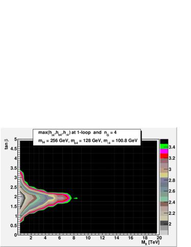
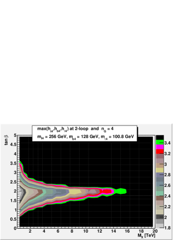
(a) For the masses in 1 without $T$-parameter constraints.

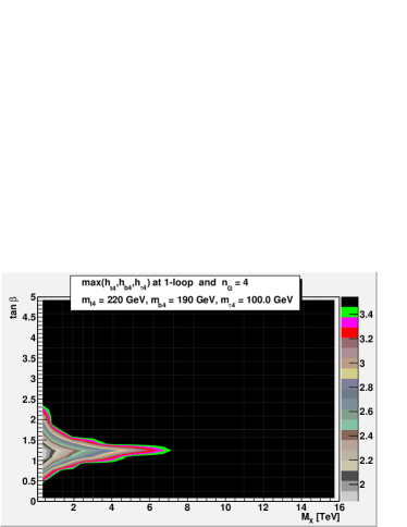
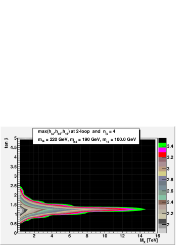
(b) For the masses considered in Ref. [20].

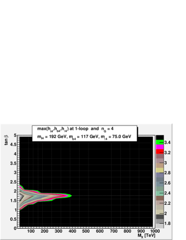
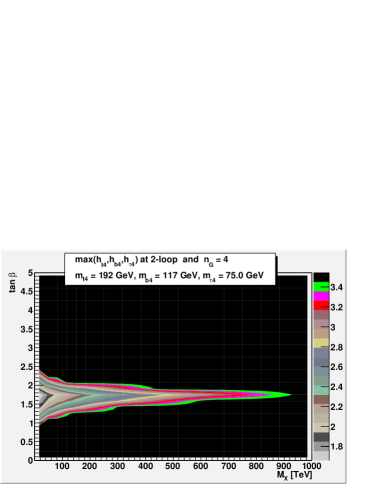
(c) For the masses in 3 with $T$-parameter constraints.

Figure 3: Regions in the $M_{X}$–$\tan\beta$ plane where all the Yukawa couplings of the charged fourth generation fermions are perturbative at 1-loop and 2-loops respectively. The different rows correspond to different values of the fermions indicated on the panels and explained in the subcaption of the figure in each row.

Clearly these mass ranges are excluded by the constraints of 1 or even by the weaker constraints in 2 and 3 on page 3.

To restore the perturbativity in the theory we can take either of the two approaches (i) add new particles with new Yukawa contributions so as the keep the Yukawa couplings perturbative all the way up to the GUT scale (ii) take the view point that the theory is valid only up to a scale which is allowed by perturbative constraints and then some new non-perturbative physics takes over. We will study the second option in the present work and note that the first option has already been considered by others. To this end, we do a complete scan of the allowed regions of the high scale, $M_{X}$, and $\tan\beta$ for a given set of values of $m_{t^{\prime}},m_{b^{\prime}},m_{\tau^{\prime}}$. In 3, we present the results using the lower limits on the fourth generation masses given in 2 and 3 on page 3. We have demanded that all the Yukawa couplings remain perturbative up to the scale $M_{X}$. We have presented the results using both 1-loop as well as 2-loop RGE to show the importance of using 2-loop RGE. From the 1-loop plot we see that for $\tan\beta\sim 2$, the Yukawa couplings barely remain perturbative up to 8 TeV or so. At the two loop level this scale increases to about 16 TeV.

We have also compared our analysis with that of Ref. [20]. We have chosen the same masses $m_{t^{\prime}}=220$ GeV, $m_{b^{\prime}}=190$ GeV and $m_{\tau^{\prime}}=100$ GeV. The allowed regions in $M_{X}$ vs. $\tan\beta$ plane are presented in 33(b) on page 3. We find that while qualitatively we agree with them, quantitatively we differ in the maximal value of $M_{X}$ by a couple of orders in magnitude.

33(c) on page 3 shows that if we choose the fourth generation fermion masses to be at the weaker lower limits (see 3), we can have perturbativity all the way up to $\sim$ 1000 TeV. Note that these weaker lower limits are obtained under very reasonable assumptions. Finally, the relevant $M_{X}$ and $\tan\beta$ ranges can be read out from the plots as follows :

$$1\lesssim\tan\beta\lesssim 3.6,\quad 1\text{ TeV}\lesssim M_{X} \lesssim 16\text{ \enspace TeV}\quad\text{for \ref{pdglimits} on page \ref{pdglimits}}$$

$$1\lesssim\tan\beta\lesssim 2.4,\quad 1\text{ TeV}\lesssim M_{X} \lesssim 920\text{ TeV}\quad\text{for \ref{ourlimits} on page \ref{ourlimits} }$$ (12)

3.1 Implications for mSUGRA

Before closing this section, let us comment on the possibility of realising minimal supergravity with four generations. From a phenomenological point of view such a possibility would be interesting with supersymmetric partners of the fourth generations leading to new experimental signatures at the weak scale. Further, due to the presence of additional Yukawa couplings, the weak scale supersymmetric mass spectrum would most likely be quite different from that of mSUGRA3 [18]. If the fourth family Yukawa couplings are large, they could contribute significantly to the lightest Higgs mass at the 1-loop level, thus alleviating the little hierarchy problem [23], [51]. However, in the standard picture of mSUGRA with universal or non-universal soft masses at the GUT scale, radiative electroweak symmetry breaking induced by the large $t^{\prime}$ (and possibly $b^{\prime},\tau^{\prime}$) Yukawa coupling and the neutralino as the lightest supersymmetric particle, would require the theory to remain perturbative all the way up to the GUT scale. From the analysis above, we see that theory would remain perturbative with four generations only if the fourth generation masses are much lower than their experimental lower limits, in fact, closer to the third generation masses. In the following we will consider a toy model of mSUGRA4, where the masses of the fourth generation are set equal to the their third generation counterparts:

$$m_{t^{\prime}}=m_{t},\quad m_{b^{\prime}}=m_{b},\quad m_{\tau^{\prime}}=m_{\tau}.$$

We then compute the mass spectrum at the weak scale for a sample point and compare it with that of mSUGRA3. We use our new tool INDISOFT to compute the spectrum at the weak scale.

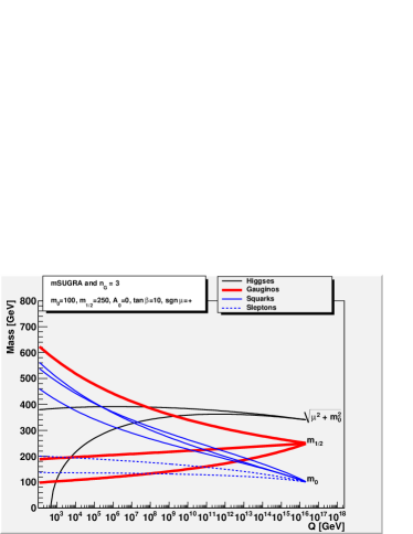
(a) Three generations.

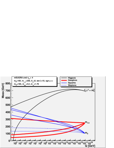
(b) Four generations.

Figure 4: The running of the various soft masses in the MSSM3 and MSSM4 is shown in the left and right panel, respectively. The legend is indicated in the panel. The Higgses are the black lines starting at $\sqrt{\mu^{2}+m_{0}^{2}}$.

The very presence of four generations, irrespective of whether their Yukawa couplings are large or not, can lead to interesting differences between the three and four generation RG evolution of the soft masses. In 4 we show the running patterns of the soft terms for three as well as four generations. As expected, the Higgs mass terms (black line) run to more negative regions as compared to three generation case, and in fact, they can both become negative even for small $\tan\beta$ in the four generation case. Perhaps the most interesting aspect is the running of the gluino mass, which now due to a smaller $\beta$-function, almost does not evolve (up to 1-loop level) in the four generation case (thick red line). The sleptons (dashed-blue) are not significantly affected, however the squarks (undashed-blue) run to lighter values due to reduced gluino running effects. All these differences in the running of the soft terms would make themselves evident in the mass spectrum at the weak scale.

Higgses [GeV]				Gauginos [GeV]				Squarks & Sleptons [GeV]
	$h^{0}$	106.7			$\widetilde{\chi}^{0}_{1}$	96.6		$\widetilde{u}_{L}$	568.2		$\widetilde{t}_{1}$	587.4
	$A^{0}$	382.2			$\widetilde{\chi}^{0}_{2}$	178.3		$\widetilde{u}_{R}$	547.5		$\widetilde{t}_{2}$	411.0
	$H^{0}$	382.6			$\widetilde{\chi}^{0}_{3}$	343.0		$\widetilde{d}_{L}$	573.6		$\widetilde{b}_{1}$	519.9
	$H^{\pm}$	390.9			$\widetilde{\chi}^{0}_{4}$	362.8		$\widetilde{d}_{R}$	546.6		$\widetilde{b}_{2}$	547.2
					$\widetilde{\chi}^{\pm}_{1}$	178.0		$\widetilde{e}_{L}$	205.7		$\widetilde{\tau}_{1}$	209.1
					$\widetilde{\chi}^{\pm}_{2}$	364.5		$\widetilde{e}_{R}$	146.7		$\widetilde{\tau}_{2}$	138.9
					$\widetilde{g}$	607.0		$\widetilde{\nu}_{e}$	189.8		$\widetilde{\nu}_{\tau}$	189.1

Table 1: MSSM spectrum with 3 generations and mSUGRA boundary conditions: $m_{0}=100$ GeV, $m_{1/2}=250$ GeV, $A_{0}=0$ GeV, $\tan\beta=10$, $\text{sgn\,}\mu$=+. The unification scale is $M_{\textsc{gut}}{}=2.40\times 10^{16}$ GeV.

Higgses [GeV]				Gauginos [GeV]				Squarks & Sleptons [GeV]
	$h^{0}$	119.5			$\widetilde{\chi}^{0}_{1}$	44.1		$\widetilde{u}_{L}$	480.4	$\widetilde{t}_{1}$	499.7	$\widetilde{t}_{1}^{\prime}$	498.8
	$A^{0}$	486.5			$\widetilde{\chi}^{0}_{2}$	83.4		$\widetilde{u}_{R}$	462.6	$\widetilde{t}_{2}$	357.8	$\widetilde{t}_{2}^{\prime}$	356.4
	$H^{0}$	486.2			$\widetilde{\chi}^{0}_{3}$	474.2		$\widetilde{d}_{L}$	486.7	$\widetilde{b}_{1}$	432.4	$\widetilde{b}_{1}^{\prime}$	428.7
	$H^{\pm}$	492.8			$\widetilde{\chi}^{0}_{4}$	478.1		$\widetilde{d}_{R}$	462.0	$\widetilde{b}_{2}$	465.9	$\widetilde{b}_{2}^{\prime}$	466.2
					$\widetilde{\chi}^{\pm}_{1}$	83.4		$\widetilde{e}_{L}$	187.7	$\widetilde{\tau}_{1}$	196.4	$\widetilde{\tau}_{1}^{\prime}$	196.2
					$\widetilde{\chi}^{\pm}_{2}$	481.4		$\widetilde{e}_{R}$	142.0	$\widetilde{\tau}_{2}$	126.5	$\widetilde{\tau}_{2}^{\prime}$	127.1
					$\widetilde{g}$	352.1		$\widetilde{\nu}_{e}$	170.4	$\widetilde{\nu}_{\tau}$	169.6	$\widetilde{\nu}_{\tau}^{\prime}$	169.6

Table 2: MSSM spectrum with 4 generations and mSUGRA boundary conditions: $m_{0}=100$ GeV, $m_{1/2}=250$ GeV, $A_{0}=0$ GeV, $\tan\beta=10$, $\text{sgn\,}\mu$=+. For the theory to be perturbative, we have chosen all 4th generation masses to be equal to their 3rd generation counterparts (toy model). The unification scale is $M_{\textsc{gut}}{}=8.82\times 10^{16}$ GeV.

In 1 and 2, we present the weak scale spectrum for some sample point. Comparing the spectrum in the two tables, we find the following: (a) the Higgs mass is heavier in mSUGRA4, in fact above the LEP limit (b) the lighter neutralinos in mSUGRA4 are lighter compared to mSUGRA3, with one close to 60 GeV (c) the squark and the gluino masses are also significantly lighter compared to mSUGRA3 (d) slepton masses do not have much of an impact and they seem to be close to those in mSUGRA3.

Thus the addition of a fourth chiral generation to MSSM3 seems to give rise to a lighter supersymmetric spectrum at the weak scale with a less fine tuned Higgs mass. These results, though valid only in this particular toy model, seem to indicate the possible features the supersymmetric spectrum would have if one could make theory perturbative. As discussed earlier, one possible way would be to add additional vector-like matter [20]. An alternative approach, which we follow, is to lower the scale of supersymmetry breaking and ask whether the above features are replicated. We thus look for a low scale supersymmetry mediation mechanism which is preferably close to the non-perturbative regime in the Yukawa couplings.

4 GMSB with Four generations

4.1 Minimal Messenger Model

Given that the four generational MSSM is barely perturbative up to few hundreds of TeV, supersymmetry breaking should be communicated within this energy scale to the visible sector. Gauge mediated supersymmetry breaking (for a review, see Refs. [52] and [53]) is one such possibility where mediation scales can be as low as 10-20 TeV. In the present section, we explore the possibility of reconciling the minimal messenger model (MMM) of GMSB with the four generational MSSM.

The minimal messenger model has a set of chiral superfields (messengers) which transform as fundamentals under SU(5). They are coupled to a singlet field $S$ which parametrises the hidden sector supersymmetry breaking and whose F-component and scalar component attain vevs. As a consequence, messengers attain both supersymmetry conserving and supersymmetry breaking masses. This breaking information is then passed on to the MSSM sector through gauge interactions. The gauginos attain masses at the 1-loop level, given by

$$M_{i}(X)={\tilde{\alpha}}_{i}(X)\,\Lambda\,g(x)$$ (13)

where $X\sim\langle S\rangle$ is the messenger mass scale (up to a coupling constant), $\Lambda=\langle F_{S}\rangle/\langle S\rangle$ and $i=1,2,3$ for the three gauge groups of the MSSM. The tilde on the gauge couplings $\alpha_{i}$ denotes a division by $4\pi$. $g(x)$ is the loop function with $x=\langle S\rangle^{2}/\langle F_{S}\rangle$. This function rises monotonically between $g(0)=1$ and $g(1)~{}=1.386.$ We chose $x=1/2$ where $g(x)\approx 1$. The scalars attain their masses at the two loop level and they are given by :

$$m_{\tilde{f}}^{2}(X)=\Lambda^{2}\sum_{i=1}^{3}C_{i}\,\tilde{\alpha_{i}}^{2}(X)\,h(x)$$ (14)

where $X$ is the messenger scale, $C_{3}=4/3$ for SU(3) triplets and $C_{2}=3/4$ for SU(2) doublets and $C_{1}=Y^{2}$ represents the hypercharge of the particles. The function $h(x)$ which is almost flat for most $x$ values is also equal to 1 at $x=1/2$. $f$ runs over all the scalars in the theory, $f=\{Q,~{}U,D,~{}L,E,~{}H_{1},~{}H_{2}\}$. Going from three generations to four would not change any of these boundary conditions at the messenger scale $X$. However, the weak scale spectrum is expected to be completely different from that of the three generation case due to the presence of large fourth generation Yukawa couplings. It is interesting to study the soft spectrum in the presence of large Yukawa couplings, but a small running scale $\sim\log\left(M_{X}/M_{{\textsc{susy}}{}}\right)\approx 4-5$. To calculate the low energy spectrum we need to compute the RG effects on the soft terms and evaluate the soft mass matrices at the weak scale. To that end, we use INDISOFT which is described in more detail in Appendix B.

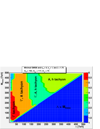
Figure 5: Regions in MMM parameter space $\Lambda$–$M_{\text{mess}}$. The lower-diagonal part is ruled out as $\Lambda>M_{\text{mess}}$. In the upper-diagonal part, from left to right, the first region (red) tachyonic $\tau^{\prime}$, and the second (orange), third (cyan), fourth (green) do not have consistent radiative electroweak symmetry breaking as indicated by the tachyonic Higgses.

Choosing the masses for the fourth generation to be given by 3 and $\tan\beta=1.75$, we have computed the supersymmetric spectrum at the weak scale. We vary $10\text{ TeV}\leq\Lambda,M_{\text{mess}}\leq 500\text{ TeV}$. The results are characterised by various regions in the parameter space as shown in 5. The blue region in the lower diagonal part is ruled out, because the messenger scale $M_{\text{mess}}$ is smaller than $\Lambda$. The greater part of the parameter space does not have radiative electroweak symmetry breaking as indicated by the tachyonic Higgs scalars (orange, cyan, and green regions) and is thus ruled out. There is, however, a small red region where electroweak symmetry breaking is possible, but the $\widetilde{\tau}^{\prime}$ is a tachyon.

Higgses [GeV]				Gauginos [GeV]				Squarks & Sleptons [GeV]
	$h^{0}$	46.2			$\widetilde{\chi}^{0}_{1}$	64.3		$\widetilde{u}_{L}$	758.1	$\widetilde{t}_{1}$	766.1	$\widetilde{t}_{1}^{\prime}$	722.6
	$A^{0}$	507.6			$\widetilde{\chi}^{0}_{2}$	127.0		$\widetilde{u}_{R}$	735.5	$\widetilde{t}_{2}$	639.3	$\widetilde{t}_{2}^{\prime}$	583.8
	$H^{0}$	532.2			$\widetilde{\chi}^{0}_{3}$	640.6		$\widetilde{d}_{L}$	761.1	$\widetilde{b}_{1}$	725.1	$\widetilde{b}_{1}^{\prime}$	733.4
	$H^{\pm}$	516.1			$\widetilde{\chi}^{0}_{4}$	655.1		$\widetilde{d}_{R}$	733.8	$\widetilde{b}_{2}$	734.3	$\widetilde{b}_{2}^{\prime}$	525.5
					$\widetilde{\chi}^{\pm}_{1}$	126.9		$\widetilde{e}_{L}$	208.3	$\widetilde{\tau}_{1}$	208.4	$\widetilde{\tau}_{1}^{\prime}$	320.3
					$\widetilde{\chi}^{\pm}_{2}$	652.0		$\widetilde{e}_{R}$	88.1	$\widetilde{\tau}_{2}$	87.8	$\widetilde{\tau}_{2}^{\prime}$	193.4
					$\widetilde{g}$	438.4		$\widetilde{\nu}_{e}$	197.2	$\widetilde{\nu}_{\tau}$	197.2	$\widetilde{\nu}_{\tau}^{\prime}$	202.7

Table 3: Minimal GMSB spectrum with 4 generations: $n_{5}=1$ GeV, $M_{\text{mess}}=100$ TeV, $\Lambda=50$ TeV, $\tan\beta=1.75$, $\text{sgn\,}\mu$=+. $\widetilde{\tau}^{\prime}$ is tachyonic, $m_{h}=46.2$ GeV, $m_{\widetilde{G}}=1.2\times 10^{-9}$ GeV (gravitino), NLSP is neutralino.

It is interesting to study in detail the region of the tachyonic $\widetilde{\tau}^{\prime}$ , with

$$10\text{ TeV}\lesssim\Lambda\lesssim 70\text{ TeV},\quad 30\text{ TeV}\lesssim M_{X}\lesssim 300\text{ TeV}.$$

A sample spectrum of this region is given in 3 where we have chosen $\Lambda$ = 50 TeV and $M_{\text{mess}}$ = 100 TeV. Notice that the light Higgs mass does not satisfy the LEP-II constraints for this point in the parameter space.

To trace the reasons for a tachyonic $\widetilde{\tau}^{\prime}$, let us consider its mass matrix which is given by

$$m^{2}_{\widetilde{\tau}^{\prime}}=\left(\begin{array}[]{cc}m^{2}_{\sc LL}&m^{2}_{\sc LR}\\ m^{2\,*}_{\sc LR}&m^{2}_{\sc RR}\end{array}\right)={\bf O}^{T}\left(\begin{array}[]{cc}m^{2}_{\widetilde{\tau}^{\prime}_{1}}&0\\ 0&m^{2}_{\widetilde{\tau}^{\prime}_{2}}\end{array}\right){\bf O},$$ (15)

where

$$m^{2}_{\sc LL} \equiv m^{2}_{\widetilde{\tau}^{\prime}_{L}}+m_{\tau^{\prime}}^{2}-m^{2}_{Z}\cos 2\beta\left(\frac{1}{2}-\sin^{2}\theta_{W}\right)\enspace\approx\enspace m^{2}_{\widetilde{\tau}^{\prime}_{L}}$$

$$m^{2}_{\sc RR} \equiv m^{2}_{\widetilde{\tau}^{\prime}_{R}}+m_{\tau^{\prime}}^{2}-m^{2}_{Z}\cos 2\beta\sin^{2}\theta_{W}\enspace\approx\enspace m^{2}_{\widetilde{\tau}^{\prime}_{R}}$$

$$m^{2}_{\sc LR} \equiv v_{d}~{}(A^{*}_{\tau^{\prime}}-\mu~{}y_{\tau^{\prime}}\tan\beta)\enspace\approx\enspace-m_{\tau^{\prime}}\mu\tan\beta$$ (16)

where ${\bf O}$ is some mixing matrix which diagonalises the $\widetilde{\tau}^{\prime}$ mass matrix. Unless both $\widetilde{\tau}^{\prime}$ are tachyonic, the condition that there is no tachyon in the spectrum is given by:

$$m^{2}_{\widetilde{\tau}^{\prime}_{L}}m^{2}_{\widetilde{\tau}^{\prime}_{R}}-(m_{\tau^{\prime}}\,\mu\tan\beta)^{2}>0$$ (17)

In the MMM model, it is typical that $\mu$ is very large, between one TeV to tens of TeV. In our analysis, $\mu$ is determined at the weak scale by electroweak symmetry breaking conditions. With $m_{\tau^{\prime}}=75$ GeV, the second term of 17 is quite large. After the RG evolution, the soft terms for $\widetilde{\tau}_{L,R}$ take the form [54]:

$$m^{2}_{\widetilde{\tau}^{\prime}_{L}}(qZ) \approx m^{2}_{\widetilde{L}}(X)-\tilde{\alpha}_{\tau^{\prime}}(2m_{\widetilde{L}}^{2}(X)+m_{\widetilde{E}}^{2}(X))\log(X/qZ)$$

$$m^{2}_{\widetilde{\tau}^{\prime}_{R}}(qZ) \approx m^{2}_{\widetilde{E}}(X)-2\tilde{\alpha}_{\tau^{\prime}}(2m_{\widetilde{L}}^{2}(X)+m_{\widetilde{E}}^{2}(X))\log(X/qZ)$$ (18)

where $\tilde{\alpha}_{\tau^{\prime}}=y_{\tau^{\prime}}^{2}\big{/}(16\pi^{2})\approx 1.1\times 10^{-3}\times(1+\tan^{2}\beta)$,  $qZ\approx 1$ TeV is the typical supersymmetric mass scale close to the weak scale, and $X$ represents the messenger scale as before. Note that the log-factor is extremely small, $\sim~{}4.6$. Thus, the effective difference between the high scale and the weak scale sleptons is very small, $\sim(5-10)\%$. For this reason, it becomes difficult to maintain 17 positive. Thus, the MMM model is perhaps too restrictive for the case of four generations. With modified boundary conditions at the messenger scale, it might be possible that gauge mediated supersymmetry breaking could lead to a phenomenologically viable spectrum. This brings us to the new ideas of general gauge mediation (GGM).

4.2 General Gauge Mediation

In the last couple of years, there has been a paradigm shift in the way we understand gauge mediated supersymmetry breaking. Ref. [55] has introduced the framework of general gauge mediation where the starting point is that the hidden sector and the visible MSSM sector should completely decouple in the limit where the gauge couplings are set to zero. The generalisation lies in the set of formulae for the soft terms which span from models with a weakly coupled messenger sector as well as to the strongly coupled ones. The general gauge mediation can allow for different scales for the scalars and the gaugino masses, with $\Lambda_{S}$ for scalar masses and $\Lambda_{G}$ for gaugino masses. In fact, the authors of Ref. [56] argue that with this kind of parametrisation, the GMSB analysis is closer to mSUGRA where the role of $\Lambda_{G}$ is played by $m_{1/2}$ and that of $\Lambda_{S}$ is played by $m_{0}$. Such freedom in the choice of scales could lead to a relaxation of the parameter space. Finally, let us note that this framework of general gauge mediation does not have any solution to the $\mu$-problem as it is not generated through the above interactions. Typical solutions of the $\mu$-problem could decouple the Higgs sector from the sleptonic sector which might pave way for the solution to the tachyonic $\widetilde{\tau}$ problem. A more detailed exploration regarding these issues will be addressed in a forthcoming publication.

5 Summary and Outlook

In the present work, we have revisited in detail the perturbativity constraints on the fourth generation Yukawa couplings in the minimal supersymmetric standard model. We have shown that if the fourth generation masses lie close to their present upper limits (or within 25% of these limits), it is possible to have perturbativity only up to $\sim$ 1000 TeV; $\tan\beta$ is confined to be very low in these models, $\sim 3$. This makes it hard to reconcile gravity mediated supersymmetry breaking models with four generations unless one assumes additional vector-like matter. However, as demonstrated in the spectrum of the toy model of mSUGRA with four generations, the presence of a fourth generation can lead to new features like lighter gluino and squark masses which could be accessible at LHC.

With this motivation, we have studied gauge mediated supersymmetry breaking with four generations. We have explored the already highly constrained minimal messenger model with the ranges allowed and found that in most of the parameter space, radiative electroweak symmetry breaking is not possible. There is a small region where electroweak symmetry breaking is viable but $\widetilde{\tau}^{\prime}$ is tachyonic. It is difficult to accommodate a fourth generation in the highly constrained minimal messenger model. We speculate that the more general framework of general gauge mediation would be suited to get phenomenologically viable mass spectra with four generations.

The combination of supersymmetry and four generations seems to lead to interesting supersymmetric spectroscopy at the weak scale. In the present work, we have just explored possible supersymmetry breaking scenarios which can work within this framework. However, four generational MSSM would have strong implications in various other sectors like flavour physics, neutrino physics and most interestingly the Higgs physics in MSSM. These aspects as well as concrete models within gauge mediation need to be studied. Experimental consequences of the presence of the fourth generation with SUSY, in B-physics, D-physics as well as direct detection at LHC needs to be investigated.

Acknowledgements

We acknowledge useful discussions with Ben Allanach, Jörg Meyer, Sandip Pakvasa and Arun Prasath. SKV acknowledges support by DST Project No : SR/S2/HEP-0018/2007 of Govt. of India. RMG acknowledges the support of Department of Science and Technology, India, under the J.C. Bose fellowship SR/S2/JCB-64/2007.

Appendix A The Renormalisation Group Equations

For completeness, we list the 2-loop renormalisation group equations for the gauge and Yukawa couplings that we have used to generalise SOFTSUSY to the case of the MSSM with $n_{G}$ chiral generations. These RGEs can be derived from the general case [57, 58, 59] and are well-known in the literature [60, 61, 62, 16, 63, 64, 18]. Here we are following Ref. [64].

A.1 The Gauge Couplings

The running of the gauge couplings is given by

$$\frac{dg_{i}}{dt}=-\frac{1}{16\pi^{2}}\,b_{i}g_{i}^{3}+\frac{g_{i}^{3}}{(16\pi^{2})^{2}}\left[\sum_{k}b_{ik}g_{k}^{2}-{\rm Tr}\left\{C_{iu}{\bf Y}_{u}^{\dagger}{\bf Y}_{u}+C_{id}{\bf Y}_{d}^{\dagger}{\bf Y}_{d}+C_{ie}{\bf Y}_{e}^{\dagger}{\bf Y}_{e}\right\}\right],$$ (19)

where $t=\log(\mu/\mu_{0})$, $\mu$ is the renormalisation scale, $\mu_{0}$ some reference scale, and $i,k=1,2,3$ refer to the gauge groups $\text{U}(1)_{Y}$, $\text{SU}(2)_{L}$ and $\text{SU}(3)_{c}$. At 1-loop, the $b_{i}$ are given by

$$b_{1}=-\frac{3}{5}-2n_{G},\qquad b_{2}=5-2n_{G},\qquad b_{3}=9-2n_{G}.$$ (20)

The fourth generation comes in complete GUT multiplets, and thus most predictions from grand unification are unchanged. In fact, the only modification at 1-loop is that $\alpha_{\textsc{gut}}$ increases. At 2-loop, the Yukawa couplings enter the RGEs, and the coefficients are given by

$$\left(b\right)_{ik}=n_{G}\left(\begin{array}[]{ccc}\frac{38}{15}&\frac{6}{5}&\frac{88}{15}\\ \frac{2}{5}&14&8\\ \frac{11}{15}&3&\frac{68}{3}\\ \end{array}\right)+\left(\begin{array}[]{ccc}\frac{9}{25}&\frac{9}{5}&0\\ \frac{3}{5}&\text{-}17&0\\ 0&0&\text{-}54\\ \end{array}\right),\qquad\left(C\right)_{if}=\left(\begin{array}[]{ccc}\frac{26}{5}&\frac{14}{5}&\frac{18}{5}\\ 6&6&2\\ 4&4&0\\ \end{array}\right)$$ (21)

where $i,k=1,2,3$ as before, and $f=u,d,e$.

A.2 The Yukawa Couplings

The running of the Yukawa couplings is given by

$$\frac{d}{dt}{\bf Y}_{u,d,e}={\bf Y}_{u,d,e}\left(\frac{1}{16\pi^{2}}\boldsymbol{\beta}_{u,d,e}^{(1)}+\frac{1}{(16\pi^{2})^{2}}\boldsymbol{\beta}_{u,d,e}^{(2)}\right).$$ (22)

At 1-loop, the $\beta$-function coefficients are:

$$\boldsymbol{\beta}_{u}^{(1)} =3{\bf Y}_{u}^{\dagger}{\bf Y}_{u}+{\bf Y}_{d}^{\dagger}{\bf Y}_{d}+3{\rm Tr}\left\{{\bf Y}_{u}^{\dagger}{\bf Y}_{u}\right\}-\left(\frac{13}{15}g_{1}^{2}+3g_{2}^{2}+\frac{16}{3}g_{3}^{2}\right)$$ (23)

$$\boldsymbol{\beta}_{d}^{(1)} =3{\bf Y}_{d}^{\dagger}{\bf Y}_{d}+{\bf Y}_{u}^{\dagger}{\bf Y}_{u}+{\rm Tr}\left\{3{\bf Y}_{d}^{\dagger}{\bf Y}_{d}+{\bf Y}_{e}^{\dagger}{\bf Y}_{e}\right\}-\left(\frac{7}{15}g_{1}^{2}+3g_{2}^{2}+\frac{16}{3}g_{3}^{2}\right)$$ (24)

$$\boldsymbol{\beta}_{e}^{(1)} =3{\bf Y}_{e}^{\dagger}{\bf Y}_{e}+{\rm Tr}\left\{3{\bf Y}_{d}^{\dagger}{\bf Y}_{d}+{\bf Y}_{e}^{\dagger}{\bf Y}_{e}\right\}-\left(\frac{9}{5}g_{1}^{2}+3g_{2}^{2}\right)$$ (25)

Note that the number of generations enters only through the dimensionality of the Yukawa matrices. At 2-loop, $n_{G}$ is explicitly present, and the $\beta$-function coefficients are:

$$\boldsymbol{\beta}_{u}^{(2)} = -4({\bf Y}_{u}^{\dagger}{\bf Y}_{u})^{2}-2({\bf Y}_{d}^{\dagger}{\bf Y}_{d})^{2}-2{\bf Y}_{d}^{\dagger}{\bf Y}_{d}{\bf Y}_{u}^{\dagger}{\bf Y}_{u}-9{\rm Tr}\left\{{\bf Y}_{u}^{\dagger}{\bf Y}_{u}\right\}{\bf Y}_{u}^{\dagger}{\bf Y}_{u}$$ (26)

$$\mbox{}-{\rm Tr}\left\{3{\bf Y}_{d}^{\dagger}{\bf Y}_{d}+{\bf Y}_{e}^{\dagger}{\bf Y}_{e}\right\}{\bf Y}_{d}^{\dagger}{\bf Y}_{d}-3{\rm Tr}\left\{3({\bf Y}_{u}^{\dagger}{\bf Y}_{u})^{2}+{\bf Y}_{d}^{\dagger}{\bf Y}_{d}{\bf Y}_{u}^{\dagger}{\bf Y}_{u}\right\}$$

$$\mbox{}+(\frac{2}{5}g_{1}^{2}+6g_{2}^{2}){\bf Y}_{u}^{\dagger}{\bf Y}_{u}+(\frac{2}{5}g_{1}^{2}){\bf Y}_{d}^{\dagger}{\bf Y}_{d}+(\frac{4}{5}g_{1}^{2}+16g_{3}^{2}){\rm Tr}\left\{{\bf Y}_{u}^{\dagger}{\bf Y}_{u}\right\}$$

$$\mbox{}+(\frac{26}{15}n_{G}+\frac{403}{450})g_{1}^{4}+(6n_{G}-\frac{21}{2})g_{2}^{4}+(\frac{32}{3}n_{G}-\frac{304}{9})g_{3}^{4}$$

$$\mbox{}+g_{1}^{2}g_{2}^{2}+\frac{136}{15}g_{1}^{2}g_{3}^{2}+8g_{2}^{2}g_{3}^{2}$$

$$\boldsymbol{\beta}_{d}^{(2)} = -4({\bf Y}_{d}^{\dagger}{\bf Y}_{d})^{2}-2({\bf Y}_{u}^{\dagger}{\bf Y}_{u})^{2}-2{\bf Y}_{u}^{\dagger}{\bf Y}_{u}{\bf Y}_{d}^{\dagger}{\bf Y}_{d}-3{\rm Tr}\left\{{\bf Y}_{u}^{\dagger}{\bf Y}_{u}\right\}{\bf Y}_{u}^{\dagger}{\bf Y}_{u}$$ (27)

$$\mbox{}-3{\rm Tr}\left\{3{\bf Y}_{d}^{\dagger}{\bf Y}_{d}+{\bf Y}_{e}^{\dagger}{\bf Y}_{e}\right\}{\bf Y}_{d}^{\dagger}{\bf Y}_{d}-3{\rm Tr}\left\{3({\bf Y}_{d}^{\dagger}{\bf Y}_{d})^{2}+({\bf Y}_{e}^{\dagger}{\bf Y}_{e})^{2}+{\bf Y}_{d}^{\dagger}{\bf Y}_{d}{\bf Y}_{u}^{\dagger}{\bf Y}_{u}\right\}$$

$$\mbox{}+(\frac{4}{5}g_{1}^{2}){\bf Y}_{u}^{\dagger}{\bf Y}_{u}+(\frac{4}{5}g_{1}^{2}+6g_{2}^{2}){\bf Y}_{d}^{\dagger}{\bf Y}_{d}+(-\frac{2}{5}g_{1}^{2}+16g_{3}^{2}){\rm Tr}\left\{{\bf Y}_{d}^{\dagger}{\bf Y}_{d}\right\}+(\frac{6}{5}g_{1}^{2}){\rm Tr}\left\{{\bf Y}_{e}^{\dagger}{\bf Y}_{e}\right\}$$

$$\mbox{}+(\frac{14}{15}n_{G}+\frac{7}{18})g_{1}^{4}+(6n_{G}-\frac{21}{2})g_{2}^{4}+(\frac{32}{3}n_{G}-\frac{304}{9})g_{3}^{4}+g_{1}^{2}g_{2}^{2}+\frac{8}{9}g_{1}^{2}g_{3}^{2}+8g_{2}^{2}g_{3}^{2}$$

$$\boldsymbol{\beta}_{e}^{(2)} = -4({\bf Y}_{e}^{\dagger}{\bf Y}_{e})^{2}-3{\rm Tr}\left\{3{\bf Y}_{d}^{\dagger}{\bf Y}_{d}+{\bf Y}_{e}^{\dagger}{\bf Y}_{e}\right\}{\bf Y}_{e}^{\dagger}{\bf Y}_{e}-3{\rm Tr}\left\{3({\bf Y}_{d}^{\dagger}{\bf Y}_{d})^{2}+({\bf Y}_{e}^{\dagger}{\bf Y}_{e})^{2}\right.$$ (28)

$$\mbox{}\left.+{\bf Y}_{d}^{\dagger}{\bf Y}_{d}{\bf Y}_{u}^{\dagger}{\bf Y}_{u}\right\}+(6g_{2}^{2}){\bf Y}_{e}^{\dagger}{\bf Y}_{e}+(\frac{6}{5}g_{1}^{2}){\rm Tr}\left\{{\bf Y}_{e}^{\dagger}{\bf Y}_{e}\right\}+(-\frac{2}{5}g_{1}^{2}+16g_{3}^{2}){\rm Tr}\left\{{\bf Y}_{d}^{\dagger}{\bf Y}_{d}\right\}$$

$$\mbox{}+(\frac{18}{5}n_{G}+\frac{27}{10})g_{1}^{4}+(6n_{G}-\frac{21}{2})g_{2}^{4}+\frac{9}{5}g_{1}^{2}g_{2}^{2}$$

A.3 Approximate Upper Bounds

An approximate upper bound on the fourth generation $t^{\prime}$ can be obtained in the limit where $m_{t^{\prime}}$ dominates over all the other masses, $m_{t^{\prime}}\gg\{m_{t},~{}m_{b^{\prime}},~{}m_{\tau^{\prime}}\}$ purely from perturbative requirements. To see this, let us rewrite 22 in terms of the dominant Yukawa couplings:

$$\beta_{h_{t^{\prime}}} = h_{t^{\prime}}\left(6h_{t^{\prime}}^{2}+h_{b^{\prime}}^{2}+3h_{t}^{2}-{16\over 3}g_{3}^{2}-3g_{2}^{2}-{13\over 15}g_{1}^{2}\right)$$

$$\beta_{h_{b^{\prime}}} = h_{b^{\prime}}\left(6h_{b^{\prime}}^{2}+h_{t^{\prime}}^{2}+h_{\tau^{\prime}}^{2}-{16\over 3}g_{3}^{2}-3g_{2}^{2}-{7\over 15}g_{1}^{2}\right)$$

$$\beta_{h_{\tau^{\prime}}} = h_{\tau^{\prime}}\left(3h_{b^{\prime}}^{2}+4h_{\tau^{\prime}}^{2}-3g_{2}^{2}-{9\over 5}g_{1}^{2}\right)$$

$$\beta_{h_{t}} = h_{t}\left(3h_{t^{\prime}}^{2}+6h_{t}^{2}-{16\over 3}g_{3}^{2}-3g_{2}^{2}-{13\over 15}g_{1}^{2}\right)$$ (29)

These equations are non-linear and coupled and obviously, should be solved numerically. However an analytical estimate can be obtained in the above mentioned limit $m_{t^{\prime}}\gg\{m_{t},~{}m_{b^{\prime}},~{}m_{\tau^{\prime}}\}$. In this limit the solution for $h_{t^{\prime}}$ can be written as [65] :

$$k_{t^{\prime}}(z)={E(z)k_{t^{\prime}}(0)\over(1+6k_{t^{\prime}}(0)F(z))},$$ (30)

where $z=2\log(M_{X}/M_{Z})$ with $M_{X}$ denoting the high scale and $M_{Z}$, the weak scale. $k_{t^{\prime}}=h_{t^{\prime}}^{2}/(4\pi)$ and

$$E(z) = \left(1+\tilde{b}_{1}{\alpha_{1}(0)\over 4\pi}z\right)^{{13\over 9\tilde{b}_{1}}}\left(1+\tilde{b}_{2}{\alpha_{2}(0)\over 4\pi}z\right)^{{3\over\tilde{b}_{2}}}\left(1+\tilde{b}_{3}{\alpha_{3}(0)\over 4\pi}z\right)^{{16\over 3\tilde{b}_{3}}}$$

$$F(z) = \int_{0}^{z}E(z^{\prime})dz^{\prime}$$ (31)

$k_{t^{\prime}}(0)$ is the value of the $t^{\prime}$ Yukawa (squared) at the high scale, $M_{X}$. These are the same expressions one obtains for the top quark Yukawa coupling within three generations. In four generations, the only difference is the $\beta$-functions of the gauge couplings. In 31, $\tilde{b}_{i}=-b_{i}$, and from 20, $\tilde{b}_{3}=-1$, $\tilde{b}_{2}=3$, $\tilde{b}_{1}=43/3$. If the Yukawa coupling becomes very large, from 30, we can derive an upper bound on the (square) of the Yukawa of the top-prime in the limit $k_{t^{\prime}}(0)\to\infty$:

$$k_{t^{\prime}}(z)\sim{E(z)\over 6~{}F(z)}$$ (32)

In 4 we present the upper limits on the $m_{t^{\prime}}$ in this approximate limit using 32. We see that the present limit on the $m_{t^{\prime}}$ readily rules out perturbativity up to the Planck scale or even the GUT scale. If we demand perturbativity beyond 1-100 TeV, $m_{t^{\prime}}$ is forced to be close to its experimental present lower bound or below. Beyond $10^{6}$ GeV the present limit already rules out perturbative a Yukawa coupling for the $t^{\prime}$. As we have seen in the main text, demanding perturbativity of the $b^{\prime}$ and $\tau^{\prime}$ Yukawa couplings would put further stringent constraints on the scale $M_{X}$.

$M_{X}$ (GeV)	$10^{18}$	$10^{16}$	$10^{11}$	$10^{6}$	$10^{3}$
$m_{t^{\prime}}$ (GeV)	211.3	212.8	222.2	264.2	437.7

Table 4: The approximate upper limits on $m_{t^{\prime}}$ in the limit where $m_{t^{\prime}}$ dominates over all the masses, for various high scales, $M_{X}$.

Appendix B INDISOFT

In this appendix, we summarise the most important features of the software tool that we have developed to calculate soft spectra in the MSSM with four generations. More details will be presented in a separate publication.

INDISOFT is based on SOFTSUSY 3.0.9. [50]. We have preserved the original C++ class structure and extended the functionality of the individual classes that handle the calculations. It is beyond the scope of the present appendix to describe SOFTSUSY in detail, and we refer for that to its manual [50].

The fermion masses and gauge coupling constants are stored in the class QedQcd which we have extended to comprise also the fourth generation fermion masses. The light fermion masses and the couplings that are entered at different scales (depending on where they are experimentally known) are then run to $M_{Z}$ using the class RGE that implements the renormalisation group running for every class that derives from it, in this case for QedQcd. For the heavy fermions, we have generalised the functions that calculate the pole mass from the running one and vice versa. From now on we will assume that we are working in a framework (like mSUGRA or gauge mediation) where the soft masses are obtained from boundary conditions set at a higher scale. The class MssmSusy is derived from RGE and contains the supersymmetric parameters of the theory; the Yukawa matrices have been promoted to $4\times 4$ matrices to include the fourth generation. The $\beta$-functions of MssmSusy have been generalised to the case of four generations (see Appendix A). The class SoftParsMssm is derived from MssmSusy and contains the soft supersymmetry-breaking terms of the MSSM; the soft mass matrices and the trilinear couplings have been generalised; the supersymmetric parameters and their RGE evolution are inherited from MssmSusy; the $\beta$-functions of SoftParsMssm for the soft terms have been generalised. The class MssmSoftsusy derives from SoftParsMssm and organises the actual calculation of the spectrum. QedQcd is used to initialise/guess the susy parameters at the scale $m_{t}$ which are then run by RGE to the high scale $M_{X}$ where the boundary conditions on the soft terms are imposed. Note that for the gauge and Yukawa couplings, we use 2-loop RGEs (see Appendix A), and 1-loop RGEs for the rest. MssmSoftsusy is then run back to $M_{\textsc{susy}}{}$ ($=M_{Z}$ for the first iteration), where the electroweak symmetry breaking conditions are checked and the physical spectrum is calculated (at tree-level for the first iteration, and later at 1-loop). The class sPhysical that calculates the physical masses and stores the results has been generalised to handle four generations. The class drBarPars that derives from sPhysical and manages the $\overline{\text{DR}}$ parameters for the calculation has been generalised. The tadpoles, 1-loop radiative corrections to the Higgses, squarks, sleptons, and the threshold corrections to the gauge couplings have been generalised to include contributions from the fourth generation fermions. The aforementioned steps are iterated until satisfactory convergence is achieved.

As a result of our work, we found some minor typos and bugs in SOFTSUSY that have been fixed in subsequent versions. We have rewritten the linear algebra classes from scratch, replacing the pointer constructions used to represent vectors/matrices and the algorithms operating on them by the Standard Template Library (STL) containers and algorithms. In addition to the presently available mSUGRA and minimal GMSB boundary conditions, we have implemented a model of general gauge mediation along the lines of Ref. [56]. We have linked ROOT [66] to our programs to generate plots both interactively and in batch mode. In future, we plan to extend INDISOFT by right-handed neutrinos. Due to space limitations, we must refrain from discussing all the changes we have made.

References

- [1] DØ Collaboration, V. M. Abazov et al., “Observation of Single Top-Quark Production,” Phys. Rev. Lett. 103 (2009) 092001, 0903.0850.
- [2] CDF Collaboration, T. Aaltonen et al., “First Observation of Electroweak Single Top Quark Production,” Phys. Rev. Lett. 103 (2009) 092002, 0903.0885.
- [3] J. Alwall et al., “Is V(tb) = 1?,” Eur. Phys. J. C49 (2007) 791–801, hep-ph/0607115.
- [4] G. D. Kribs, T. Plehn, M. Spannowsky, and T. M. P. Tait, “Four generations and Higgs physics,” Phys. Rev. D76 (2007) 075016, 0706.3718.
- [5] M. Bobrowski, A. Lenz, J. Riedl, and J. Rohrwild, “How much space is left for a new family of fermions?,” Phys. Rev. D79 (2009) 113006, 0902.4883.
- [6] M. S. Chanowitz, “Bounding CKM Mixing with a Fourth Family,” Phys. Rev. D79 (2009) 113008, 0904.3570.
- [7] B. Holdom et al., “Four Statements about the Fourth Generation,” 0904.4698.
- [8] V. A. Novikov, A. N. Rozanov, and M. I. Vysotsky, “Once more on extra quark-lepton generations and precision measurements,” 0904.4570.
- [9] P. Q. Hung and M. Sher, “Experimental constraints on fourth generation quark masses,” Phys. Rev. D77 (2008) 037302, 0711.4353.
- [10] P. H. Frampton, P. Q. Hung, and M. Sher, “Quarks and leptons beyond the third generation,” Phys. Rept. 330 (2000) 263, hep-ph/9903387.
- [11] H. B. Nielsen, A. V. Novikov, V. A. Novikov, and M. I. Vysotsky, “Higgs potential bounds on extra quark - lepton generations,” Phys. Lett. B374 (1996) 127–130, hep-ph/9511340.
- [12] Y. F. Pirogov and O. V. Zenin, “Two-loop renormalization group restrictions on the standard model and the fourth chiral family,” Eur. Phys. J. C10 (1999) 629–638, hep-ph/9808396.
- [13] H. Goldberg, “The fourth generation and N=1 Supergravity,” Phys. Lett. B165 (1985) 292.
- [14] K. Enqvist, D. V. Nanopoulos, and F. Zwirner, “The Fourth Generation in Supergravity,” Phys. Lett. B164 (1985) 321.
- [15] R. L. Arnowitt and P. Nath, “Fourth Generation and Nucleon Decay in Supersymmetric Theories,” Phys. Rev. D36 (1987) 3423–3428.
- [16] M. Drees, K. Enqvist, and D. V. Nanopoulos, “No Future for the Fourth Generation?,” Nucl. Phys. B294 (1987) 1.
- [17] J. F. Gunion, D. W. McKay, and H. Pois, “Gauge coupling unification and the minimal SUSY model: a Fourth generation below the top?,” Phys. Lett. B334 (1994) 339–347, hep-ph/9406249.
- [18] J. F. Gunion, D. W. McKay, and H. Pois, “A Minimal four family supergravity model,” Phys. Rev. D53 (1996) 1616–1647, hep-ph/9507323.
- [19] J. E. Dubicki and C. D. Froggatt, “Supersymmetric grand unification with a fourth generation?,” Phys. Lett. B567 (2003) 46–52, hep-ph/0305007.
- [20] Z. Murdock, S. Nandi, and Z. Tavartkiladze, “Perturbativity and a Fourth Generation in the MSSM,” Phys. Lett. B668 (2008) 303–307, 0806.2064.
- [21] P. Q. Hung, “Minimal SU(5) resuscitated by long-lived quarks and leptons,” Phys. Rev. Lett. 80 (1998) 3000–3003, hep-ph/9712338.
- [22] W.-S. Hou, “CP Violation and Baryogenesis from New Heavy Quarks,” Chin. J. Phys. 47 (2009) 134, 0803.1234.
- [23] R. Fok and G. D. Kribs, “Four Generations, the Electroweak Phase Transition, and Supersymmetry,” Phys. Rev. D78 (2008) 075023, 0803.4207.
- [24] Y. Kikukawa, M. Kohda, and J. Yasuda, “The strongly coupled fourth family and a first-order electroweak phase transition (I) quark sector,” 0901.1962.
- [25] E. De Pree, G. Marshall, and M. Sher, “The Fourth Generation t-prime in Extensions of the Standard Model,” Phys. Rev. D80 (2009) 037301, 0906.4500.
- [26] G. Burdman and L. Da Rold, “Electroweak Symmetry Breaking from a Holographic Fourth Generation,” JHEP 12 (2007) 086, 0710.0623.
- [27] A. Borstnik Bracic, M. Breskvar, D. Lukman, and N. S. Mankoc Borstnik, “A new understanding of fermion masses from the unified theory of spins and charges,” hep-ph/0606224.
- [28] H. Stremnitzer and J. C. Pati, “New Crucial Tests of Compositeness of the Third and a Possible Fourth Family in e+ e- Colliders,” Phys. Lett. B196 (1987) 240.
- [29] M. T. Frandsen, I. Masina, and F. Sannino, “Fourth Lepton Family is Natural in Technicolor,” 0905.1331.
- [30] O. Antipin, M. Heikinheimo, and K. Tuominen, “Natural fourth generation of leptons,” 0905.0622.
- [31] B. Holdom, “Heavy Quarks and Electroweak Symmetry Breaking,” Phys. Rev. Lett. 57 (1986) 2496.
- [32] C. T. Hill, M. A. Luty, and E. A. Paschos, “Electroweak symmetry breaking by fourth generation condensates and the neutrino spectrum,” Phys. Rev. D43 (1991) 3011–3025.
- [33] S. F. King, “Is Electroweak Symmetry Broken by a Fourth Family of Quarks?,” Phys. Lett. B234 (1990) 108–112.
- [34] G. Kramer and I. Montvay, “Radiative Quark Mass Generation and a Fourth Quark Family,” Zeit. Phys. C11 (1981) 159.
- [35] A. L. Kagan, “Radiative Quark Mass and Mixing Hierarchies from Supersymmetric Models with a Fourth Mirror Family,” Phys. Rev. D40 (1989) 173.
- [36] M. Sher and Y. Yuan, “Cosmological bounds on the lifetime of a fourth generation charged lepton,” Phys. Lett. B285 (1992) 336–342.
- [37] H. Fritzsch, “Light neutrinos, nonuniversality of the leptonic weak interaction and a fourth massive generation,” Phys. Lett. B289 (1992) 92–96.
- [38] C. T. Hill and E. A. Paschos, “A Naturally Heavy Fourth Generation Neutrino,” Phys. Lett. B241 (1990) 96.
- [39] K. S. Babu, S. Nandi, and Z. Tavartkiladze, “New Mechanism for Neutrino Mass Generation and Triply Charged Higgs Bosons at the LHC,” Phys. Rev. D80 (2009) 071702, 0905.2710.
- [40] M. Drees, K. Enqvist, and D. V. Nanopoulos, “The Fourth Generation in Superstring Models,” Phys. Lett. B189 (1987) 321.
- [41] Particle Data Group Collaboration, C. Amsler et al., “Review of particle physics,” Phys. Lett. B667 (2008) 1.
- [42] CDF Collaboration, T. Aaltonen et al., “Search for Heavy Top-like Quarks Using Lepton Plus Jets Events in 1.96-TeV Collisions,” Phys. Rev. Lett. 100 (2008) 161803, 0801.3877.
- [43] DØ Collaboration, S. Abachi et al., “Top quark search with the DØ 1992 - 1993 data sample,” Phys. Rev. D52 (1995) 4877–4919.
- [44] CDF Collaboration, T. Aaltonen et al., “Search for New Particles Leading to jets Final States in Collisions at = 1.96- TeV,” Phys. Rev. D76 (2007) 072006, 0706.3264.
- [45] CDF Collaboration, D. E. Acosta et al., “Search for long-lived charged massive particles in collisions at TeV,” Phys. Rev. Lett. 90 (2003) 131801, hep-ex/0211064.
- [46] L3 Collaboration, P. Achard et al., “Search for heavy neutral and charged leptons in annihilation at LEP,” Phys. Lett. B517 (2001) 75–85, hep-ex/0107015.
- [47] DELPHI Collaboration, P. Abreu et al., “Searches for heavy neutrinos from Z decays,” Phys. Lett. B274 (1992) 230–238.
- [48] R. Rattazzi and U. Sarid, “The Unified minimal supersymmetric model with large Yukawa couplings,” Phys. Rev. D53 (1996) 1553–1585, hep-ph/9505428.
- [49] B. Ananthanarayan, G. Lazarides, and Q. Shafi, “Top mass prediction from supersymmetric guts,” Phys. Rev. D44 (1991) 1613–1615.
- [50] B. C. Allanach, “SOFTSUSY: A C++ program for calculating supersymmetric spectra,” Comput. Phys. Commun. 143 (2002) 305–331, hep-ph/0104145.
- [51] S. Litsey and M. Sher, “Higgs Masses in the Four Generation MSSM,” Phys. Rev. D80 (2009) 057701, 0908.0502.
- [52] G. F. Giudice and R. Rattazzi, “Theories with gauge-mediated supersymmetry breaking,” Phys. Rept. 322 (1999) 419–499, hep-ph/9801271.
- [53] M. Drees, R. Godbole, and P. Roy, “Theory and phenomenology of sparticles: An account of four-dimensional N=1 supersymmetry in high energy physics,”. Hackensack, USA: World Scientific (2004) 555 p.
- [54] F. Borzumati, “On the minimal messenger model,” hep-ph/9702307.
- [55] P. Meade, N. Seiberg, and D. Shih, “General Gauge Mediation,” Prog. Theor. Phys. Suppl. 177 (2009) 143–158, 0801.3278.
- [56] S. Abel, M. J. Dolan, J. Jaeckel, and V. V. Khoze, “Phenomenology of Pure General Gauge Mediation,” 0910.2674.
- [57] M. E. Machacek and M. T. Vaughn, “Two Loop Renormalization Group Equations in a General Quantum Field Theory. 1. Wave Function Renormalization,” Nucl. Phys. B222 (1983) 83.
- [58] M. E. Machacek and M. T. Vaughn, “Two Loop Renormalization Group Equations in a General Quantum Field Theory. 2. Yukawa Couplings,” Nucl. Phys. B236 (1984) 221.
- [59] N. K. Falck, “Renormalization Group Equations for Softly Broken Supersymmetry: The Most General Case,” Z. Phys. C30 (1986) 247.
- [60] J. E. Bjorkman and D. R. T. Jones, “The Unification Mass, and in Nonminimal Supersymmetric SU(5),” Nucl. Phys. B259 (1985) 533.
- [61] J. Bagger, S. Dimopoulos, and E. Masso, “Renormalization Group Constraints in Supersymmetric Theories,” Phys. Rev. Lett. 55 (1985) 920.
- [62] M. Cvetic and C. R. Preitschopf, “Heavy Families and N=1 Supergravity Within the Standard Model,” Nucl. Phys. B272 (1986) 490.
- [63] M. Tanimoto, Y. Suetake, and K. Senba, “Fritzsch Mass Matrix with the Fourth Generation and the Renormalization Group Equations,” Phys. Rev. D36 (1987) 2119.
- [64] D. J. Castano, E. J. Piard, and P. Ramond, “Renormalization group study of the Standard Model and its extensions. 2. The Minimal supersymmetric Standard Model,” Phys. Rev. D49 (1994) 4882–4901, hep-ph/9308335.
- [65] L. E. Ibanez and C. Lopez, “N=1 Supergravity, the Weak Scale and the Low-Energy Particle Spectrum,” Nucl. Phys. B233 (1984) 511.
- [66] R. Brun and F. Rademakers, “ROOT: An object oriented data analysis framework,” Nucl. Instrum. Meth. A389 (1997) 81–86.