Statistics and geometry of cosmic voids

Abstract:

We introduce new statistical methods for the study of cosmic voids, focusing on the statistics of largest size voids. We distinguish three different types of distributions of voids, namely, Poisson-like, lognormal-like and Pareto-like distributions. The last two distributions are connected with two types of fractal geometry of the matter distribution. Scaling voids with Pareto distribution appear in fractal distributions with box-counting dimension smaller than three (its maximum value), whereas the lognormal void distribution corresponds to multifractals with box-counting dimension equal to three. Moreover, voids of the former type persist in the continuum limit, namely, as the number density of observable objects grows, giving rise to lacunar fractals, whereas voids of the latter type disappear in the continuum limit, giving rise to non-lacunar (multi)fractals. We propose both lacunar and non-lacunar multifractal models of the cosmic web structure of the Universe. A non-lacunar multifractal model is supported by current galaxy surveys as well as cosmological $N$-body simulations. This model suggests, in particular, that small dark matter halos and, arguably, faint galaxies are present in cosmic voids.

1 Introduction

The large scale structure of the Universe is formed by matter clusters, filaments and sheets, and also cosmic voids. Cosmic voids are the counterpart of matter structures. They have arisen in observations of the galaxy distribution and have gradually become the subject of deep theoretical investigations. Early studies of cosmic voids were conditioned by the small number of galaxies surveyed then. For example, Otto et al. [1] studied the significance of cosmic voids, to distinguish them from fluctuations of a homogeneous galaxy distribution. They developed probabilistic methods for the study of voids but they actually concluded that cosmic voids were not really significant. Betancort-Rijo [2] improved and generalized their methods and reached the opposite conclusion. The rôle of voids as a basic ingredient of the large scale structure is now well established [3, 4, 5].

However, the definition of what constitutes a void is still imprecise. Originally, voids were described as large regions devoid of galaxies and found by visual inspection. As this is hardly satisfactory, an objective way of identifying voids has been long sought. To identify a void in a point distribution, one needs to decide if it is to be empty or it can have a few points inside and one further needs to determine its shape. The simplest option, preferred by Otto et al. [1] and Einasto et al. [3], is to define voids as empty spheres. Kauffmann and Fairall [4] also demand that voids be empty but devise a void-finder that allows more general shapes, with the intention to find approximately ellipsoidal voids. ElAd and Piran [5] devise an even more elaborate method: they assume that there is a set of highly clustered “wall galaxies” and implement a procedure to select them before the void-finding phase, which joins empty spheres with a “thinness” limitation. Therefore, the found voids are not empty of galaxies and can have fairly complex shapes.

The preceding definitions of voids ignore that galaxy voids can contain dark matter. Although there is no substantial observational knowledge of the geometry of voids in the dark matter distribution, we have information from cosmological $N$-body simulations. For example, Gottlöber et al [6] re-simulate voids with higher resolution and find structures inside them, in a self-similar pattern. This suggests that the definition of voids as empty regions of simple shape is not appropriate in this case. Shandarin, Sheth & Sahni [7] and Sheth & van de Weygaert [8] define voids as under-dense regions of a continuous density field, such that they are complementary to matter clusters. With this definition, voids contain matter and have very complex shapes. Shandarin et al. [7] and Sheth & van de Weygaert [8] extend methods that have been used successfully for the study of clusters to the study of voids. In fact, under-densities and over-densities are symmetrical in a Gaussian random field.

Colberg et al [9] have presented an overview of various void definitions and have made a comparison of the results of applying the corresponding void finding algorithms to the same data set.

The choice of a simple definition of voids, in particular, their definition as empty spheres, is convenient for statistical studies of galaxy voids. On the other hand, the geometrical aspects of dark-matter voids that arise in cosmological simulations are difficult to relate to the statistics of spherical voids. The definition of dark-matter voids as under-densities in a Gaussian field is appealing but difficult to connect with any notion of empty voids. In fact, a Gaussian density field is a valid description only in the linear regime of gravitational clustering, but empty or nearly empty voids are very nonlinear structures. Therefore, a suitable description of the geometry of voids demands the use of nonlinear models of the cosmic structure. We focus on fractal models, for they are well founded and provide a useful description of voids.

Fractal models of the large-scale structure of the Universe were introduced by Mandelbrot [10] and have been well studied [11, 12, 13], but they are still controversial [12]. The major controversy concerns the transition to homogeneity. Mandelbrot [10], inspired by old hierarchical models of the Universe without transition to homogeneity, has indeed suggested that there might not be an outer cutoff to the fractal scaling range. Assuming that there is a scale of homogeneity, scale invariance is nevertheless justified on smaller scales by observational and theoretical arguments. The observation of a power-law two-point correlation function of galaxies in a range of scales [14] was one of Mandelbrot’s motivations and is still a strong argument. Furthermore, there are evidences of scaling in higher order correlation functions [12].

Theoretical arguments for scale invariance are based on the absence of scales in the gravitational dynamics of collision-less cold dark matter (CDM). This nonlinear dynamics indeed gives rise to a hierarchical formation of structures on every scale up to the homogeneity scale, which grows with time. Thus, we can reasonably expect that the resulting structure consists in a (multi)fractal attractor of the nonlinear dynamics. Structure formation in CDM models is studied with $N$-body simulations, which support a multifractal model in a range of scales [15, 16, 17, 18, 19]. This range is restricted by the intrinsic limitations of these $N$-body simulations (even of state-of-the-art simulations). The limitations are much less stringent for one-dimensional cosmological dynamics, which is simulated by Miller et al [20], finding multifractal structure in a very long range of scales. One last but not least argument for scale invariance is that the cosmic web produced by the adhesion model [21] is found to have multifractal features [22, 23].

Mandelbrot [10] has also introduced the notion of fractal holes (“tremas”) and considered its application to the galaxy distribution. In particular, he has introduced the notion of fractal lacunarity as a measure of the size of voids in fractals of equal dimension. For any given dimension, one can construct a set of different fractals with progressively decreasing lacunarity, leading to the possibility of a non-lacunar fractal. Mandelbrot [10] indeed shows an example of non-lacunar fractal, the Besicovitch fractal, which in modern terminology belongs to the class of multinomial multifractals. Mandelbrot [10] is actually concerned about the low perceived lacunarity of the galaxy distribution and how to reconcile it with the power-law galaxy correlation function. In our present study of cosmic voids, a non-lacunar fractal indeed appears as the most suitable model.

At any rate, most fractal models of the galaxy distribution proposed so far are lacunar and imply a self-similar distribution of cosmic voids. The self-similarity of voids has been considered by Einasto et al [3] as a probe for scale invariance in the large scale structure. Following the ideas of Mandelbrot [10], we have established that the rank-ordering of fractal void sizes fulfills Zipf’s power law and tried to confirm it with data from galaxy surveys [24]. Thus far, the scaling of galaxy voids remains moot: our analysis does not show any evidence [24], but analyses of recent surveys are more favourable [25, 26, 27]. However, it is questionable that these scalings hold in a sufficiently long range.

In a multifractal geometry, it is natural to define voids as the locations of mass depletions [18]. This notion of voids is more general than the notion of voids as empty holes and, actually, allows us to define voids in non-lacunar fractals. We study here the geometry of multifractal voids, which is connected with the geometry of under-densities in a Gaussian field but is actually more complicated. From the multifractal geometry of dark matter voids, we can derive the geometry of galaxy voids with a model of galaxy biasing. We consider a simple biasing model, inspired by the “peak theory” of Gaussian fields [28], but we substitute Gaussian peaks by multifractal mass concentrations, in accord with the multifractal model of dark matter halos that we have proposed in Refs. [29, 18]. Our model provides a new perspective on Peebles’ “void phenomenon” [30], regarding the emptiness of voids.

We begin with the probabilistic analysis of voids in point distributions. We calculate the probability of spherical voids and the size of the largest void in a Poisson distribution (Sect. 2). We proceed to the general probability of voids in correlated point distributions (Sect. 3) but we obtain less complete results. We introduce the hierarchical Poisson model and the lognormal model as typical distributions and we connect them with fractal distributions. To measure the statistics of spherical voids in samples, we devise an efficient void-finder in Sect. 4. In Sect. 5, we adopt a geometrical viewpoint centered on fractal distributions and, in particular, cut-out sets, which we consider as cosmic web models. We generalize this construction to multifractals and thence we proceed to a general study of multifractal voids, which leads us to differentiate two types of voids according to their geometry (Sect. 6). This general study of multifractal voids is combined in Sect.7 with the results of Sect. 3 to characterize the voids in cosmological simulations and galaxy samples In particular, we deduce some properties of galaxy voids in Sect. 7.2, assuming a multifractal model of galaxy biasing. We summarize our results and present our conclusions in Sect. 8. Finally, we include three appendices to deal with technical points.

2 Poissonian analysis of cosmic voids

2.1 The probability of voids

Let us recall the formulation of cosmic voids by Otto et al. [1], based on the results of Politzer & Preskill [31]. They first quantify the fluctuations in a sample of randomly distributed points (a homogeneous Poisson field). If the density of points is $n$, then the probability of having $k$ points in a region of volume $V$ is given by the familiar Poisson distribution with parameter $N=nV$:

$${P}_{k}[V]=\frac{N^{k}}{k!}\,e^{-N}.$$

The condition $k\ll N$ means that the given region is devoid of points. However, the calculation of the probability of having a void of given size and shape at any place is difficult. Politzer & Preskill’s analysis [31] yields the following formula for the probability per unit total volume that there is some region of volume $V$ and given shape that contains $k$ points:

$$\mathbb{P}_{k}[V]=c_{s}\,\frac{(nV)^{3}}{V}\,{P}_{k}[V]\,,$$

where $c_{s}$ is a coefficient that depends on the shape. To prove this formula, they simulate the action of a void-finding algorithm. Thus, they calculate $c_{s}$ for spherical voids.

The simplest shape of a void is certainly the spherical shape. Let us call $\mathbb{P}_{k}[V]$ the probability density of having a volume $V$ spherical void containing $k$ points. A sphere containing $k$ points is defined by four (non-coplanar) points on its boundary, because the sphere can always be enlarged so as to touch four points. We call it a $k$-void, understanding that $k\ll nV$. $\mathbb{P}_{k}[V]$ can be estimated from a sample of the Poisson distribution by counting the total number of $k$-voids and, then, dividing the number of them that have volume between $V$ and $V+dV$ by their total number. To calculate the number of $k$-voids and $\mathbb{P}_{k}[V]$ analytically, we can employ the following method.

Since the points are uncorrelated, the probability distribution for each point is constant and independent of the other points. The number density of point quadruplets is simply the product

$$\frac{n^{4}}{4!}\,d^{3}x_{1}\,d^{3}x_{2}\,d^{3}x_{3}\,d^{3}x_{4}\,,$$

where the denominator takes into account that the points are unordered. Its integral over the total volume is the total number of quadruplets $N_{\rm t}(N_{\rm t}-1)(N_{\rm t}-2)(N_{\rm t}-3)/4!\approx N_{\rm t}^{4}/4!$, being $N_{\rm t}$ the total number of points. We can calculate the number density of $k$-voids as the product of the total density of quadruplets and the probability ${P}_{k}[V]$, where $V$ is the volume of the sphere that corresponds to a given quadruplet. Therefore, the only problem is to express the four-point volume element in terms of a set of variables that includes the volume of that sphere. If we denote the position of the center of the sphere (the quadruplet’s circumcenter) by $x_{\rm c}$, then the required number density is

$$\frac{n^{4}}{4!}\,{P}_{k}[V]\,d^{3}x_{1}\,d^{3}x_{2}\,d^{3}x_{3}\,d^{3}x_{4}=$$

$$\frac{n^{4}}{4!}\,d^{3}x_{\rm c}\,{P}_{k}[V]\,V^{2}\,dV\,f({\mbox{\boldmath{$\theta$}}}_{1},{\mbox{\boldmath{$\theta$}}}_{2},{\mbox{\boldmath{$\theta$}}}_{3},{\mbox{\boldmath{$\theta$}}}_{4})\,d^{2}{\mbox{\boldmath{$\theta$}}}_{1}\,d^{2}{\mbox{\boldmath{$\theta$}}}_{2}\,d^{2}{\mbox{\boldmath{$\theta$}}}_{3}\,d^{2}{\mbox{\boldmath{$\theta$}}}_{4},$$ (1)

where $\{{\mbox{\boldmath{$\theta$}}}_{i}\}_{i=1}^{4}$ are the four sets of two angular coordinates over the sphere, and $f$ is a function of these angular coordinates. This expression follows from translation invariance and dilation covariance only. The function $f$ is calculated explicitly in Appendix A.

To calculate the number of $k$-voids of volume $V$, we integrate the right-hand side of Eq. (1) over all variables except $V$. If we further integrate over $V$, we obtain the total number of $k$-voids. The integral of $n\,d^{3}x_{\rm c}$ can be factored out, making the number of $k$-voids proportional to the total number of points $N_{t}$. The integral of $f$ over the angular coordinates yields the factor $4!\,12\pi^{2}/35$ (see Appendix A). Therefore, the number of $k$-voids with volume between $V$ and $V+dV$, per point of the sample, is

$$\frac{12\,\pi^{2}}{35}\,{P}_{k}[V]\,n^{3}\,V^{2}\,dV\,,$$

and the total number of $k$-voids per point is

$$\frac{12\,\pi^{2}}{35}\int_{0}^{\infty}\frac{N^{k}}{k!}\,e^{-N}N^{2}\,dN=\frac{12\,\pi^{2}}{35}\,(k+2)(k+1)\,.$$

In particular, the number of voids (0-voids) per point is $24\pi^{2}/35=6.76773$. It is interesting to compare this number with the numbers that correspond to regular lattices. For example, we can consider a body centered cubic lattice, which has six void quadruplets (tetrahedra) per point [32]. There are regular lattices with more voids per point, so it is not surprising that the value in the random case is larger than six.

To obtain the probability of $k$-voids $\mathbb{P}_{k}[V]$, we divide the number of $k$-voids of volume $V$ by the total number of $k$-voids:

$$\mathbb{P}_{k}[V]=\frac{1}{(k+2)(k+1)}\,\frac{(nV)^{3}}{V}\,{P}_{k}[V]\,.$$ (2)

Note that the name $k$-void makes sense only if $V\gg k/n$, but 0-voids are voids for any $V$. ${P}_{0}[V]$ approaches unity in the limit $V\rightarrow 0$, but $\mathbb{P}_{0}[V]$ is small in this limit, due to the boundary factor (corresponding to the four points defining the void). In other words, the probability that a randomly chosen small ball be empty is large, but the probability that it have four points on its boundary and thus constitute a void is small. In fact, the most probable void size (the mode) is $V=2/n$. We can calculate other statistical quantities, for example, the mean void size ${\overline{V}}=3/n$.

We can generalize the above method to other void shapes, e.g., ellipsoidal voids, and indeed to any shape defined by a finite number of points. The number of $k$-voids has an expression generalizing Eq. (1), where the exponent of $V$ is the number of points minus two; e.g, an ellipsoid is defined by nine boundary points. The number of $k$-voids is always proportional to the number of sample points $N_{\rm t}$. However, the function $f$ of angular coordinates can be very complicated, and we may not be able to integrate it and, thus, obtain the proportionality constant. Nonetheless, $\mathbb{P}_{k}[V]$ is a power of $V$ with the given exponent, and the normalization constant is easy to obtain.

Otto et al. [1] applied their results to determining the significance of some large voids that had been found at the time and concluded that those voids were not significant, namely, that they did not rule out a Poisson distribution. The conclusion that large voids are not significant was contradicted by Betancort-Rijo [2] and does not hold anymore, regarding recent galaxy surveys. One recent survey is studied in Sect. 7.2. In the next section, we study in detail the statistics of large voids in Poisson distributions.

2.2 Extreme values: the largest and smallest voids

Following Otto et al. [1], we consider the size of the largest void in a given sample as the most important statistic. Indeed, the largest voids are the ones to be first perceived. In general, the statistics of extreme values is useful for data that are naturally rank ordered. The largest value is the most important one. The smallest value and, hence, the total range can also be useful statistics, for example, in a list of voids obtained with a void-finder. The theory of extreme values is a classic subject in statistics. A brief introduction to it is given by Sornette [33].

The rank order is related to the cumulative distribution $\mathbb{P}_{>}[V]=\int_{V}^{\infty}\mathbb{P}_{0}[v]\,dv$, which we often employ in this work. In an $M$-sample of this distribution, namely, a sample of $M$ void sizes, the rank of one of them is the number of values larger than or equal to it, that is, the order in the sorted list $V_{1}\geq\cdots\geq V_{M}$. If we have several $M$-samples available, we can obtain the distribution of sizes for each rank and its average. If $M=1$, we can adopt as average value the median $V_{\rm med}$, such that $\mathbb{P}_{>}[V_{\rm med}]=1/2$. In the general case of $M$-samples, suitable average values are given by $\mathbb{P}_{>}[V_{m}]=m/(M+1)$, where $m$ denotes the rank. Thus, the largest value $V_{1}$ fulfills $\mathbb{P}_{>}[V_{1}]=1/(M+1)$ and the smallest one fulfills $\mathbb{P}_{>}[V_{M}]=M/(M+1)$.

For spherical voids in the Poisson distribution, we can calculate $\mathbb{P}_{>}[V]$ from Eq. (2) (with $k=0$):

$$\mathbb{P}_{>}[V]=\left(1+nV+\frac{(nV)^{2}}{2}\right)e^{-nV}\,.$$ (3)

The probable sizes of the largest and smallest voids can be obtained by solving the corresponding equations. Although these equations involve the total number of voids $M$ rather than the total number of points $N_{\rm t}$, we know that $M=6.77\,N_{\rm t}$. Of course, we assume that this number is large. Thus, the equation for the largest void is

$$\mathbb{P}_{>}[V_{1}]\approx\frac{(nV_{1})^{2}}{2}\,e^{-nV_{1}}=\frac{1}{M}.$$ (4)

Letting $N_{1}=nV_{1}$ denote the number of points that correspond to the largest void volume, we are to solve the equation

$$N_{1}=\ln\frac{M}{2}+2\ln N_{1}\,.$$

It can be solved iteratively, starting with $N_{1}=1$. We obtain the asymptotic expansion

$$N_{1}=\ln\frac{M}{2}+2\ln\ln\frac{M}{2}+\cdots$$ (5)

For a sample with $N_{\rm t}=10\hskip 1.0pt000$ points, $N_{1}\simeq\ln 33\hskip 1.0pt839+2\ln\ln 33\hskip 1.0pt839\simeq 15.$

It is easy to generalize these results to non-spherical voids: in Eq. (3), the corresponding terms of higher degree are to be added to the polynomial in its right-hand side. Consequently, the coefficient of the sub-leading term in Eq. (5) is larger. Besides, the coefficient of proportionality between $M$ and $N_{\rm t}$ grows as well, but this has a smaller effect. Although the shape of voids is, in principle, a sub-leading effect, the polynomial in the right-hand side of Eq. (3) tends to $e^{nV}$ as the number of points that define the shape of voids goes to infinity and, therefore, $\mathbb{P}_{>}[V]$ tends to one. In other words, the volume of the voids grows with no bound when we remove any constraint on their shape, as is natural. In Sect. 4, we mention constraints that are suitable for void-finding algorithms.

The equation for the smallest void is

$$\mathbb{P}_{>}[V_{M}]\approx\left(1+nV_{M}\right)e^{-nV_{M}}=\frac{M}{M+1}\approx 1-\frac{1}{M}\,,$$ (6)

with solution

$$N_{M}=\frac{1}{\sqrt{M}}\,.$$ (7)

For spherical voids in $N_{\rm t}=10\hskip 1.0pt000$ points, there are about $67\hskip 1.0pt677$ voids and the smallest void is such that $N_{67\hskip 1.0pt677}=0.0038$.

We can estimate the probable volume of the largest void in another way, by using $P_{0}[V]$, which is the probability that a given region of volume $V$ be empty. Given a sample with total volume $V_{\rm t}$, let us tile it with $V_{\rm t}/V$ regions of volume $V$, for example, applying a cubic mesh to it. The expected number of empty regions is $P_{0}[V](V_{\rm t}/V)$. Therefore, if only one of them is to be empty, then we have the equation $P_{0}[V](V_{\rm t}/V)=1$ or

$$e^{-N_{1}}=\frac{N_{1}}{N_{\rm t}}.$$

This equation can also be solved iteratively, yielding

$$N_{1}=\ln N_{\rm t}-\ln\ln N_{\rm t}+\cdots$$

For $N_{\rm t}=10\hskip 1.0pt000$ points, now $N_{1}\simeq 7$. Since $P_{0}[V]$ is the probability that a given region of volume $V$ be empty, it represents a random trial region that is unlikely to be empty even if it intersects the largest void of the same volume (as pointed out by Otto et al. [1]). Therefore, this method underestimates the size of the largest void. Nevertheless, the leading logarithmic term is the same as the leading term in Eq. (5), obtained from $\mathbb{P}_{>}[V]$.

By just taking the leading term $\ln N_{\rm t}$, we can deduce that the relative size of the largest void, namely, the fraction of the sample’s volume that it occupies, vanishes as $N_{\rm t}\rightarrow\infty$. In other words, voids disappear in the continuum limit $n\rightarrow\infty$ of a Poisson distribution, as is natural.

3 The probability of voids in correlated point distributions

It is possible to extend the preceding methods to correlated distributions of particles. Otto et al. [1] already derived one formula for the probability of voids in correlated point distributions, in terms of an expansion in powers of the density $n$. Betancort-Rijo [2] employed instead a non-perturbative method based on the expression of $P_{0}[V]$ in terms of the probability of density fluctuations. We take inspiration from both approaches to generalize the preceding calculations. Ultimately, we intend to find the behavior of the probability of voids in distributions with strong correlations, namely, in distributions with strong mass concentrations. In particular, we study fractal distributions.

3.1 The general probability of voids

The probability of spherical voids in the general case is studied by Otto et al. using expansions in powers of the density $n$ [1]. The function ${P}_{0}[V]$ (void probability function) was previously expressed by White [34] as

$${P}_{0}[V]=\exp\left[\sum_{k=1}^{\infty}\frac{(-nV)^{k}}{k!}\,{\bar{\xi}}_{k}\right],$$ (8)

where ${\bar{\xi}}_{1}=1$, and, for $k\geq 2$, ${\bar{\xi}}_{k}$ is the average in $V$ of the correlation function ${\xi}_{k}$:

$${\bar{\xi}}_{k}=\frac{1}{V^{k}}\int_{V}d^{3}x_{1}\cdots d^{3}x_{k}\,\xi_{k}(x_{1},\ldots,x_{k}).$$

${P}_{0}[V]$ is analogous to the grand-canonical partition function in statistical mechanics (with velocities integrated over) and the expansion in terms of the ${\bar{\xi}}_{k}$ (the cumulants) is analogous to the cluster expansion. This connection was noticed by Otto et al. [1] and is considered further by Mekjian [35]. We assume that the cumulants ${\bar{\xi}}_{k}$ ($k\geq 2$) always vanish in the limit $V\rightarrow\infty$ and that they vanish the more rapidly the larger $k$ is. Thus, the first correction to the Poisson formula is given by a non-vanishing ${\bar{\xi}}_{2}$ (a Gaussian field). Of course, Eq. (8) is only valid insofar as the expansion converges (see Sect. 3.2).

White [34] noticed that ${P}_{0}[V]$ can also be expressed, using the local particle density $\rho$, as the integral over $\rho$ of the product of the probability of $\rho$ and the probability of a void volume $V$ given that the density is $\rho$. The latter probability is given by the Poisson formula. Therefore,

$${P}_{0}[V]=\int\limits_{0}^{\infty}P(\rho)\,\exp\left[-\rho V\right]d\rho\,.$$ (9)

The exponential inside the integral can be expanded in powers of $\rho V$ and, assuming that the integration and the sum can be interchanged, ${P}_{0}[V]$ becomes an expansion in terms of moments:

$${P}_{0}[V]=\sum_{k=0}^{\infty}\frac{(-nV)^{k}}{k!}\,{\bar{\mu}}_{k}\,,$$ (10)

where the moments are defined by

$${\bar{\mu}}_{k}=\int\limits_{0}^{\infty}\left(\frac{\rho}{n}\right)^{k}P(\rho)\,d\rho=\frac{1}{(nV)^{k}}\int_{V}d^{3}x_{1}\cdots d^{3}x_{k}\,\langle\rho(x_{1})\cdots\rho(x_{k})\rangle,$$

with $n=\langle\rho\rangle$ (note that ${\bar{\mu}}_{1}\equiv 1$). Of course, the moment expansion in Eq. (10) is equivalent to the cumulant expansion in Eq. (8). However, the integral expression (9) is more general and is always valid (see Sect. 3.2) .

If we remove the density fluctuations by making $P(\rho)=\delta(\rho-n)$, we recover the Poisson formula, that is, the first term in the expansion (8). If we account for small fluctuations by taking a Gaussian $P(\rho)$ [2], we further obtain the second term in the expansion (8). We must also consider a variant of the Poisson distribution, such that the total space is divided in two regions, one being empty and another having the Poisson distribution. This second region is meant to be formed by matter clusters (of uniform density). If $n_{\mathrm{c}}$ denotes the density inside the clusters, we have that

$$P(\rho)=\left(1-\frac{n}{n_{\mathrm{c}}}\right)\delta(\rho)+\frac{n}{n_{\mathrm{c}}}\,\delta(\rho-n_{\mathrm{c}}).$$

The two constants before the delta functions are deduced from the normalization of $P(\rho)$ and the condition $\langle\rho\rangle=n$. The void probability function given by Eq. (9) is

$${P}_{0}[V]=1-\frac{n}{n_{\mathrm{c}}}\left(1-e^{-n_{\mathrm{c}}V}\right)=1+\frac{n}{n_{\mathrm{c}}}\sum_{k=1}^{\infty}\frac{(-n_{\mathrm{c}}V)^{k}}{k!}\,.$$ (11)

Comparing it with Eq. (10), we deduce that ${{\bar{\mu}}_{2}}=n_{\mathrm{c}}/n$ and that the moments fulfill the hierarchical relation ${\bar{\mu}}_{k}={{\bar{\mu}}_{2}}^{k-1}$. This hierarchical model is especially interesting when $n_{\mathrm{c}}\gg n$, namely, when the volume occupied by the matter clusters is a small fraction of the total volume. Then, it coincides with Fry’s hierarchical Poisson model [36], with

$${P}_{0}[V]=\exp\left[-\frac{1-e^{-nV{\bar{\xi}}_{2}}}{{\bar{\xi}}_{2}}\right]$$ (12)

(note that then ${\bar{\xi}}_{2}={\bar{\mu}}_{2}-1\gg 1$). Hierarchical models are related to fractal models [37, 11], which we study in detail in Sect. 3.4.

The moments always satisfy the inequality ${\bar{\mu}}_{k}\geq{{\bar{\mu}}_{2}}^{k-1}$, among other inequalities [38]. As we have seen, the lowest allowed value of ${\bar{\mu}}_{k}$ occurs in distributions that are uniform inside their support. In spite of this uniformity, there are strong density fluctuations in the total volume when $n_{\mathrm{c}}\gg n$, since the support is sparse. We now consider the lognormal model [39], which can have strong density fluctuations inside its support, such that ${\bar{\mu}}_{k}\gg{{\bar{\mu}}_{2}}^{k-1}$. This model is also related to fractal models.

For the lognormal model,

$${P}_{0}[V] = \frac{1}{\sigma\sqrt{2\pi}}\int\limits_{0}^{\infty}\exp\left[-\frac{(\ln\rho-\mu)^{2}}{2\sigma^{2}}-\rho V\right]\frac{d\rho}{\rho}$$ (13)

$$= \frac{1}{\sigma\sqrt{2\pi}}\int\limits_{0}^{\infty}\exp\left[-\frac{(\ln r+\sigma^{2}/2)^{2}}{2\sigma^{2}}-r\,nV\right]\frac{dr}{r}\,,$$

where $\mu=\ln n-\sigma^{2}/2$ (with $n=\langle\rho\rangle$) and we have made the change of variable $r=\rho/n$ to obtain the second integral. We can restrict the support of this distribution as well, with the consequent addition of a constant to ${P}_{0}[V]$ and substitution of $n$ by $n_{\mathrm{c}}$. But we understand that the support is the total volume, for the moment. The constant $\sigma$ in Eq. (13) actually depends on $V$, and $P(\rho)$ becomes Gaussian and eventually uniform as $V$ grows and $\sigma\rightarrow 0$. However, if we take $\sigma\simeq 1$, then the probability that a relatively large volume be empty, namely, that $V\gg n^{-1}$, is much larger that the corresponding Poisson value. For example, with $\sigma=1$ and $nV=10$, Eq. (13) yields ${P}_{0}[V]=0.0539$, whereas $\exp(-10)=0.0000454$.

The lognormal moments are easily evaluated, yielding ${\bar{\mu}}_{k}=\exp\left[k(k-1)\sigma^{2}/2\right]$. In the limit $\sigma\rightarrow 0$, ${\bar{\mu}}_{k}$ tends to one and ${\bar{\xi}}_{k}$ vanishes (if $k\geq 2$). Moreover, the cumulants actually vanish the more rapidly the larger $k$ is. In the opposite limit, when $\sigma$ is large, the moments grow exponentially and, furthermore, ${\bar{\mu}}_{k}\gg{{\bar{\mu}}_{2}}^{k-1}$.

3.1.1 Calculation of the distribution of voids

To calculate the number of spherical voids in a correlated point distribution, the expression for a quadruplet of uncorrelated points in the left-hand side of Eq. (1) must be replaced by

$$\frac{n^{4}}{4!}\,d^{3}x_{1}\cdots d^{3}x_{4}\left[{\zeta_{1}}(x_{1}){\zeta_{1}}(x_{2}){\zeta_{1}}(x_{3}){\zeta_{1}}(x_{4})+\right.$$

$$\left.{\zeta_{2}}(x_{1},x_{2}){\zeta_{1}}(x_{3}){\zeta_{1}}(x_{4})+\cdots+{\zeta_{1}}(x_{1}){\zeta_{1}}(x_{2}){\zeta_{2}}(x_{3},x_{4})+\right.$$

$${\zeta_{2}}(x_{1},x_{2}){\zeta_{2}}(x_{3},x_{4})+\cdots+{\zeta_{2}}(x_{1},x_{4}){\zeta_{2}}(x_{2},x_{3})+$$

$${\zeta_{3}}(x_{1},x_{2},x_{3}){\zeta_{1}}(x_{4})+\cdots+{\zeta_{1}}(x_{1}){\zeta_{3}}(x_{2},x_{3},x_{4})+$$

$$\left.{\zeta_{4}}(x_{1},\ldots,x_{4})\right]{P}_{0}[V]\,,$$ (14)

where the ${\zeta}(\cdot)$ are correlation functions conditioned by the presence of the void (using White’s general definitions [34]). These correlation functions can be expanded in powers of $n$ and written in terms of ordinary correlation functions:

$${\zeta_{1}}(x) = 1+\sum_{k=1}^{\infty}\frac{(-n)^{k}}{k!}\int_{V}d^{3}y_{1}\cdots d^{3}y_{k}\,\xi_{k+1}(x,y_{1},\ldots,y_{k}),$$

$${\zeta_{2}}(x_{1},x_{2}) = {\xi}_{2}(x_{1},x_{2})+$$

$$\sum_{k=1}^{\infty}\frac{(-n)^{k}}{k!}\int_{V}d^{3}y_{1}\cdots d^{3}y_{k}\,\xi_{k+2}(x_{1},x_{2},y_{1},\ldots,y_{k}),$$

etc. In particular, ${\zeta_{1}}(x)$ is independent of $x$, due to translation invariance, and $n\,{\zeta_{1}}$ can be interpreted as a conditional density. From expression (14), we can proceed like in the Poisson case, namely, we can express the four-point volume element in terms of the sphere’s volume and angular variables, factor out $n\,d^{3}x_{\rm c}$, and then integrate over the angular coordinates. Unfortunately, this integration cannot be explicitly worked out in the general case, because the ${\zeta}(\cdot)$ depend on the angular coordinates.

Naturally, an expression for the number of non-spherical voids, e.g., ellipsoidal voids, can also be written; but it is even less tractable than the expression for spherical voids. On the other hand, we could consider $k$-voids instead of empty voids. Needless to say, the extra $k$ points also make the expressions less tractable.

In one dimension, the geometry is much simpler. In general, only the two-point function is involved in the expression corresponding to (14), there are no angular coordinates, and there is one void interval per point. Therefore,

$$\mathbb{P}_{0}[L]=\frac{n}{2}\,[\zeta_{1}^{2}+\zeta_{2}(L)]\,{P}_{0}[L].$$ (15)

Of course, this one-dimensional formula is not directly applicable to three-dimensional cosmic voids, but it is applicable to void intervals in pencil-beam surveys, as measured by Einasto et al [3], for example.

3.2 Scope of the perturbative expansions in the density

The expansions in powers of the density used in the preceding section require that the density be small, in a sense that we need to make precise. The simplest expansion to study is the cumulant expansion of $P_{0}[V]$ given by Eq. (8). The successive terms of this series are expected to be of small magnitude and eventually decreasing. In particular, the second term of the series is smaller than the first (Poisson) term if $N=nV<{\bar{\xi}}_{2}^{-1}$. We can interpret this condition in terms of the number variance in the volume $V$, namely,

$$\frac{\langle\delta\!N^{2}\rangle}{N^{2}}=\frac{1}{N}+{\bar{\xi}}_{2}\,.$$

When $N<{\bar{\xi}}_{2}^{-1}$ the Poisson fluctuations dominate over the fluctuations due to correlations, and vice versa. However, the cumulant expansion (8) can converge in spite of having initial terms that increase. For example, the expansion of $P_{0}$ for Fry’s hierarchical Poisson model in Eq. (12) converges for any value of $N{\bar{\xi}}_{2}$, although the initial terms increase in magnitude when $N{\bar{\xi}}_{2}>1$, until the $k$th term is such that $k\approx N{\bar{\xi}}_{2}$. Thus, when $N{\bar{\xi}}_{2}\gg 1$, it is necessary to sum a large number of terms, some of which are large (in absolute value), to obtain a negligible sum, for $e^{-N{\bar{\xi}}_{2}}\rightarrow 0$ as ${N{\bar{\xi}}_{2}}\rightarrow\infty$. This makes the series unsuitable for numerical computations.

The cumulant expansion of the lognormal model has worse behavior. Indeed, the integral formula (13) shows that $P_{0}[V]$ is not analytic at $V=0$ [39]. In consequence, the moment expansion (10) must diverge. This also follows from the expression ${\bar{\mu}}_{k}=\exp\left[k(k-1)\sigma^{2}/2\right]$. $\ln P_{0}[V]$ is also not analytic at $V=0$ and the cumulant expansion diverges as well. Actually, the moment and cumulant expansions are asymptotic as $N\rightarrow 0$. They also are alternating series. An alternating asymptotic series converges while its terms are of decreasing magnitude, and it must be terminated at the term with the least magnitude (which should be included with half its value). Therefore, a small value of $N{\bar{\xi}}_{2}$ is mandatory. We can relate the bad behavior of these density expansions in the case of strong clustering ($\sigma\gg 1$) to the strong growth of moments, such that ${\bar{\mu}}_{k}\gg{{\bar{\mu}}_{2}}^{k-1}$. This strong growth of moments is typical of certain distributions, in particular, multifractals.

For the lognormal void probability function at large $\sigma$, the asymptotic expansion of the integral in Eq. (13) worked out in Appendix B yields

$$P_{0}[V]=1-\frac{\sqrt{2N}}{\sigma}\,e^{-\sigma^{2}/8}\left[1+{\mathop{\rm O}\nolimits(\sigma^{-2})}\right].$$ (16)

This expression provides a reasonable approximation already for moderately large $\sigma$. For $\sigma=3$, the approximation is quite good in a relevant range of $N$. When $N=1$, the value computed directly with Eq. (13) is $P_{0}[V]=0.885346$ and the one computed with Eq. (16) is $P_{0}[V]=0.846957$. In contrast, the condition $N<{\bar{\xi}}_{2}^{-1}\simeq\exp(-\sigma^{2})=0.00012$ is far too restrictive.

The non-analyticity of the lognormal $P_{0}[V]$ at $V=0$ is due to the slow decay of its probability function $P(\rho)$ in the high density limit. In general, mass distributions that are singular on small scales possess probability functions with fat tails in the high density limit. Nevertheless, the probability function $P(\rho)$ can have moments of any order, like the lognormal distribution. Then, the series expansions of $P_{0}[V]$ or ${\zeta}(\cdot)$ are well defined, but they are asymptotic rather than convergent. Distributions with moments of any order but with fat tails such that moment and cumulant expansions diverge can be called lognormal like. In these distributions, the full set of moments or cumulants does not determine a unique function $P(\rho)$. To do this, one needs to add moments of non-integer order and even moments of negative order. In particular, the description of multifractals requires all the $q$-moments, with $q$ any real number [11, 40]

3.3 The largest void in a correlated distribution

In absence of the probability function $\mathbb{P}_{0}[V]$, we do not have detailed knowledge of the distribution of void sizes, but we can always find a lower estimate of the largest void size by using ${P}_{0}[V]$ as in Sect. 2.2: a lower estimate of the largest void size is given by the solution of the equation $P_{0}[V](V_{\rm t}/V)=1$. For example, we consider the hierarchical Poisson model, with $P_{0}[V]$ given by Eq. (11), and the lognormal $P_{0}[V]$ in Eq. (13). For the largest void, $N=nV\gg 1$, in general. Thus, we must focus on this limit, which we can interpret, alternately, as the limit of large volumes or as the continuum limit.

In the hierarchical Poisson model, we can take the continuum limit $n\rightarrow\infty$ while preserving the distribution of clusters, just by keeping ${{\bar{\mu}}_{2}}=n_{\mathrm{c}}/n$ constant. Thus, the voids inside clusters vanish while the voids between clusters are unaffected. In that limit, Eq. (11) becomes

$${P}_{0}[V]=1-\frac{n}{n_{\mathrm{c}}}=1-\frac{1}{{\bar{\mu}}_{2}}\,.$$ (17)

This quantity is close to one when the clustering is strong, namely, when ${{\bar{\mu}}_{2}}\gg 1$. Then, the fraction of empty space is large, even in the continuum limit of the distribution, and naturally we can find large voids. The largest void size is determined by the distribution of clusters, which is assumed to be a Poisson distribution.

Regarding the lognormal model, we need the asymptotic form of the integral in Eq. (13) for large $N=nV$ that is worked out in Appendix B. Keeping only the first term, we have

$$\ln P_{0}\approx-\frac{(\ln N)^{2}}{2\,\sigma^{2}}\,.$$ (18)

In this case, $\lim_{N\rightarrow\infty}P_{0}=0$, like in the Poisson distribution. Naturally, the lognormal $P_{0}[V]$ has a decrease with $V$ that is slower than the exponential decrease of the Poisson distribution. For the largest void, we have the equation:

$$-\frac{(\ln N)^{2}}{2\,\sigma^{2}}=\ln\frac{N}{N_{\rm t}}\,.$$

Its solution is simply

$$\ln N\approx\sigma\sqrt{2\ln N_{t}}\,.$$ (19)

Compared to the leading asymptotic term in the Poisson case, namely, $N=\ln N_{\rm t}$, we notice that the size of the largest void is greatly enhanced. For example, taking $N_{\rm t}=10\hskip 1.0pt000$ points and $\sigma=1$, now $N\simeq 73$. Nevertheless, the relative size $V/V_{\rm t}$ of the largest void goes to zero as $N_{\rm t}=nV_{\rm t}\rightarrow\infty$, like in the Poisson case.

A remark is in order here: $\sigma$ is not really a constant, but decreases with $V$, as we comment after Eq. (13). This fact can be taken into account to derive an equation for the size of the largest voids more accurate than Eq. (19) if we know the law $\sigma(V)$. The scaling model that we study in Sect. 3.4 provides us with a simple form of that law. At any rate, Eq. (19) is sound if $\sigma$ is of the order of unity at the scale $V$ of the largest void.

In general, the largest value in a random sample from a distribution is determined by the tail of the distribution. If the sample is very large, the distribution of the largest value must approach one of three distributions, named extreme value distributions [33]. Only two extreme value distributions are relevant in our context: the Gumbel distribution and the Fréchet-Pareto distribution (the third distribution is for bounded variables). The domain of attraction of the Gumbel distribution consists of the probability density functions with a tail falling faster than a power law. It contains the Poisson distribution of voids and also lognormal-like void probability functions. The domain of attraction of the Fréchet-Pareto distribution consists of the probability density functions with a power law tail. The Fréchet-Pareto distribution assigns considerable probability to large values and is such that the largest value is of the same order of magnitude as the sum of the remaining values, even as the number of values tends to infinity. We have found an example of this behavior in Fry’s hierarchical Poisson model. Voids of this type are typical of fractal distributions, which we study next.

3.4 Voids in scaling distributions

We have seen that the analytical description of voids is difficult when the density of points is large or the correlations are strong, namely, when $N{\bar{\xi}}_{2}>1$. Of course, the analytical treatment of strongly correlated distributions, with ${\bar{\xi}}_{2}\gg 1$, is difficult in general. Some progress can be made with the use of tractable specific models which, arguably, have general features. For example, we have mentioned that the Gumbel or Fréchet-Pareto distributions are limit distributions of the largest void, featuring a limited or unlimited size of it, respectively. As specific models, we have chosen the hierarchical Poisson model and the lognormal model, connected with the Fréchet-Pareto and Gumbel distributions, respectively. Our two specific models are also connected with fractal distributions, which have special interest.

We can introduce self-similar fractals as a generalization of the hierarchical Poisson model. This hierarchical model has only two levels in the hierarchy, namely, clusters and particles; but we can imagine that every particle is also a cluster at the adequate level of resolution, thus building a hierarchy with many levels, even an infinite number. An infinite self-similar cluster hierarchy constitutes a fractal. More formally, a fractal is a continuous distribution (with mean density $n\rightarrow\infty$) such that it has strong correlations with scaling properties; namely, the correlation functions ${\xi}_{k}$ as well as their integrals ${\bar{\xi}}_{k}$ are power laws. In particular, the two-point correlation is ${\xi}_{2}(r)=(r_{0}/r)^{\gamma}$, where $r_{0}$ is the homogeneity scale, and the relative mass variance in a cell of volume $V$ is ${\bar{\xi}}_{2}=(V_{0}/V)^{\gamma/3}$, where $V_{0}$ is a homogeneity volume (of the order of magnitude of $r_{0}^{3}$).

We must distinguish monofractals, whose scaling properties are characterized by just the exponent $\gamma$ or the dimension $D=3-\gamma$, from multifractals, which have a spectrum of dimensions. Fractal distributions can have voids in spite of being continuous and statistically homogeneous, unlike other types of distributions. For example, the Poisson distribution or lognormal-like distributions do not have voids in the continuum limit. On the other hand, when the density $n$ is finite, the fractal regime holds while $nV{\bar{\xi}}_{2}>1$, namely, for volumes $V$ such that $n\,V_{0}^{\gamma/3}\,V^{D/3}>1$.

Since a fractal distribution is scale invariant, it is reasonable to assume that the distribution of voids in a fractal is also scale invariant. Before considering the scaling of voids in three dimensions, let us consider one-dimensional fractals, in which the geometrical problems regarding the shape of voids are absent.

In one dimension, a probabilistic formulation of the scaling of voids is provided by the application of the Lévy stable distributions [10]. Their stability means that the sum of a number of independent identical variables keeps the same distribution, after rescaling. A Lévy distribution becomes a power law for sufficiently large values of its variable and, furthermore, it is an attractor of distributions with the same power-law behaviour (generalizing the central limit theorem). Therefore, a distribution such that the interval between successive points has probability $\mathbb{P}_{0}[L]\sim L^{-D-1},$ for $0<D<1$ and large $L$, converges in the continuum limit to a Lévy flight (a generalized random walk), in which $\mathbb{P}_{0}[L]\propto L^{-D-1},$ for any $L$, and the mass in an interval of length $l$ is distributed as $l^{D}$. This power-law form of $\mathbb{P}_{0}[L]$ is not integrable at $L=0$ and must be understood as a conditional probability: the probability of a void of length $L$ given that $L$ is longer than an arbitrary length $\lambda$ is the Pareto distribution $\mathbb{P}_{0}[L|L>\lambda]=D\lambda^{D}/L^{D+1}$ (see Ref. [10] and Appendix C).

Thus, the construction of a Lévy flight directly defines $\mathbb{P}_{0}[L]$, without resort to expression (15) for one-dimensional voids. In particular, the void probability function $P_{0}[L]$ tends to one and becomes irrelevant for the probability of voids. In fact, $P_{0}[L]\rightarrow 1$ as a consequence of the strong correlations between the points in a Lévy flight: a given interval is likely to contain no points, because the probability of finding one point is only non-negligible when conditioned on being close to another point. Mandelbrot [10] shows that the conditional probability of having some mass in an interval of length $l$ inside an interval of length $L$ that is known to have mass is $P[M(l)>0|M(L)>0]=(l/L)^{1-D}$. Hence, $P_{0}[L]$ is not exactly one due to the existence of the homogeneity scale $r_{0}$, and we can write

$$P_{0}[L]=1-P[M(L)>0\,|M(r_{0})>0]=1-(L/r_{0})^{1-D},$$

which tends to one as $L/r_{0}\rightarrow 0$. Remarkably, this holds independently of the value of the density $n$, even as $n\rightarrow\infty$.

Both properties, namely, $\mathbb{P}_{0}[L]\propto L^{-D-1}$ and $P_{0}[L]\rightarrow 1$ for $L\ll r_{0}$, can be generalized to other one-dimensional fractals (with voids that are not independent) and also to fractals in higher dimensions. Actually, higher-dimensional Lévy flights are not useful to model the scaling of voids, because in them an empty interval between two points does not define a void. Therefore, it is necessary to employ more elaborate geometrical concepts. We introduce these concepts in Sect. 5 and, thence, we formulate the appropriate version of the power-law form of the probability of voids $\mathbb{P}_{0}[V]$. In dimension $d$ and letting $V$ denote the void’s $d$-volume, we can loosely write this law as $\mathbb{P}_{0}[V]\sim V^{-D_{\rm b}/d-1}$, where $D_{\rm b}$ is the box-counting dimension (which is equal to $D$ for Lévy flights). The behavior of $P_{0}[V]$ for small $V$ in a fractal is also governed by $D_{\rm b}$, because, by definition, the number of non-empty boxes of size $V$ follows the power law $V^{-D_{\rm b}/d}$ [40]. Therefore, the ratio of non-empty boxes, which we can interpret as the probability that one box be non-empty, follows the power law $V^{1-D_{\rm b}/d}$. In consequence,

$$P_{0}[V]=1-(V/V_{0})^{1-D_{\rm b}/d},$$ (20)

where $V_{0}$ is the homogeneity volume. If $D_{\rm b}<d$, $P_{0}[V]$ tends to one as $V\rightarrow 0$. Conversely, as $V\rightarrow V_{0}$, $P_{0}[V]$ vanishes. That is to say, $V_{0}$ represents the size of the largest voids.

The condition $D_{\rm b}<d$ is fulfilled by Lévy flights and, in general, by monofractals, since they have only one dimension $D$, which has to be smaller than $d$. In this regard, note that Eq. (17) for the hierarchical Poisson model coincides with the particular case of Eq. (20) in which $D_{\rm b}=d-\gamma$ and ${\bar{\mu}}_{2}=(V_{0}/V)^{\gamma/d}$. However, a multifractal can have box dimension $D_{\rm b}=d$ while its other dimensions are smaller than $d$. Then, $P_{0}[V]$ does not tend to one for small $V$ and actually vanishes, according to Eq. (20). These multifractals belong to the type of non-lacunar fractals introduced by Mandelbrot [10]. We can obtain more information about $P_{0}[V]$ by recalling that $P(\rho)$, in this case, can be expanded around the value that maximizes $\rho$ (the mode), resulting in a lognormal distribution [41, 18]. Its void probability function is given by Eq. (13), which has the asymptotic form given by Eq. (18) and, therefore, vanishes in the continuum limit $n\rightarrow\infty$.

Besides, it is instructive to compare the asymptotic form of the lognormal $P_{0}[V]$ in the nonlinear regime given by Eq. (16) with the form given by Eq. (20) for fractals with $D_{\rm b}<d$. Both equations imply that $P_{0}[V]$ approaches one if the correlations are strong, namely, if $V\ll V_{0}$ in Eq. (20) or if $\sigma$ is large in Eq. (16). However, the condition is independent of the density in Eq. (20), whereas $N=nV$ appears in Eq. (16). Thus, in this equation, $P_{0}[V]$ is close to one only as long as $N\ll\sigma^{2}\exp(\sigma^{2}/4)$ (a value that can be large), but the equation becomes invalid for larger $N$ and, in fact, $P_{0}[V]\rightarrow 0$ as $N\rightarrow\infty$. Multifractals with $D_{\rm b}=d$ have no voids in the continuum limit, like the Poisson distribution, but the large fluctuations due to the strong correlations imply that volumes such that $N$ is relatively large still have a good chance of being empty, unlike in the Poisson distribution.

To summarize, let us restrict ourselves to $d=3$: fractals with $D_{\rm b}<3$ have scaling voids whereas multifractals with $D_{\rm b}=3$ are non-lacunar fractals and do not have voids at all in the continuum limit (assuming that they are statistically homogeneous). Finite samples of these non-lacunar fractals have voids, but $\mathbb{P}_{0}[V]$ does not have to be a power law. To verify these conclusions, we resort to geometric methods in Sects. 5 and 6. In particular, we show in Sect. 6 that voids of a more sophisticated type can actually be defined in multifractals with $D_{\rm b}=3$.

4 A spherical void finder

We have seen that it is very difficult to derive a general analytic expression of the probability of spherical voids $\mathbb{P}_{0}[V]$. However, the Poisson law given by Eq. (2) or the Pareto law in fractals with $D_{\rm b}<3$ are very suitable for experimental confirmation. The experimental confirmation can be achieved through the measure of the statistics of voids in simulated samples. In fact, the statistic most easily obtained from simulations is the rank order of void sizes. The rank-ordering corresponding to the Pareto law is known as Zipf’s law.

The voids in a point distribution can be extracted with the help of a suitable void-finder. Many void-finders have been devised already, which essentially differ in the definition of voids that they use. A comparison of void-finders is made by Colberg et al [9]. The more recent void-finders usually define voids of variable shape [4, 5, 26]. We have devised a finder of variable-shape voids based on the Delaunay tessellation of a set of points [42]. This tessellation is the natural geometric construction to use, for it provides the unique set of empty spheres associated with the set of points, in the sense that each sphere is defined by four non-coplanar points that form a Delaunay simplex [32]. Thus, these spheres are precisely the spherical voids defined in Sect. 2.1, which the algorithm of Ref. [42] merges if they have sufficient overlap. The overlap is measured by a suitable parameter. The sequences of voids found in simulated monofractals follow Zipf’s law [42]. However, one must avoid too much merging of spheres, for the voids can adopt too complex shapes and, sometimes, one void percolates through the sample.

In general, finders of variable-shape voids must have adjustable parameters to prevent inappropriate shapes such as the dumb-bell shape, as discussed by ElAd and Piran [5]. We remark in Sect. 2.2 that the absence of any restriction on the shape of voids actually leads to the presence of unbounded voids even in a Poisson distribution. This is intuitively obvious, for the void can then snake through the set of points. This snaking can be averted just by demanding that voids be convex. Unfortunately, this neat condition is very complex from the algorithmic standpoint.

The simplest way to forbid strange shapes of voids is to prescribe voids of constant regular shape. We have already shown that void-finders based on voids of constant shape are suitable for demonstrating the scaling of voids in fractal distributions [24]. And the simplest shape is the sphere. Of course, the natural set of spherical voids is the set of spheres defined by the Delaunay tessellation, which we do not need to merge. It is natural to require that the spheres are contained in the sample region and that they do not overlap. This condition removes some spheres, but we always want to keep the largest one. Thus, a convenient algorithm begins by finding the largest sphere contained in the sample region among those defined by the Delaunay tessellation, and proceeds by searching for the next largest non-overlapping sphere, until the available spheres are exhausted.

This void-finder is applicable to any sample, fractal or not. In samples of uniform distributions, we can test the law studied in Sect. 2.1. This law refers to all the spherical voids in a sample but the no-overlap condition removes many of them. However, the sample of voids obtained under this condition is unbiased, arguably. Therefore, it has the same distribution as the total set of voids. To test it, we have generated a random set of $10\hskip 1.0pt000$ points in the unit square and then run the void-finder. Its output (in rank order) is compared in Fig. 1 with the analytical prediction. This prediction results from the two-dimensional version of Eq. (3), namely, $\mathbb{P}_{>}[A]=(1+nA)\,e^{-nA}$, where $A$ is the void area. Given that the number of voids with area equal to or larger than $A$, $N_{>}(A)$, is the rank $R$ of the void with area $A$, we deduce the rank order by inverting $N_{>}(A)$. The agreement shown by Fig. 1 is remarkable.

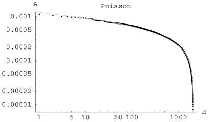
Figure 1: Rank-ordering of the circular voids in a random set of $10\hskip 1.0pt000$ points ($A$ is the void area and $R$ is the rank) compared with the predicted law (gray line).

To test the scaling of voids, we have applied the void-finder to several samples of random Cantor-like fractals. We show in Fig. 2 the results corresponding to a random sample of $10\hskip 1.0pt000$ points of a two-dimensional random Cantor-like fractal with $D=1.585$ and compare them with the expected Zipf law, $r\sim R^{-1/D}$ [24]. Note that the found circular voids (Fig. 2, top) do not cover the entire sample region (the unit square). In fact, they cover only 70% of it. Nonetheless, they convey well the notion of a hierarchy of voids. The application of this void-finder to multifractal samples is explained in Sects. 6.3.

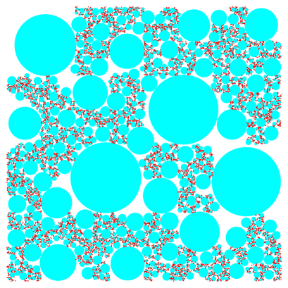
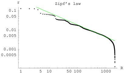
Figure 2: (Top figure) Random Cantor-like fractal sample with $10\hskip 1.0pt000$ points ($D=1.585$) and its corresponding voids found with the new algorithm (described in the text). (Bottom figure) Log-log plot of the rank-ordering of the void radii, compared with the straight line with slope $1/D$.

5 Geometry and scaling of voids in a monofractal

In this section, we study the geometry of voids in monofractals and prepare the generalization to multifractals. Our ultimate goal is to formulate a fractal model of voids in accord with a cosmic web structure. We consider the matter distribution to be continuous, unless the contrary is explicitly stated. The detailed treatment of continuous distributions requires some basic notions of geometry that we now recall, for we use them in this section and the following sections. These notions are necessary, in particular, to understand the intricate geometry of fractal voids.

In Euclidean space, the boundary of a region is defined as the set of points such that any ball centered on them intersects both the region and its complement. A region is closed if it contains its boundary. Normally, fractals live in closed sets that just consist of boundary points. A region is open if it does not contain any boundary point. In consequence, the complement of an open set is closed and vice versa. The union of open sets is open. The largest open part of a region is called its interior. A region is connected if it cannot be divided into two parts such that each one is disjoint with the boundary of the other. A region is convex if it contains every segment with ends inside it. Finally, a set is called dense if it intersects every open set.

Scaling of voids is natural in a strictly self-similar fractal: given that the fractal is the union of a number of smaller similar copies of itself, every void is reproduced on smaller scales, in an infinite hierarchy. Mandelbrot [10] expressed the similarity of voids as the diameter-number relation $N_{>}(\delta)\sim\delta^{-D}$, where the diameter of a void is the greatest distance between its points. Using the rank $R(\delta)=N_{>}(\delta)$, we can write the diameter-number relation as the Zipf law $\delta(R)\sim R^{-1/D}$. Random fractals can only be self-similar in a statistical sense, and then voids should adjust to the Pareto probability law $\mathbb{P}_{>}[\delta]=(\delta_{0}/\delta)^{D}$, with $\delta_{0}$ being the diameter lower cutoff. This law is indeed fulfilled by construction in one-dimensional Lévy flights, as seen in Sect. 3.4. In higher dimensions, the geometric construction of cut-out fractals produces a large class of fractals that are not strictly self-similar but fulfill a form of the Zipf law [10, 43, 44]. We review this construction as a model of the cosmic foam in Sect. 5.1, and we also consider the scaling of voids in general monofractals. In Sect. 5.2, we introduce the generalization to non-uniform cut-out fractals, as cosmic web models. Non-uniform cut-out fractals directly connect with multifractals, which are the subject of Sect. 6.

5.1 Cut-out fractals and cosmic foam

A cut-out set is obtained by removing an infinite sequence of disjoint connected open regions from an initial region that is bounded, closed and convex. Furthermore, for the set to be fractal, with vanishing volume, the sum of the volumes of the removed regions must tend to the volume of the initial region [10, 43]. Strictly speaking, every closed set is a cut-out set, because its complement is open and, therefore, is the union of a sequence of disjoint connected open regions. But it is natural to demand that proper cut-out fractals have infinite sequences of cutouts (voids). In one dimension, voids are necessarily open intervals, and every cut-out fractal can be constructed like the Cantor set, namely, by removing an infinite sequence of open intervals. Of course, this sequence does not need to be strictly self-similar. For example, the sequence of voids in a Lévy flight is only statistically self-similar.

In higher dimensions, a connected open region can have a very complicated shape; for example, it can surround any number of “islands” and have a rough boundary (like the shape of a cloud). If we restrict ourselves to cut-out fractals with convex voids and we further demand that these voids do not degenerate to lower dimensional objects along the sequence, this sequence must scale in a precise sense [44] (without being strictly self-similar). The scaling can be expressed as a particular power-law form of the rank order of diameters: $\delta(R)\asymp R^{-1/D_{\rm b}}$, in terms of the relation $\asymp$, which means that the quotient between the related quantities is bounded above and below. This number-diameter relation is equivalent to a common form of Zipf’s law: the log-log plot of the rank ordering stays between two parallel lines with slope given by the exponent ($-1/D_{\rm b}$, in the present case). Of course, since the sequence of voids is non-degenerate, namely, the void volume $V\asymp\delta^{3}$, we can also express the rank-ordering as

$$V(R)\asymp R^{-3/D_{\rm b}}.$$ (21)

A cut-out fractal with non-degenerate convex voids is formed by the union of the boundaries of its voids. Thus, this type of fractals formalizes the geometry of fractal foams. Regarding the cosmic structure, the first structures formed are actually sheets or walls (Zeldovich’s “pancakes”) [46]. The sheets form as the result of adhesive gravitational clustering: the initial under-dense regions expand and become depleted while the walls between them concentrate their mass, forming a foam. In fact, foam models of the cosmic structure have been proposed years ago. In particular, let us mention the Voronoi foam model by Icke and van de Weygaert [47]. It is natural to attribute to the cosmic foam statistical self-similarity, which should manifest itself in the void rank-ordering law (21).

We must examine if Eq. (21) still holds when we only consider spherical voids, namely, the rank-ordered sequences of non-overlapping spherical voids produced by our void-finder (e.g., the sequence of voids in Fig. 2). In a cut-out fractal, each spherical void must fit in one of its natural voids. The radius of the largest fitting sphere defines the inradius of the void. If we denote this inradius by $r$, we have that $r\asymp\delta$, for the sequence of voids is non-degenerate. Therefore, Eq. (21) still holds for the rank-ordered sequences of non-overlapping spherical voids.

Finally, we consider rank-ordered sequences of voids in a fractal that is not constructed as a cut-out set. We can deal with this case by endowing the fractal with a sort of “cut-out structure”, namely, by packing the complement of the fractal with open sets. The geometry of the complement of a fractal and its packing has been studied by Tricot [48, 49]. He proves a result equivalent to Eq. (21), under several conditions on the sequence of open sets. One important condition is the non-degeneracy of the sequence, in the sense explained above. Another condition applies to the shape of voids and is more general than convexity. And the condition that is crucial in the present case is that voids must be close to the fractal, namely, the quotients of their distances to the fractal by their diameters must be bounded. This latter condition is certainly satisfied if the voids always touch the fractal.

5.2 The cosmic web as a non-uniform cut-out fractal

Let us consider a cut-out set supported on the boundaries of its voids but with a non-uniform mass distribution on them. We regard it as an improved model of the cosmic fractal foam that arises from adhesive clustering: the foam evolves with the motion of the matter in the walls towards their intersections to form filaments, and the motion along the filaments to form nodes, resulting in a very non-uniform distribution. This distribution of sheets, filaments and nodes is called the cosmic web.

For illustrating the structure of non-uniform cut-out fractals, we construct a non-uniform fractal foam toy model that we call the Cantor-Sierpinski carpet. The Cantor-Sierpinski carpet is based on the standard Sierpinski carpet and on the two-dimensional Cantor set that is the Cartesian product of two standard Cantor sets. The Sierpinski carpets constitute a famous class of self-similar cut-out fractals with regular voids. The standard triadic Sierpinski carpet is also constructed as a sort of two-dimensional generalization of the middle third Cantor set: from an initial square, the (open) middle sub-square of side one third is cut out, and the iteration proceeds with the remaining eight sub-squares [10]. This fractal has dimension $D=1.89$.

We construct the Cantor-Sierpinski carpet using a modified algorithm. The first step still consists in cutting out the middle sub-square, an operation that we can describe as a uniform displacement of mass from that sub-square to the eight surrounding sub-squares. Then, to simulate the latter mass displacement along cosmic foam walls, we further concentrate part of the mass in the four sub-squares at the corners. Thus, the fractal generator consists in the division of the total mass into the nine sub-squares such that the central one receives nothing, the four sub-squares at the corners each receive a proportion $p_{1}$ of the total, and the remaining four sub-squares each receive a proportion $p_{2}<p_{1}$, with $4(p_{1}+p_{2})=1$. The resulting non-uniform cut-out fractal is supported on the Sierpinski carpet but has the highest concentrations of mass in the two-dimensional Cantor set: The case $p_{1}=1/6,\,p_{2}=1/12$ is shown in Fig. 3. Non-uniform fractal foams are actually multifractals.

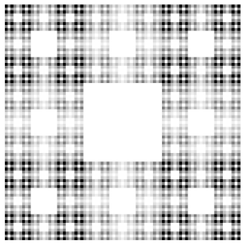
Figure 3: Two-dimensional non-uniform fractal foam: the Cantor-Sierpinski carpet. It is a multifractal cut-out set: beside the empty voids corresponding to the Sierpinski carpet, we can perceive very low density regions, in contrast with the mass concentrations near the two-dimensional Cantor dust.

6 Voids in a multifractal

In a multifractal, the mass in a ball of radius $r$ centered on a point $x$ decreases as a power of $r$, with a local exponent $\alpha(x)$ that varies with the point [40, 11]. $\alpha(x)$ is well defined for every point such that the mass in any ball centered on it is non-vanishing. The points that fulfill this condition form the support of the distribution, which is necessarily a closed set. The density at $x$ is proportional to the $\lim_{r\rightarrow 0}r^{\alpha(x)-d}$, where $d=3$ is the dimension of the ambient space. Points with $\alpha(x)<d=3$ are singular mass concentrations (the density diverges at the point $x$). In a multifractal model of cosmic structure, it is natural to identify these mass concentrations with dark matter halos [29, 18]. There are also points with $\alpha(x)>3$, belonging to mass depletions, which we study next (Sect. 6.1).

A multifractal is formed by the union of the sets of points with given local dimension $\alpha$. The multifractal spectrum $f(\alpha)$ gives the dimension of the set of points with local dimension $\alpha$. It is also useful to introduce its Legendre transform $\tau(q)=\inf_{\alpha}\left[q\,\alpha-f(\alpha)\right]$, which is the scaling exponent of $q$-moments. Hence, one derives the Rényi dimensions $D(q)=\tau(q)/(q-1)$, related to information measures. $D(0)$ is the box-counting dimension $D_{\rm b}$ of the distribution’s support and can be identified with the maximum of $f(\alpha)$. A monofractal (or unifractal) is the particular case in which the local dimension $\alpha$ is constant throughout its support and, therefore, $f(\alpha)=\alpha=D(q)$. In other words, a monofractal is a uniform mass distribution on a fractal support. This uniformity implies that statistical moments fulfill the hierarchical relation ${\bar{\mu}}_{k}\sim{{\bar{\mu}}_{2}}^{k-1}$ (Sect. 3.1), whereas in multifractals ${\bar{\mu}}_{k}\gg{{\bar{\mu}}_{2}}^{k-1}$ [18].

Naturally, the notion of a void is more complicated in multifractals than in monofractals. We can actually distinguish two types of voids.

6.1 The two types of voids in a multifractal

In Sect. 5, we have defined a void as a connected open region that contains no mass. However, this definition is, in a sense, too restrictive. Indeed, it should suffice for a point to belong to a void that the density vanishes at it. Thus, we can define the void region as the set of points with vanishing density. Since the density vanishes in open voids, this definition is more general. One might think that the density can only vanish, besides in open voids, in sets of null volume such as isolated points, curves or surfaces; but there are other possibilities. In a multifractal, most points can have local dimension $\alpha>3$ and, therefore, vanishing density. Unlike the points in open voids, those points belong to the support of the distribution and they form mass depletions inside it. Provided that the support of a multifractal has non-vanishing volume, its mass depletions normally occupy most of that volume.

Therefore, we can distinguish two types of voids in multifractal distributions: (i) open empty regions, forming the complement of the distribution’s support, and (ii) mass depletions formed by points with $\alpha>3$ which belong to the distribution’s support. As a multifractal with both types of voids, let us consider a non-uniform fractal foam, for example, the Cantor-Sierpinski carpet in Fig. 3. The totally empty squares in this figure are fractal voids of the first type. They follow the Zipf law (21) with an exponent given by the box-counting dimension $D_{\rm b}$ of the distribution’s support (the Sierpinski carpet). In this support, there are very low density regions, which are shown in light grey in Fig. 3. In the limit of infinite iterations, the low density regions become voids of the second type, with $\alpha>d=2$ and vanishing density.

Since voids of the first type are typical of monofractals, we regard only voids of the second type as proper multifractal voids. Multifractals with $D_{\rm b}<d$ have fractal support and, therefore, the voids of the second type occupy vanishing volume. But these voids become important when $D_{\rm b}=d$ and there are no voids of the first type. The case $D_{\rm b}=d$ is already studied in Sect. 3.4 as the case in which the void probability function vanishes in the continuum limit, corresponding to a non-lacunar fractal.

In this regard, we notice that the multifractal analysis of cosmological $N$-body simulations suggests that the value of $D(0)=D_{\rm b}$ is close to three [15, 16, 17]. Our recent analysis of simulations of cold dark matter [18] or of cold dark matter plus baryons [19] confirm it. Indeed, the supports of the distributions generated in $N$-body simulations seem to be their entire regions of definition, that is to say, the distributions appear non lacunar.

Let us analyze further the structure of non-lacunar multifractals. It is easy to realize that the geometry of proper multifractal voids is very intricate. Note that all their points are boundary points, since these voids have no interior. Let us identify every connected component with an individual void and assume that their number is countable, that is to say, they can be arranged in a sequence. In spite of belonging to a scaling distribution, these voids cannot satisfy the Zipf law (21), for it would imply that the total volume of the voids $\sum_{R}V(R)$ diverges (since $D_{\rm b}=3$). On the other hand, we can have an uncountable number of individual voids, unlike in the case of open voids. If there is an uncountable number of voids, every individual void can have zero volume, in spite of their total volume being positive. This happens, for example, in the mass distribution produced by the one-dimensional adhesion model (ruled by the Burgess equation with random initial conditions) [22]. The cosmic web produced by the three-dimensional adhesion model [21] is a complex multifractal [22, 23], whose geometrical features are not well understood yet.

One way to simplify the geometry of proper multifractal voids is to smooth the density field, as we do in the next section. In Sect. 6.3, we consider discrete multifractal samples and their empty spherical voids.

6.2 Voids as under-dense regions

Shandarin, Sheth & Sahni [7] and Sheth & van de Weygaert [8] define voids as under-dense regions of a continuous density field. The former authors further require that a void be connected. In general terms, under-dense regions are mass depletions, but they do not have the specific meaning that we have given to mass depletions in multifractals. Moreover, a multifractal does not define a regular density field, because the density diverges in mass concentrations. To remove these singularities, the density field must be smoothed. For example, it can be smoothed by using a window function or a low-pass filter of wave-numbers. In particular, the lognormal model employed in Sect. 3 can be understood as a coarse-grain approximation to a multifractal [41, 18]. A coarse-graining procedure is also necessary to recover a continuous distribution from a sample of it. Thus, it is used by Shandarin, Sheth & Sahni [7] to find voids in finite samples without having to consider the problem of shapes discussed in Sect. 4.

Let us see how the geometry of multifractal mass depletions changes under coarse-graining. A suitable coarse-graining process produces a continuous density field. If we define voids as the sets of points where the density is strictly smaller than a given value, say the average density, then the voids are open. Thus, multifractal mass depletions become like the monofractal voids defined in Sect. 5, although these multifractal voids are not empty. The entire under-dense region is also formed by a sequence of connected open regions (individual voids). As remarked in Sect. 5, connected open region can have very complex shapes. But their geometry is simpler than the geometry of proper multifractal voids which we have briefly explained in the preceding section.

For example, we have computed the iso-density level corresponding to the average density (one) of a realization in a square of a two-dimensional lognormal field with $\sigma=1.65$ and we have plotted it in Fig. 4. The black region is the under-dense region, which can be decomposed into a set of connected regions that constitute individual voids. A good part of the total volume belongs to the largest void, which percolates through the square. There are smaller voids as islets inside the matter clusters (“voids in clouds”). Unlike in a Gaussian density field, there is no symmetry between clusters and voids: the matter clusters contain most of the mass (80%) but occupy a small volume (20%). Thus, the average density in the voids is small, although they are not empty.

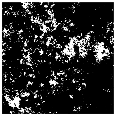
Figure 4: Voids defined by the under-dense region of a lognormal distribution (in black).

We can imagine the geometry of voids of the second type from the extrapolation of Fig. 4 to shrinking coarse-graining lengths: more and more matter halos pop up in the voids and more and more voids pop up in the matter clusters. In the limit of vanishing coarse-graining length, the halos are fully mixed with (are dense in) the voids. This picture agrees with the result of re-simulating with higher resolution voids in $N$-body simulations in Ref. [6]. Moreover, as the distribution becomes more singular, voids occupy an increasing fraction of the total volume that tends to one and contain a decreasing fraction of the total mass that tends to zero. Despite the large volume of this type of voids, their shape is such that no circle, however small, can fit inside them (which is equivalent to stating that they have no interior).

6.3 Statistics of spherical voids in multifractal samples

Let us show that the statistics of the spherical voids in a finite multifractal sample provide a good indication of the type of voids. We first consider lacunar multifractals, namely, multifractals with fractal support or, in other words, with voids of the first type. In finite samples of these multifractals, the size of the largest voids is hardly dependent on the density of points $n$. Furthermore, the sizes of voids scale. All this follows from the analyses in Sect. 3.4, Sect. 5 and Sect. 6.1, but it is also intuitively obvious by examining Figs. 2 and 3.

For the study of the statistics of spherical voids in non-lacunar multifractals, we use a random multinomial multifractal supported on the full unit square. Its correlation dimension is $D_{2}=1.526$ and its homogeneity scale $r_{0}=1$ (the edge of the unit square). We define this multifractal with great precision, namely, with linear resolution $2^{24}\simeq 1.7\cdot 10^{7}$, and we generate a random sample of it with $10\hskip 1.0pt000$ points (the typical order of magnitude of galaxy volume-limited samples). The spherical voids in this sample are obtained by applying the void-finder of Sect. 4. We find some relatively large voids (see Fig. 5). The largest void has a radius equal to 0.0484 and an area equal to 0.00736 (in box-size units). According to the results of Sect. 2.1, the expected number of voids of at least that size, in a sample of the uniform distribution with $10\hskip 1.0pt000$ points and such that $N=73.6$, would be $10\hskip 1.0pt000\,(12\pi^{2}/35)73.6^{2}\exp(-73.6)\simeq 2\cdot 10^{-24}$. Therefore, the largest void is too large for a Poisson distribution.

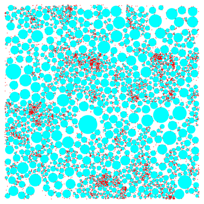
Figure 5: $10\hskip 1.0pt000$ point sample of a random multifractal supported in the full unit square, with its corresponding voids (top figure). Log-log plot of the rank-ordering of the void radii (bottom plot).

But the largest void is sensibly smaller than the homogeneity scale. For this non-lacunar fractal, we can use the estimate of the largest void size based on the lognormal distribution that is obtained in Sect. 3.3. It is also valid in two dimensions. In fact, we have obtained precisely $N=73$ for $N_{\rm t}=10\hskip 1.0pt000$ points and $\sigma=1$. This value of $\sigma$ is slightly larger than the actual value, $\sigma=0.82$, which can be calculated from the point density variance at the scale of the size of the void. However, estimates obtained from $P_{0}[V]$ are always lower estimates, so we conclude that the lognormal distribution provides a reasonable model of the largest void sizes in this multifractal.

In regard to the rank-ordering of the sequence of sizes of the spherical voids in this multifractal sample, it does not fulfill Zipf’s law, as shown in Fig. 5. In fact, its aspect is similar to the aspect of the plot that corresponds to a Poisson distribution (Fig. 1).

We have also tested samples of the same multifractal with larger numbers of points. Naturally, the largest voids are smaller in larger samples. Thus, it becomes clear that the size of the largest void bears no relation to the homogeneity scale. Furthermore, the estimation of that size in Sect. 3.3 based on the lognormal distribution given by Eq. (19), in particular, still holds in larger samples.

7 Voids in cosmological simulations and galaxy samples

7.1 Voids in cosmological simulations

Here, we briefly study the statistics of spherical voids in data from cosmological $N$-body simulations, taking into account the conclusions of multifractal analyses of cosmological simulations [15, 16, 17, 18, 19]. We have remarked above that these analyses suggests that the box-counting dimension of the matter distribution is $D_{\rm b}=3$, making the fractal non-lacunar. However, the measure of lacunarity provided by $D_{\rm b}$ is rather inaccurate. Thus, it is worthwhile to study directly the distribution of voids.

The first observation that is relevant, although somewhat trivial, is that the spherical voids in state-of-the-art simulations, with many millions of particles, are very small in comparison with the simulated volume and with the scale of homogeneity as well. This observation suggests that the matter distribution is supported in the full simulated volume. To confirm it, we can measure how the size of the largest void changes with the density of points $n$. For example, we take the redshift-zero particle distribution in the GIF2 simulation, which has a relevant scaling range, up to the homogeneity scale $r_{0}=1/4$ (in box-size units) [18]. We extract two random samples from this particle distribution, with $N_{\rm t}=10\hskip 1.0pt000$ and $100\hskip 1.0pt000$ points, respectively. In the first one, the largest void has a radius equal to 0.097 and a volume equal to 0.0038 (in box-size units). In the $100\hskip 1.0pt000$ point sample, the largest void has a radius equal to 0.059 and a volume equal to 0.00086. This pattern of shrinking of the largest void is consistent with a non-lacunar multifractal.

Of course, the largest void in a small sample contains particles of any larger sample. In general, a relevant question in the process of obtaining better samples (with larger $n$) is if and how it affects voids. The process cannot alter voids of the first type significantly, but its effect on proper multifractal voids is like the effect of a shrinking coarse-graining length described in Sect. 6.2. Therefore, a more general and definite proof of non-lacunarity in cosmological simulations is provided by the method of Gottlöber et al [6], consisting in re-simulating with higher resolution voids found in $N$-body simulations. The result of this method is that new structure arises inside these voids in a self similar pattern, just like a non-lacunar fractal predicts.

7.2 Voids in galaxy samples and galaxy bias

There are many studies of the various aspects of galaxy voids. The studies that are most relevant in our context have been carried out by Tikhonov and Karachentsev [25, 26, 27]. They study the statistics of voids in several galaxy samples and find evidences of scaling of galaxy voids. As we have shown, scaling of voids is the hallmark of a lacunar fractal. Here, we re-analyze Tikhonov’s data from the 2dF survey [26] in regard to the size of the largest void and, especially, to the possible scaling of its voids.

Tikhonov [26] selects from the 2dF survey a volume limited sample (VLS) with 7219 galaxies, such that the volume per galaxy is 513 Mpc³ $h^{-3}$. The largest void in it corresponds to a sphere with radius 21.3 Mpc $h^{-1}$ and volume $4.05\cdot 10^{4}$ Mpc³ $h^{-3}$. Thus, if the sample belonged to a uniform distribution, the expected number of sample galaxies in that sphere would be 79. Then, the expected number of voids of that size, according to Sect. 2.1, would be $7219\,(12\pi^{2}/35)\,79^{2}\,e^{-79}=8\cdot 10^{-27}$, that is, absolutely negligible. However, the value $N=79$ is reasonable for a non-lacunar fractal, according to Sect. 3.3.

Tikhonov [26] rank-orders the void sizes in the 2dF VLS and concludes that there is a scaling range. This scaling range is about a decade, namely, an order of magnitude in the rank (from rank 60 to rank 600, approximately). Tikhonov uses his own void-finder, which first fits the largest empty spheres and then applies a merging criterion (in a similar way to El-Ad & Piran [5]). We use our void-finder (defined in Sect. 4) to just find the list of non-overlapping spherical voids in Tikhonov’s VL sample. The resulting rank order is plotted in Fig. 6. The range of radii is nearly the same range found by Tikhonov but no scaling can be discerned. The rank order shown in Fig. 6 is similar to the ones that we found in Ref. [24], and they all are actually typical of non-lacunar fractals; namely, they all are similar to the rank-ordering of Poisson voids (Fig. 1), but they span longer ranges of sizes.

Figure 6: Rank-ordering of the voids in a 2dFGRS sample with $7\hskip 1.0pt000$ galaxies ($r$ is the void radius in Mpc $h^{-1}$). This rank-ordering is typical of non-lacunar fractals.

Actually, the analyses of voids that attempt to find the Zipf law have been motivated by the assumption of a lacunar fractal distribution of galaxies. We must reconsider this assumption, in regard to the evidences of a multifractal distribution of (dark) matter with $D_{\rm b}=3$ [18, 19] and the results of the preceding section. Indeed, a galaxy distribution that closely follows the full matter distribution is probably also non-lacunar. To actually determine the type of galaxy voids, we need to model the galaxy biasing.

Dark matter concentrations (halos) are the natural places for galaxy formation. These concentrations have been studied as peaks of a Gaussian density field [28]. In contrast, our model of galaxy biasing stems from the definition of halos as over-dense regions of a coarse-grain multifractal density field in Sect. 6.2. As emphasized there, this type of density field is very different from a Gaussian field on nonlinear scales. The main difference is the strong asymmetry between over-dense and under-dense regions: the former occupy a small volume but contain most of the mass. Therefore, we do not need a high density threshold to define clustered mass concentrations, but just the average density. We can assign a galaxy to every coarse-grain mass concentration (halo), obtaining a clustered distribution with a minimal bias.

The average density corresponds to the local dimension $\alpha=3$, which separates mass concentrations ($\alpha<3$) from mass depletions ($\alpha>3$). Naturally, we can set a higher density threshold to differentiate one highly clustered and luminous population of galaxies (“wall galaxies”) from another more homogeneous and less luminous population (“field galaxies”). A natural choice of threshold should be the density that corresponds to the local dimension $\alpha_{1}$ of the mass concentrate [18], because halos with smaller densities contain relatively little mass. Notice the analogy with the procedure of El-Ad & Piran [5] in the “wall builder” phase of their void-finder. With this prescription, the voids in the “wall galaxies” contain “field galaxies”. However, the distribution of these “field galaxies” is not homogeneous and they tend to avoid the central parts of voids. The most homogeneous halo subpopulation consists of halos with $\alpha$ close to three, with so little gas that it may not form galaxies. Peebles [30] discusses the nature of void objects and argues that the formation of observable objects is suppressed in voids, to the extent that it may constitute a challenge to our current structure formation paradigm. However, Furlanetto & Piran [50] use an excursion set model and conclude that the size of voids diminishes with the galaxy luminosities in reasonable agreement with observations. Our multifractal model is in accord with this conclusion.

8 Summary and Conclusions

We have developed statistical methods for the study of cosmic voids and we have applied them to various distributions of observable objects. The method of choice depends crucially on the number density $n$ of objects. If the density is sufficiently small for having a small number of objects in a volume in which the Universe is homogeneous, then the objects are weakly correlated and the analysis for Poisson voids in Sect. 2 is relevant. Of course, this case is the most amenable to analytical methods. We have found the distribution of spherical voids and the volume of the largest void, and we have shown how to generalize these results to more general shapes of voids. Not surprisingly, to observe a really large void, namely, with volume $V\gg 1/n$, one needs an exponentially large sample, with a number of objects $N_{\rm t}\sim e^{nV}$. And this sample could only come from surveying volumes exponentially larger than the homogeneity volume.

The conclusion is that the voids observed in galaxy surveys, for example, are not due to Poissonian fluctuations. Indeed, galaxy samples have had for long time number densities such that there are many galaxies in a homogeneity volume. The objects inside a homogeneity volume have correlations, which are necessary for the existence of voids but make the application of analytical methods more difficult. For still moderate $n$, an expansion in powers of $n$ yields general results and, in particular, yields a formula for the distribution of voids, although the computations are hardly feasible. It is preferable to resort to significant models that are valid for any $n$. We have focused on a hierarchical Poisson model and on the lognormal model, which illustrate two different behaviors of the largest voids.

We define the hierarchical Poisson model by restricting the support of a Poisson distribution to random clusters. Thus, we construct a point distribution that saturates the general moment inequality ${\bar{\mu}}_{k}\geq{{\bar{\mu}}_{2}}^{k-1}$. When ${\bar{\mu}}_{2}\gg 1$, the clusters are small and the distribution is strongly correlated, but then its large voids are just the voids in the random distribution of clusters. These voids are independent of the magnitude of the density of objects inside clusters. Therefore, the distribution of the volume of the largest void is of Fréchet-Pareto type, in contrast with the pure Poisson case, in which the largest void vanishes when $n\rightarrow\infty$ (Gumbel type).

It is natural to understand the hierarchical Poisson model as a real hierarchy of clusters of clusters in a self-similar pattern. Thus, it becomes a fractal model with hierarchical and scaling correlation functions. For example, one-dimensional Lévy flights are constructed so as to have scaling voids that follow the Pareto distribution. In contrast, the study of voids in higher-dimensional fractals demands a good deal of geometry. A convenient approach to fractal voids is the construction of cut-out fractals. In particular, a fractal foam is a possible model of the sheet structure of the cosmic web. Fractal foams have voids with simple shapes and scaling sizes. These properties of voids can be generalized to other monofractal distributions.

A monofractal distribution is characterized by its box-counting dimension $D_{\rm b}$ and is essentially uniform throughout its support, like the hierarchical Poisson model. However, the adhesive gravitational dynamics gives rise to non-uniform distributions that contain filaments and nodes, in addition to sheets. This motivates us to consider non-uniform fractal foam models and, ultimately, multifractal models of the cosmic web. A multifractal is characterized by a spectrum of dimensions, but its box-counting dimension still plays the most significant role in regard to voids. If $D_{\rm b}<3$, then the support of the multifractal has vanishing volume, namely, is itself a fractal set. Therefore, the distribution of voids is independent of the non-uniformity of the matter distribution inside its support. A more interesting type of multifractal voids arises in the case that $D_{\rm b}=3$ and the support is the total volume.

Multifractals with support in a full volume have been called non-lacunar fractals by Mandelbrot [10]. Whether or not non-lacunar fractals have voids is a subtle question. Certainly, they have no voids with empty interior in which one can fit an empty sphere. However, they do have sets of mass depletions with large volumes in which the density vanishes. We have called them voids of second type. The lognormal model provides us with a good description of the statistics of this type of voids as they appear in a multifractal sample with number density $n$. We deduce, for example, that the volume of the largest spherical void is much larger than in a Poisson distribution but is still small in comparison with the homogeneity scale (its distribution is actually of Gumbel type). On the other hand, these voids do not have scaling sizes. A more geometrical picture of this type of voids is achieved by representing them as under-dense regions of a smoothed density field (Sect. 6.2). Thus, second type voids become geometrically similar to first type voids, although they necessarily contain mass. This mass is part of self-similar structures that can be observed as the smoothing length shrinks and the resolution increases.

Indeed, it has been observed by Gottlöber et al [6] in cosmological $N$-body simulations that a pattern of self-similar structure arises inside voids when the resolution increases. Further statistical evidence supports that the voids in cosmological simulations belong to a non-lacunar fractal (Sect. 7.1). Therefore, we can assert that dark matter voids are well described as second type voids in a non-lacunar fractal.

It is less certain that a similar description is appropriate for galaxy voids. Admitting that the distribution of galaxies is fractal in the relevant range of scales, we have examined the observational and theoretical arguments for lacunarity. Scaling of galaxy voids implies lacunarity. We have not found this scaling, neither in Ref. [24] nor in Sect. 7.2, in spite of the favorable results of Tikhonov and Karachentsev [25, 26, 27]. Another argument for lacunarity is the emptiness of voids. Peebles argues that the formation of observable objects is suppressed in voids [30]. But it rather seems that the size of voids diminishes with the galaxy luminosities [50]. This is also predicted by a non-lacunar multifractal model of galaxy bias in which the mass (or luminosity) of galaxies is ruled by the local dimension as a measure of mass concentration (Sect. 7.2). However, very weak concentrations may not form galaxies and remain inside voids as dark matter halos. This might produce a low lacunarity in the distribution of galaxies.

As regards the formation of voids, we have introduced multifractal models of the adhesion-like dynamics that gives rise to the cosmic web. However, to obtain non-lacunar foams, we must modify slightly the construction introduced in Sect. 5.2; namely, we must require that the initial under-dense regions become depleted but not empty. This is necessary to obtain the proper cosmic web structure. However, the construction of a realistic model of the formation of voids along these lines is beyond the scope of this work.

In conclusion, a good description of cosmic voids and, in general, the structure of matter is provided by a non-lacunar multifractal, with dimension $D_{\rm b}=3$ (the dimension of non-fractal distributions) and without empty voids (first-type voids). The distribution of galaxies is probably non-lacunar as well, but it could have a low lacunarity. The peculiar structure of non-lacunar fractals can be partly responsible for the controversy about the application of fractal geometry to the distribution of galaxies. Indeed, that structure is very different from the structure of monofractals (or multifractals with $D_{\rm b}<3$) that has been normally assumed for the distribution of galaxies.

Appendix A The four point integral

To prove Eq. (1) and evaluate the function $f$ therein and its integral, we need the explicit expression of the change of Cartesian coordinates to coordinates adapted to the sphere defined by the four points. We first express each point as the sum

$$x_{i}=x_{\mathrm{c}}+ru_{i}\,,$$

where $x_{\mathrm{c}}$ is the center of the sphere, $r$ is its radius and, therefore, the vectors $u_{i}$ are unitary; namely,

$$u_{i}=(\sin\theta_{i}\cos\phi_{i},\sin\theta_{i}\sin\phi_{i},\cos\theta_{i}),$$

in standard spherical coordinates. The transformation of the twelve coordinates $\{(x_{i}^{1},x_{i}^{2},x_{i}^{3})\}_{i=1}^{4}$ to the twelve coordinates $\{(x_{\mathrm{c}}^{1},x_{\mathrm{c}}^{2},x_{\mathrm{c}}^{3}),r,\{{\mbox{\boldmath{$\theta$}}}_{i}\}_{i=1}^{4}\}$, where ${\mbox{\boldmath{$\theta$}}}_{i}=(\theta_{i},\phi_{i})$, introduces the Jacobian matrix of the transformation. For elementary reasons of symmetry, the transformation of the four point volume element can be expressed as

$$d^{3}x_{1}\,d^{3}x_{2}\,d^{3}x_{3}\,d^{3}x_{4}=\\ d^{3}x_{\rm c}\,r^{8}dr\,g({\mbox{\boldmath{$\theta$}}}_{1},{\mbox{\boldmath{$\theta$}}}_{2},{\mbox{\boldmath{$\theta$}}}_{3},{\mbox{\boldmath{$\theta$}}}_{4})\,d^{2}{\mbox{\boldmath{$\theta$}}}_{1}\,d^{2}{\mbox{\boldmath{$\theta$}}}_{2}\,d^{2}{\mbox{\boldmath{$\theta$}}}_{3}\,d^{2}{\mbox{\boldmath{$\theta$}}}_{4},$$

where $d^{2}{\mbox{\boldmath{$\theta$}}}=\sin\theta\,d\theta\,d\phi$ is the surface element on the unit sphere and $g$ is an unknown symmetric function. Therefore, the calculation of the Jacobian determinant is reduced to the calculation of this function.

The expansion of the Jacobian determinant produces $12!=479\hskip 1.0pt001\hskip 1.0pt600$ terms. Although the Jacobian matrix has many vanishing terms, the number of non-vanishing terms in the expansion of its determinant is huge nonetheless and a direct calculation is awkward. It is convenient to use the formalism of exterior algebra, which provides a suitable way to organize the calculation. We begin with writing

$$dx_{i}^{a}=dx_{\mathrm{c}}^{a}+u_{i}^{a}dr+rdu_{i}^{a}\,,$$

and, then, we can calculate the one-point volume element as the wedge product

$$dx_{i}^{1}\wedge dx_{i}^{2}\wedge dx_{i}^{3}=dx_{\mathrm{c}}^{1}\wedge dx_{\mathrm{c}}^{2}\wedge dx_{\mathrm{c}}^{3}+\cdots+r^{2}\,dr\wedge d^{2}{\mbox{\boldmath{$\theta$}}}_{i}\,,$$

where the dots stand for the eighteen remaining terms. The total number of terms is the number of triplets of the six coordinates $\{(x_{\mathrm{c}}^{1},x_{\mathrm{c}}^{2},x_{\mathrm{c}}^{3}),r,{\mbox{\boldmath{$\theta$}}}_{i}\}$ with no repeated coordinates, namely, $C^{6}_{3}=20$.

The wedge product $\wedge_{i=1}^{4}(dx_{i}^{1}\wedge dx_{i}^{2}\wedge dx_{i}^{3})$ could give rise to many terms, but most terms in the one-point volume element do not contribute to it: for example, we can deduce from the structure of the final result that, in the volume element of index $i$, only the terms proportional to $d^{2}{\mbox{\boldmath{$\theta$}}}_{i}$ can contribute. We note that the four-point wedge product is oriented and one must take its absolute value for the function $g$ to be positive and symmetric. After a lengthy calculation, one obtains

$$g({\mbox{\boldmath{$\theta$}}}_{1},{\mbox{\boldmath{$\theta$}}}_{2},{\mbox{\boldmath{$\theta$}}}_{3},{\mbox{\boldmath{$\theta$}}}_{4})=$$

$$|C\left(\theta_{3}\right)C\left(\phi_{2}\right)S\left(\theta_{1}\right)S\left(\theta_{2}\right)S\left(\phi_{1}\right)-C\left(\theta_{4}\right)C\left(\phi_{2}\right)S\left(\theta_{1}\right)S\left(\theta_{2}\right)S\left(\phi_{1}\right)-$$

$$C\left(\theta_{2}\right)C\left(\phi_{3}\right)S\left(\theta_{1}\right)S\left(\theta_{3}\right)S\left(\phi_{1}\right)+C\left(\theta_{4}\right)C\left(\phi_{3}\right)S\left(\theta_{1}\right)S\left(\theta_{3}\right)S\left(\phi_{1}\right)+$$

$$C\left(\theta_{2}\right)C\left(\phi_{4}\right)S\left(\theta_{1}\right)S\left(\theta_{4}\right)S\left(\phi_{1}\right)-C\left(\theta_{3}\right)C\left(\phi_{4}\right)S\left(\theta_{1}\right)S\left(\theta_{4}\right)S\left(\phi_{1}\right)-$$

$$C\left(\theta_{3}\right)C\left(\phi_{1}\right)S\left(\theta_{1}\right)S\left(\theta_{2}\right)S\left(\phi_{2}\right)+C\left(\theta_{4}\right)C\left(\phi_{1}\right)S\left(\theta_{1}\right)S\left(\theta_{2}\right)S\left(\phi_{2}\right)+$$

$$C\left(\theta_{1}\right)C\left(\phi_{3}\right)S\left(\theta_{2}\right)S\left(\theta_{3}\right)S\left(\phi_{2}\right)-C\left(\theta_{4}\right)C\left(\phi_{3}\right)S\left(\theta_{2}\right)S\left(\theta_{3}\right)S\left(\phi_{2}\right)-$$

$$C\left(\theta_{1}\right)C\left(\phi_{4}\right)S\left(\theta_{2}\right)S\left(\theta_{4}\right)S\left(\phi_{2}\right)+C\left(\theta_{3}\right)C\left(\phi_{4}\right)S\left(\theta_{2}\right)S\left(\theta_{4}\right)S\left(\phi_{2}\right)+$$

$$C\left(\theta_{2}\right)C\left(\phi_{1}\right)S\left(\theta_{1}\right)S\left(\theta_{3}\right)S\left(\phi_{3}\right)-C\left(\theta_{4}\right)C\left(\phi_{1}\right)S\left(\theta_{1}\right)S\left(\theta_{3}\right)S\left(\phi_{3}\right)-$$

$$C\left(\theta_{1}\right)C\left(\phi_{2}\right)S\left(\theta_{2}\right)S\left(\theta_{3}\right)S\left(\phi_{3}\right)+C\left(\theta_{4}\right)C\left(\phi_{2}\right)S\left(\theta_{2}\right)S\left(\theta_{3}\right)S\left(\phi_{3}\right)+$$

$$C\left(\theta_{1}\right)C\left(\phi_{4}\right)S\left(\theta_{3}\right)S\left(\theta_{4}\right)S\left(\phi_{3}\right)-C\left(\theta_{2}\right)C\left(\phi_{4}\right)S\left(\theta_{3}\right)S\left(\theta_{4}\right)S\left(\phi_{3}\right)-$$

$$C\left(\theta_{2}\right)C\left(\phi_{1}\right)S\left(\theta_{1}\right)S\left(\theta_{4}\right)S\left(\phi_{4}\right)+C\left(\theta_{3}\right)C\left(\phi_{1}\right)S\left(\theta_{1}\right)S\left(\theta_{4}\right)S\left(\phi_{4}\right)+$$

$$C\left(\theta_{1}\right)C\left(\phi_{2}\right)S\left(\theta_{2}\right)S\left(\theta_{4}\right)S\left(\phi_{4}\right)-C\left(\theta_{3}\right)C\left(\phi_{2}\right)S\left(\theta_{2}\right)S\left(\theta_{4}\right)S\left(\phi_{4}\right)-$$

$$C\left(\theta_{1}\right)C\left(\phi_{3}\right)S\left(\theta_{3}\right)S\left(\theta_{4}\right)S\left(\phi_{4}\right)+C\left(\theta_{2}\right)C\left(\phi_{3}\right)S\left(\theta_{3}\right)S\left(\theta_{4}\right)S\left(\phi_{4}\right)|\,\phantom{.},$$

where $C=\cos$ and $S=\sin$. The integral over the angles is simplified by taking into account the permutation symmetry. It yields

$$\int g({\mbox{\boldmath{$\theta$}}}_{1},{\mbox{\boldmath{$\theta$}}}_{2},{\mbox{\boldmath{$\theta$}}}_{3},{\mbox{\boldmath{$\theta$}}}_{4})\,d^{2}{\mbox{\boldmath{$\theta$}}}_{1}\,d^{2}{\mbox{\boldmath{$\theta$}}}_{2}\,d^{2}{\mbox{\boldmath{$\theta$}}}_{3}\,d^{2}{\mbox{\boldmath{$\theta$}}}_{4}=4!\,\frac{256\,\pi^{5}}{105}\,.$$

Finally, we can substitute the radius $r$ by the volume $V=4\pi r^{3}/3$, using $V^{2}dV=(4\pi/3)^{3}3r^{8}dr$. Therefore, the function $f$ defined in Eq. (1) is

$$f=\frac{3^{2}}{4^{3}\pi^{3}}g,$$

and its integral is

$$\int f({\mbox{\boldmath{$\theta$}}}_{1},{\mbox{\boldmath{$\theta$}}}_{2},{\mbox{\boldmath{$\theta$}}}_{3},{\mbox{\boldmath{$\theta$}}}_{4})\,d^{2}{\mbox{\boldmath{$\theta$}}}_{1}\,d^{2}{\mbox{\boldmath{$\theta$}}}_{2}\,d^{2}{\mbox{\boldmath{$\theta$}}}_{3}\,d^{2}{\mbox{\boldmath{$\theta$}}}_{4}=4!\,\frac{12\,\pi^{2}}{35}\,.$$

Appendix B Asymptotic expansions of the lognormal $P_{0}[V]$

Here we obtain the asymptotic expansions as $\sigma\rightarrow\infty$ or $N\rightarrow\infty$ of the integral in Eq. (13), namely,

$$\int\limits_{0}^{\infty}\exp\left[-\frac{(\ln r+\sigma^{2}/2)^{2}}{2\sigma^{2}}-Nr\right]\frac{dr}{r}\,.$$

An inspection shows that this integral is awkward for the standard methods of asymptotic expansion of Laplace integrals, based on Watson’s lemma and its generalizations [51]. Thus, we first transform the integral, using the following identity:

$$\exp\left[-\frac{(\ln r+\sigma^{2}/2)^{2}}{2\sigma^{2}}\right]=$$

$$\frac{\sigma}{\sqrt{2\pi}}\int\limits_{-\infty}^{\infty}dz\,\exp\left[-\frac{\sigma^{2}z^{2}}{2}+i\left(\ln r+\frac{\sigma^{2}}{2}\right)z\right]$$

Thus,

$$\int\limits_{0}^{\infty}\exp\left[-\frac{(\ln r+\sigma^{2}/2)^{2}}{2\sigma^{2}}-Nr\right]\frac{dr}{r} =$$

$$\frac{\sigma}{\sqrt{2\pi}}\int\limits_{-\infty}^{\infty}dz\,\exp\left[-\frac{\sigma^{2}z^{2}}{2}+i\frac{\sigma^{2}}{2}z\right]\int\limits_{0}^{\infty}\frac{dr}{r}\,e^{-Nr}r^{iz} =$$

$$\frac{\sigma}{\sqrt{2\pi}}\int\limits_{-\infty}^{\infty}dz\,\exp\left[-\frac{\sigma^{2}z^{2}}{2}+i\frac{\sigma^{2}}{2}z\right]N^{-iz}\,\Gamma(iz),$$ (22)

where the change of integration order is valid if the integrals are convergent. For the integral over $r$ to be convergent, we need that $\mathop{\rm Re}(iz)=-\mathop{\rm Im}(z)>0$.

To obtain the asymptotic expansion as $\sigma\rightarrow\infty$, it is convenient to choose $\mathop{\rm Im}(z)=1/2$ in the integral (22), namely, to define $z=\zeta+i/2$ with $\zeta$ real, for it removes the linear term in the exponential. In translating the integral (22) from $\mathop{\rm Im}(z)<0$ to $\mathop{\rm Im}(z)=1/2$, we pick up the residue at $z=0$ of the integrand (from the Gamma function):

$$\int\limits_{-i-\infty}^{-i+\infty}dz\,\exp\left[-\frac{\sigma^{2}z^{2}}{2}+i\frac{\sigma^{2}}{2}z\right]N^{-iz}\,\Gamma(iz)=$$

$$2\pi+e^{-\sigma^{2}/8}N^{1/2}\int\limits_{-\infty}^{\infty}d\zeta\,\exp\left[-\frac{\sigma^{2}\zeta^{2}}{2}\right]N^{-i\zeta}\,\Gamma\left(i\zeta-\frac{1}{2}\right)$$

This integral is suitable for standard methods of asymptotic expansion of general Laplace integrals [51]. They yield

$$\int\limits_{-\infty}^{\infty}d\zeta\,\exp\left[-\frac{\sigma^{2}\zeta^{2}}{2}\right]N^{-i\zeta}\,\Gamma\left(i\zeta-\frac{1}{2}\right)=\frac{\sqrt{2\pi}}{\sigma}\left(f(0)+\frac{1}{2\sigma^{2}}f^{\prime\prime}(0)+\cdots\right),$$

where $f(\zeta)=N^{-i\zeta}\,\Gamma\left(i\zeta-1/2\right)$. For the first term, we only need $f(0)=\Gamma(-1/2)=-2\sqrt{\pi}$.

To obtain the asymptotic expansion as $N\rightarrow\infty$, we write the integral (22) as

$$\int\limits_{-i-\infty}^{-i+\infty}dz\,\exp\left[-\frac{\sigma^{2}z^{2}}{2}+\left(\frac{\sigma^{2}}{2}-\ln N\right)iz\right]\Gamma(iz)\,,$$

and find the stationary point of the exponent, which occurs at

$$z=\left(\frac{1}{2}-\frac{\ln N}{\sigma^{2}}\right)i.$$

Let us call $\lambda=\ln N/\sigma^{2}-1/2$ and make the change of variable $z=\zeta-i\lambda$ with $\zeta$ real. Thus, $\mathop{\rm Im}(z)=-\lambda<0$ if $\lambda>0$, that is, if $\ln N>\sigma^{2}/2$, which is fulfilled in the $N\rightarrow\infty$ asymptotics. Therefore,

$$\int\limits_{-i-\infty}^{-i+\infty}dz\,\exp\left[-\frac{\sigma^{2}z^{2}}{2}+\left(\frac{\sigma^{2}}{2}-\ln N\right)iz\right]\Gamma(iz)=$$

$$e^{-\sigma^{2}\lambda^{2}/2}\int\limits_{-\infty}^{\infty}d\zeta\,e^{-\sigma^{2}\zeta^{2}/2}\,\Gamma(\lambda+i\zeta)$$

The asymptotic expansion as $\lambda\rightarrow\infty$ of the last integral is straightforward, for it requires only the standard asymptotic expansion of the Gamma function. After some lengthy algebra, it yields

$$\int\limits_{-\infty}^{\infty}d\zeta\,e^{-\sigma^{2}\zeta^{2}/2}\,\Gamma(\lambda+i\zeta)=\Gamma(\lambda)\frac{\sqrt{2\pi}}{\sigma}\exp\left[-\frac{(\ln\lambda)^{2}}{2\sigma^{2}}\right]\left[1+{\mathop{\rm O}\nolimits\left(\frac{\ln^{2}\!\lambda}{\lambda}\right)}\right].$$

Hence,

$$\int\limits_{-i-\infty}^{-i+\infty}dz\,\exp\left[-\frac{\sigma^{2}z^{2}}{2}+\left(\frac{\sigma^{2}}{2}-\ln N\right)iz\right]\Gamma(iz)\approx$$

$$\frac{2\pi\sigma}{\ln N}\exp\left\{-\frac{\ln^{2}\!N}{2\sigma^{2}}+\frac{\ln N}{2\sigma^{2}}\left[2\ln\left(\frac{\ln N}{\sigma^{2}}\right)+\sigma^{2}-2\right]-\frac{1}{2\sigma^{2}}\ln^{2}\left(\frac{\ln N}{\sigma^{2}}\right)-\frac{\sigma^{2}}{8}\right\}.$$

Appendix C The probability of voids in a Lévy flight

Lévy flights are analogous to Brownian random walks, but they are based on the Lévy stable distributions rather than on the normal distribution. Unlike this distribution, the Lévy stable distributions do not have finite variance and, in particular, the Lévy distributions that we consider here do not have finite mean. These distributions are defined for positive $x$ only and they have a probability function $P(x)$ with power-law asymptotic form $C/x^{D+1}$, where $C>0$ and $0<D<1$. Every Lévy distribution is characterised by these two parameters and we can substitute the amplitude $C$ by a scaling parameter $t$ such that the probability density $P_{t}(x)=t^{-1/D}P_{1}(t^{-1/D}x)$. The explicit expression of $P_{t}(x)$ is only known for a few values of $D$, chiefly, $D=1/2$, with $P_{t}(x)=\left(t/\sqrt{\pi}\right)\exp(-t^{2}/x)/x^{3/2}$. The cumulative probability of a Lévy distribution is just a function of $t^{-1/D}x$, namely, $P_{>}(t^{-1/D}x)$, with the parameter $D$ only, due to the scaling property of $P_{t}(x)$. In a Lévy flight $x(t)$ with dimension $D$, the increment $x(t)-x(s)$ has a Lévy distribution with parameters $D$ and $t-s$.

Brownian random walks are continuous but Lévy flights have jumps (hence their name). Mandelbrot [10] studies Lévy flight jumps and discusses its power-law distribution, namely, $\mathbb{P}_{>}[L]\propto L^{-D}$. He points out that $\mathbb{P}_{>}[L]$ is ill-defined as $L\rightarrow 0$ and explains that it must be understood as the cumulative conditional probability $\mathbb{P}[L>l|L>\lambda]=(\lambda/l)^{D}$. However, he does not include a proof of this very plausible equation. We include here a simple proof and a brief discussion, for the sake of completeness.

In general, we have that

$$\mathbb{P}[L>l|L>\lambda]=\frac{\mathbb{P}_{>}(l)}{\mathbb{P}_{>}(\lambda)},$$ (23)

where $l>\lambda$ and $\mathbb{P}_{>}$ is the cumulative probability of a jump in the Lévy flight at an arbitrary time $s$ (we can take $s=0$). Therefore, $\mathbb{P}_{>}$ is the cumulative probability $P_{>}$ of a Lévy distribution with parameters $D$ and $t$ in the limit $t\rightarrow 0$. Naturally, $\lim_{t\rightarrow 0}P_{>}(t^{-1/D}x)=0$, but the quotient in Eq. (23) can be finite and non-vanishing. We can evaluate the limit with l’Hôpital’s rule:

$$\mathbb{P}[L>l|L>\lambda]=\lim_{t\rightarrow 0}\frac{P_{>}(t^{-1/D}l)}{P_{>}(t^{-1/D}\lambda)}=\lim_{t\rightarrow 0}\frac{dP_{>}(t^{-1/D}l)/dt}{dP_{>}(t^{-1/D}\lambda)/dt}=$$

$$\lim_{t\rightarrow 0}\frac{P(t^{-1/D}l)\,t^{-1/D-1}l}{P(t^{-1/D}\lambda)\,t^{-1/D-1}\lambda}=\lim_{t\rightarrow 0}\frac{(t^{-1/D}l)^{-D-1}t^{-1/D-1}l}{(t^{-1/D}\lambda)^{-D-1}t^{-1/D-1}\lambda}=\frac{\lambda^{D}}{l^{D}}.$$ (24)

Note that we need, in this calculation, only the power-law asymptotic behavior of the Lévy distributions, regardless of the values of $\lambda$ or $l$.

From the cumulative conditional probability, we can obtain the conditional probability density:

$$\mathbb{P}[L|L>\lambda]=\left.-\frac{d}{dl}\mathbb{P}[L>l|L>\lambda]\right|_{l=L}=\frac{D\lambda^{D}}{L^{D+1}}.$$ (25)

This is the quantity used in Sect. 3.4 (with the subscript 0). The found distribution appears in various contexts and is often called the Pareto distribution of parameter $\lambda$.

It is worthwhile to remark on the fact that the unconditioned probability of jumps $\mathbb{P}_{>}(l)=\lim_{t\rightarrow 0}P_{>}(t^{-1/D}x)=0$ vanishes. The reason is technical. Let us assume that the Lévy flight $x(t)$ is defined in the interval $0\leq t\leq 1$. The times at which the jumps take place form a set that is dense in $[0,1]$ (because of its statistical self-similarity) but that is countable and, therefore, has null measure in $[0,1]$.

The probability of voids given by the Pareto law, Eq. (25), suggests a simple way of generating a discrete Lévy flight $x(t)$, with $t=0,1,2,\ldots$, say. We can take $x(0)=0$ and successively add to it independent values of a random variable with the Pareto distribution. Thus, the distribution of voids is exact, namely, it coincides with the distribution in a continuous Lévy flight, under the condition that every void is longer than $\lambda$. However, the distribution of points does not reproduce exactly the corresponding Lévy distribution, but it approaches it in the long run. Indeed, the discrete Lévy flight approaches the continuous Lévy flight as the number of points grows, after a rescaling of $t$. This way of generating Lévy flights, mentioned in Sect. 3.4, is very convenient because it does not directly involve Lévy distributions, which are not available in analytic form (except in a few cases).

References

- [1] Otto S., Politzer H.D., Preskill J.P. and Wise M.B., Astrophys. J. 304 (1986) 62–74
- [2] Betancort-Rijo J., Mon. Not. R. Astron. Soc. 246 (1990) 608–615
- [3] Einasto J., Einasto M. and Gramann M., Mon. Not. R. Astron. Soc. 238 (1989) 155–177
- [4] Kauffmann G. and Fairall A.P., Mon. Not. R. Astron. Soc. 248 (1991) 313
- [5] El-Ad H. and Piran T., Astrophys. J. 491 (1997) 421
- [6] Gottlöber S., Lokas E.L., Klypin A. and Hoffman Y., Mon. Not. R. Astron. Soc. 344 (2003) 715
- [7] Shandarin S.F., Sheth J.V. and Sahni V., Mon. Not. R. Astron. Soc. 353 (2004) 162
- [8] Sheth, R.K. & van de Weygaert, R., Mon. Not. R. Astron. Soc. 350 (2004) 517
- [9] Colberg J.M. et al, The Aspen-Amsterdam void finder comparison project, \arXivid0803.0918
- [10] Mandelbrot B.B., The fractal geometry of nature (rev. ed. of: Fractals, 1977), W.H. Freeman and Company 1983
- [11] Borgani S., Phys. Rept. 251 (1995) 1–152
- [12] Jones B.J., Martínez V.J., Saar E. and Trimble V., Rev. Mod. Phys. 76 (2004) 1211
- [13] Gabrielli A., Sylos Labini F., Joyce M. and Pietronero L., Statistical Physics for Cosmic Structures , Springer 2005
- [14] Peebles, P.J.E., The large-scale structure of the universe, Princeton U. Press 1980
- [15] Valdarnini R., Borgani S. and Provenzale A., Astrophys. J. 394 (1992) 422
- [16] Colombi, S., Bouchet, F.R. and Schaeffer, R., Astron. & Astrophys. 263 (1992) 1
- [17] Yepes G., Domínguez-Tenreiro R. and Couchman, H.P.M., Astrophys. J. 401 (1992) 40
- [18] Gaite J., Astrophys. J. 658 (2007) 11–24
- [19] Gaite J., Fractal distributions of dark matter and gas in the Mare-Nostrum Universe, \arXivid0806.0730
- [20] Miller B.N., Rouet J.-L. and Le Guirriec E., Phys. Rev. E 76 (2007) 036705
- [21] Gurbatov S N, Saichev A I and Shandarin S, Mon. Not. R. Astron. Soc. 236 (1989) 385
- [22] Vergassola M., Dubrulle B., Frisch U. and Noullez A., Astron. & Astrophys. 289 (1994) 325–356
- [23] Bouchaud J.P., Mézard M. and Parisi G., Phys. Rev. E 52 (1995) 3656–3674
- [24] Gaite J. and Manrubia S. C., Mon. Not. R. Astron. Soc. 335 (2002) 977
- [25] Tikhonov A.V. and Karachentsev I.D., Astrophys. J. 653 (2006) 969
- [26] Tikhonov A., Astron. Lett. 32 (2006) 727–733
- [27] Tikhonov A., Astron. Lett. 33 (2007) 499–511
- [28] Kaiser N., Astrophys. J. 284 (1984) L9
- [29] Gaite J., Europhysics Letters 71 (2005) 332–338
- [30] Peebles P.J.E., Astrophys. J. 557 (2001) 495–504
- [31] Politzer H.D. and Preskill J.P., Phys. Rev. Lett. 56 (1986) 99–102
- [32] Aurenhammer F., ACM Computing Surveys 23 (1991) 345–405
- [33] Sornette, D., Critical phenomena in natural sciences , Springer-Verlag 2000
- [34] White S.D.M., Mon. Not. R. Astron. Soc. 186 (1979) 145–154
- [35] Mekjian A.Z., Astrophys. J. 655 (2007) 1–10
- [36] Fry J.N., Astrophys. J. 306 (1986) 358–365
- [37] Borgani S., Mon. Not. R. Astron. Soc. 260 (1993) 537
- [38] Mitrinovic D.S., Pecaric J.E. and Fink A.M., Classical and New Inequalities in Analysis, Kluwer 1993
- [39] Coles P. and Jones B.J., Mon. Not. R. Astron. Soc. 248 (1991) 1–13
- [40] Falconer K., Fractal geometry, second edition, John Wiley & Sons 2003
- [41] Jones B.J., Coles P. and Martínez V., Mon. Not. R. Astron. Soc. 259 (1992) 146–154
- [42] Gaite J. Eur. Phys. Jour. B 47 (2005) 93
- [43] Falconer K., Techniques in Fractal Geometry, John Wiley & Sons 1997
- [44] Gaite J. Physica D 223 (2006) 248
- [45] Franz W., General topology, Ungar 1965
- [46] Shandarin S.F. and Zeldovich Ya.B., Rev. Mod. Phys. 61 (1989) 185–220
- [47] Icke V. and van de Weygaert R., Astron. & Astrophys. 184 (1987) 16-32
- [48] Tricot C., Phys. Lett. A 114 (1986) 430
- [49] Tricot C., Constr. Approx. 5 (1989) 117–136
- [50] Furlanetto S. and Piran T., Mon. Not. R. Astron. Soc. 366 (2006) 467
- [51] Bender C.M. and Orszag S.A., Advanced Mathematical Methods for Scientists and Engineers, Springer 1999