Modelling galaxy stellar mass evolution from $z\sim 0.8$ to today

Abstract

We apply the empirical method built for redshift $z=0$ in the previous work of Wang et al. to a higher redshift, to link galaxy stellar mass directly with its hosting dark matter halo mass at redshift of around $0.8$. The $M_{stars}$-$M_{infall}$ relation of the galaxy stellar mass $M_{stars}$ and the host halo mass $M_{infall}$ is constrained by fitting both the stellar mass function and the correlation functions at different stellar mass intervals of the VVDS observation, where $M_{infall}$ is the mass of the hosting halo at the time when the galaxy was last the central galaxy. We find that for low mass haloes, their residing central galaxies are less massive at high redshift than those at low redshift. For high mass haloes, central galaxies in these haloes at high redshift are a bit more massive than the galaxies at low redshift. Satellite galaxies are less massive at earlier times, for any given mass of hosting haloes. Fitting both the SDSS and VVDS observations simultaneously, we also propose a unified model of the $M_{stars}$-$M_{infall}$ relation, which describes the evolution of central galaxy mass as a function of time. The stellar mass of a satellite galaxy is determined by the same $M_{stars}$-$M_{infall}$ relation of central galaxies at the time when the galaxy is accreted and becomes a sub-component of a larger group. With these models, we study the amount of galaxy stellar mass increased from z$\sim 0.8$ to the present day through galaxy mergers and star formation. Low mass galaxies ($<3\times 10^{10}h^{-1}M_{\odot}$) gain their stellar masses from z$\sim 0.8$ to $z=0$ mainly through star formation. For galaxies of higher mass, we find that the increase of stellar mass solely through mergers from $z=0.8$ can make the massive galaxies a factor $\sim 2$ larger than observed at $z=0$, unless the satellite stellar mass is scattered to intra-cluster stars by gravitational tidal stripping or to the extended halo around the central galaxy that is not counted in the local observation. We can also predict stellar mass functions of redshifts up to $z\sim 3$, and the results are consistent with the latest observations. Future more precise observational data will allow us to better constrain our model.

1 Introduction

To study how galaxies form and evolve in their hosting dark matter haloes, a lot of efforts have been made to link galaxy properties with the properties of dark matter haloes which they reside in. The usual methods used include galaxy kinematics(Erickson et al., 1987) and galaxy lensing(Mandelbaum et al., 2005, 2006), which measure the mass of hosting dark matter haloes directly. Semi-analytic models trace the gas cooling, star formation, and feedback processes ‘ab initio’ to get the properties of galaxies of present day(de Lucia & Blaizot, 2007; Bower et al., 2006). Halo occupation distribution models study the galaxy-halo connection empirically, to model galaxy properties using certain assumed formula to describe the galaxy-halo relation(Jing et al., 1998; Berlind & Weinberg, 2002; Yang et al., 2003; Vale & Ostriker, 2004; Conroy et al., 2006; Wang et al., 2006).

For the models that describe the formation and evolution history of galaxies, the statistics that are commonly used to constrain these models include: number statistics such as number density, luminosity function and stellar mass function(Bullock et al., 2002; Zehavi et al., 2005; Moster et al., 2009), spatial clustering properties described by correlation functions(Jing et al., 1998; Yang et al., 2003; Zehavi et al., 2005), void probability distribution(Vale & Ostriker, 2004), pairwise velocity dispersion(Jing et al., 1998), the Tully-Fisher relation(Yang et al., 2003), the colour distribution of galaxies and the clustering dependence on galaxy colour(van den Bosch et al., 2003; Kravtsov et al., 2004; Zheng, 2004; Wang et al., 2007).

The current models of galaxy-halo connection mainly focus on low redshift study, particularly of the present day, simply because we can handle well the observational statistics only at low redshifts. With the development of large scale galaxy redshift surveys, observations are obtained not only for the local Universe, but also toward higher redshifts. Surveys aiming at studying the properties of high redshift galaxies include DEEP2 survey(Davis et al., 2003), the COMBO-17 survey(Wolf et al., 2004), the VIMOS-VLT Deep Survey(VVDS)(Le Fèvre et al., 2005), the Cosmic Evolution Survey (COSMOS)(Scoville et al., 2007) and zCOSMOS survey(Lilly et al., 2009). With the help of these surveys, luminosity functions of different types of galaxies are obtained up to redshift $z>7$(Reddy et al., 2008; Bouwens et al., 2008). Correlation functions in luminosity bins reaches redshift of $z\sim 1$(Coil et al., 2006; Pollo et al., 2006). Stellar mass functions have been detected for galaxies up to redshift of $z\sim 5$(Drory et al., 2005; Fontana et al., 2006; Elsner et al., 2008). Correlation functions in bins of stellar mass have been studied for galaxies of redshift $z\sim 1$(Meneux et al., 2008, 2009) for VVDS and zCOSMOS observations.

Based on the observational data obtained at high redshifts, several works have been done to model the properties of galaxies at early epoch. Some works use the HOD models to study high z galaxy properties(Cooray, 2005), as well as galaxy clustering properties(Bullock et al., 2002; Yan et al., 2003; Cooray & Ouchi, 2006; Conroy et al., 2006; White et al., 2007), which focus mainly on the clustering dependence of galaxy luminosity. Most recently, Zheng et al. (2007) uses the HOD method to model the clustering of DEEP2 galaxies as a function of luminosity, which reaches redshift of $z\sim 1$. While luminosity is the most studied and easily got property of a galaxy, stellar mass is nevertheless a more fundamental property, since luminosity may be affected a lot by dust attenuation. Moster et al. (2009) uses a statistical approach to determine the relation between galaxy stellar mass and its hosting dark matter halo, and constrains the evolution of galaxy stellar mass by fitting the stellar mass functions at different redshifts taken from Drory et al. (2004).

In the previous work of Wang et al. (2006), an empirical method has been used to link galaxy stellar mass directly with its hosting dark matter halo mass. The method falls in between the semi-analytic approach and the halo occupation distribution approach. Positions of galaxies are predicted by following the merging histories of halos and the trajectories of subhaloes in the Millennium Simulation(Springel et al., 2005). The stellar mass of galaxies at redshift $0$ is related to the quantity $M_{infall}$ by a double power law function. $M_{infall}$ is defined as the mass of the halo at the time when the galaxy was last the central dominant object. Parameters describing the function are constrained by fitting both the stellar mass function and the correlation functions at different stellar mass intervals from SDSS observation(Li et al., 2006). The derived $M_{stars}$-$M_{infall}$ relation is in excellent agreement with the determination from galaxy-galaxy weak lensing measurement of Mandelbaum et al. (2006). In this study, we will apply this method to an earlier epoch. By fitting the statistic results of VVDS observation, we can study the connection between galaxy mass and its hosting halo mass at redshift of around $0.8$. Based on the relations obtained both of today and of higher redshift, we can study the evolution of galaxy stellar mass from $z\sim 0.8$ to present day.

After a galaxy falls into a larger group and becomes a satellite, its surrounding gas is shock-heated and star formation ceases in a short timescale. The stellar mass of satellite galaxies should remain about the same as the time when they are accreted. In this case, the stellar mass of a satellite galaxy is determined by the $M_{stars}$-$M_{infall}$ relation of central galaxies at the time of infall. This inspires us to describe the $M_{stars}$-$M_{infall}$ relation for all galaxies at any redshift in a uniform way, by modelling the evolution of $M_{stars}$-$M_{infall}$ relation of central galaxies. Assuming that satellite stellar mass does not change after infall, the relation for satellite galaxies follows the relation of central galaxies at an earlier epoch when it is accreted. We will explore this unified model in §4. With this model, we can also test if a significant amount of satellite disruption by tidal forces is required by current observations.

This paper is organised as follows: in Sec. 2, we present the model for fitting VVDS observations to get the relation between galaxy stellar mass and the hosting halo mass at $z\sim 0.8$. Based on the models describing galaxy stellar masses both at low and high redshifts, we analyse in Sec. 3 how galaxies gain their masses from redshift of $0.8$ to today. In sec. 4 we build a unified model to fit observations of both low and high redshifts simultaneously, assuming that satellite stellar mass is determined by the $M_{stars}$-$M_{infall}$ relation of central galaxies at the time of its accretion, and study the mass growth of galaxies from $z=0.8$ based on this model. In sec. 5 we predict the stellar mass functions of higher redshifts based on our two best-fit models, and compare our results with recent observations. This work is based on the Millennium Simulation(Springel et al., 2005).

2 model

Figure 1: Correlation functions derived by applying the $M_{stars}$-$M_{infall}$ relation of z=0(Wang et al., 2006) to z=0.83, compared with the observational results from VVDS of redshift of around $0.8$(Meneux et al., 2008). Symbols with error bars are from observation, while dotted lines represent the model prediction.

As mentioned in Sec. 1, in the previous work of Wang et al. (2006), the relation between the galaxy stellar mass and its hosting halo mass at infall time have been studied by fitting both the stellar mass function and correlation functions at different stellar mass bins from the SDSS observation. This relation can be described by a double power law form formula. To study the $M_{stars}$-$M_{infall}$ relation at higher redshifts, as a first test, we assume that the $M_{stars}$-$M_{infall}$ relation at higher redshifts are the same as that of present day. We test whether the resulting stellar mass functions and correlation functions are consistent with the observation at higher redshifts. We simply apply the best-fit $M_{stars}$-$M_{infall}$ relation at z=0 of Wang et al. (2006) to higher redshifts, and derive stellar masses of all galaxies at each time. The $M_{stars}$-$M_{infall}$ relation is described as follow:

$${{M}_{stars}}=\frac{2}{(\frac{{M}_{infall}}{{{M}_{0}}})^{-\alpha}+(\frac{{M}_{infall}}{{{M}_{0}}})^{-\beta}}{\times}{k}.$$

The scatter in $\log(M_{stars})$ at a given value of $M_{infall}$ was described with a Gaussian function of a width $\sigma$. The best-fit model to the SDSS observation had the following parameters: $M_{0}=4.0\times 10^{11}h^{-1}M_{\odot}$, $\alpha=0.29$, $\beta=2.42$, $\log{k}=10.35$ and $\sigma=0.203$ for central galaxies and $M_{0}=4.32\times 10^{11}h^{-1}M_{\odot}$, $\alpha=0.232$, $\beta=2.49$, $\log{k}=10.24$ and $\sigma=0.291$ for satellite galaxies.

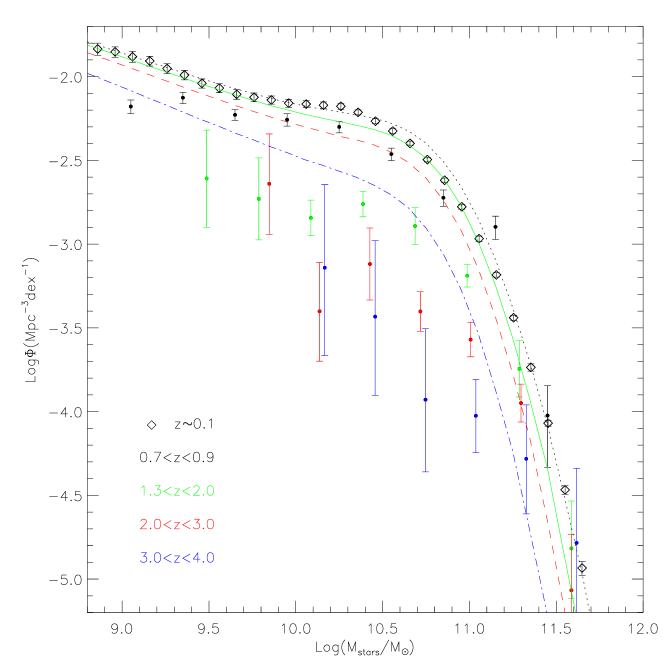
Figure 2: Galaxy stellar mass functions at different redshifts. Symbols with error bars are observational results. Black diomends are SDSS observation of $z\sim 0.1$(Li & White, 2009). Black points are VVDS results in the redshift bin of $[0.7,0.9]$ from Pozzetti et al. (2007). Green, red and blue points are results from Marchesini et al. (2008), in three redshift bins. Lines are model prediction, with black, green, red and blue ones corresponding to results at redshifts of $0.83$, $1.5$, $2.07$ and $3.06$, respectively. Stellar masses of galaxies are normalized to the Chabrier IMF(Chabrier, 2003).

Once we get stellar masses of galaxies at a certain redshift, we can calculate the stellar mass function and also the clustering results at different stellar mass bins at that redshift, combined with the dynamical information of substructures in the simulation. The position of each galaxy is derived directly from Millennium Simulation by following the evolution of substructures. Fig. 1 shows the projected correlation functions at three different stellar mass bins at redshift of around $0.8$. Symbols with error bars are results from VVDS observation(Meneux et al., 2008), and dashed lines are the derived results from our simple model. The projected correlation functions predicted by the model are in reasonably good agreement with the observation from VVDS.

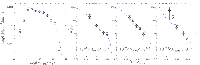
Figure 3: The best-fit model results for fitting both stellar mass function(Pozzetti et al., 2007) and correlation functions in three different stellar mass bins(Meneux et al., 2008) from VVDS observation. Symbols are observational results, and dashed lines are the best fit model results.

Fig. 2 shows the observed stellar mass functions at different redshifts(symbols), compared with the stellar mass functions derived from our model(lines), with the $M_{stars}$-$M_{infall}$ relation taken the same as that of present day. Considering the fact that different initial mass functions(IMF) were adopted in different observations, we convert all stellar masses to the case of the Chabrier IMF(Chabrier, 2003), in this figure and all the figures of stellar mass functions hereafter. The galaxy mass obtained with the Salpeter IMF(Salpeter, 1955) is divided by $1.70$, and that with the Kroupa(Kroupa, 2001) IMF is divided by $1.104$(Cowie & Barger, 2008). It is clear from Fig. 2 that the stellar mass functions are not reproduced under the simple assumption that $M_{stars}$-$M_{infall}$ relation does not evolve with time. Observationally, the number of galaxies with low stellar mass decreases dramatically towards higher redshifts, while the number of high mass galaxies stays roughly unchanged with different redshifts. The model derived results, however, show an opposite trend. The number of low mass galaxies evolves quite slowly, and remains almost the same till redshift $2$, while the number of high mass galaxies evolves a lot, with a much smaller number of galaxies existing at higher redshifts. These results show that the $M_{stars}$-$M_{infall}$ relation must vary at different redshifts. A reasonable model should in general give more massive galaxies and fewer low mass galaxies at higher redshifts than at the local universe. As shown in Fig.3 of Moster et al. (2009), the stellar mass function is more sensitive to the change of model parameters, while the $\chi^{2}$ of correlation functions stays flatter around minimum in a large range of parameter sets. This explains why the correlation functions can be well reproduced while the stellar mass functions show such a large discrepancy. Therefore, correlation function alone is not enough to constrain the $M_{stars}$-$M_{infall}$ relation at $z\sim 0.8$. At the end of this section, we will show that stellar mass function alone is not enough either to give a good constraint on the relation, at least in fitting the current observational data results.

From Fig. 1 and Fig. 2 we know that we need to fit both the stellar mass function and the two point correlation functions to constrain the underlying $M_{stars}$-$M_{infall}$ relation at higher redshifts. Current studies of VVDS observation give both the stellar mass function(Pozzetti et al., 2007) and correlation functions in different stellar mass bins(Meneux et al., 2008) at redshift of $\sim 0.8$. We therefore focus on constraining $M_{stars}$-$M_{infall}$ relation by these VVDS results, building models based on the simulation output at redshift of $0.83$. Following the method of Wang et al. (2006), we assume that the $M_{stars}$-$M_{infall}$ relation at redshift of $\sim 0.8$ can be described by a double power law form. The relation is determined by five parameters for central and satellite galaxies separately, which includes in total 10 parameters in the modelling. When applying the modelling to VVDS results, we notice that compared with the observations of the local Universe, the observational results from higher redshift survey like VVDS provide much fewer data points. Besides, the error bars of these data points are still large, which yields weak constraint on the model. Therefore, on the basis of our previous model of Wang et al. (2006), we alter only the critical mass(and the k parameter simultaneously) when constructing the new model, and keep the rest parameters describing the power law slopes and the relation scatter the same as those for the local Universe of SDSS. In this case, we now have four free parameters that are needed to be constrained.

By fitting both the stellar mass function and the correlation functions of VVDS observation, we get our best-fit model. Stellar mass function is provided by Pozzetti et al. (2007), in the redshift bin of [0.7,0.9], with a mean redshift of $0.81$. The correlation functions are from Meneux et al. (2008), based on the galaxy sample in the redshift range $z=[0.5,1.2]$, with mean redshift of $0.85$. The best fit is defined as the one that makes the ${\Xi}$ minimum.

$${\Xi}=\frac{{\chi}^{2}(\Phi)}{N_{\Phi}}+\frac{{\chi}^{2}_{corr}}{N_{corr}}$$

with

$${{\chi}^{2}(\Phi)}=\sum_{N_{\Phi}}{[\frac{\log{\Phi}-\log{\Phi_{VVDS}}}{\sigma(\log{\Phi_{VVDS}})}]^{2}}$$

and

$${{\chi}^{2}_{corr}}=\sum_{N_{corr}}{[\frac{\log{w(r_{p})}-\log{w(r_{p})_{VVDS}}}{\sigma(\log{w(r_{p})_{VVDS}})}]^{2}}$$

$N_{\Phi}=7$, is the number of points over which the stellar mass function is measured, ranging from $10^{9.5}M_{\odot}$ to $10^{11.6}M_{\odot}$. $N_{corr}=18$, is the number of points over which the correlation function is measured, ranging from $0.2$ to $10.0h^{-1}$Mpc, in three different stellar mass bins.

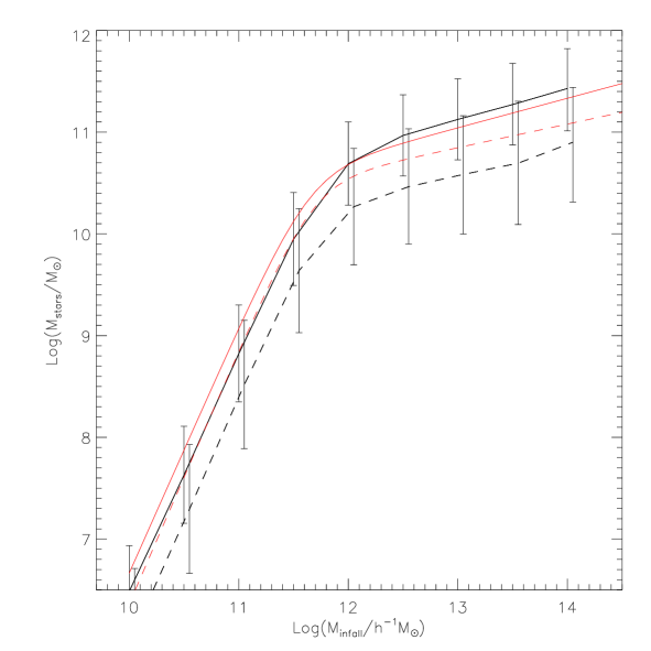
Figure 4: The best-fit $M_{stars}$-$M_{infall}$ relation at $z=0.83$ of central galaxies(black solid line) and satellite galaxies(black dashed line), by fitting both stellar mass function and correlation functions of VVDS observation. For comparison, relations of central(red solid line) and satellite galaxies(red dashed line) from Wang et al. (2006) at $z=0$ are also plotted.

Our best-fit model has the parameters: $M_{0}=6.31\times 10^{11}h^{-1}M_{\odot}$, $\log{k}=10.48$ for central galaxies and $M_{0}=5.03\times 10^{11}h^{-1}M_{\odot}$, $\log{k}=9.99$ for satellite galaxies. The resulting ${\Xi}=3.07591$, with ${\chi}^{2}(\Phi)/N_{\Phi}=1.944$. These parameter values are listed in Tab. 1 to be compared with the best-fit parameters of modelling SDSS observation(Wang et al., 2006). Fig. 3 shows the best-fit model results. Symbols with error bars are the VVDS observation, and dashed lines are the model results. The stellar mass function is well fitted. The clustering is also reasonably reproduced. In Fig. 4, we plot the derived best-fit $M_{stars}$-$M_{infall}$ relation at redshift of $0.83$, for central(black solid line) and satellite(black dashed line) galaxies respectively. In comparison, we over-plotted the relations at redshift $0$ in red lines(solid line for central galaxies and dashed line for satellite galaxies). The result shows that for a given infall mass of hosting halo, the galaxy mass changes with redshift, and the dependence on redshift depends on mass. For massive haloes, the central galaxies inside these haloes are a bit more massive than the galaxies within the same mass of haloes at $z=0$. For less massive haloes, the mass of central galaxies is smaller at higher redshift. For satellite galaxies, however, the mass of galaxies is much smaller toward higher redshift at all mass scales.

Table 1: Best-fit parameter values for the relations between $M_{infall}$ and $M_{stars}$ in different models to fit SDSS and VVDS observations.

		$M_{0}(h^{-1}M_{\odot})$	$\alpha$	$\beta$	$log(k)$	$\sigma$	$\tilde{\chi}^{2}$
SDSS	central	4.0$\times 10^{11}$	0.29	2.42	10.35	0.203	5.010
Wang et al. 2006	satellite	4.32$\times 10^{11}$	0.232	2.49	10.24	0.291
VVDS	central	6.31$\times 10^{11}$	0.29	2.42	10.48	0.203	3.076
this work	satellite	5.03$\times 10^{11}$	0.232	2.49	9.99	0.291
unified model	z=0	3.21$\times 10^{11}$	0.29	2.42	10.17	0.240	6.352
this work	z$\sim 0.8$	4.34$\times 10^{11}$	0.29	2.42	10.15	0.240	8.103

In a recent paper, Moster et al. (2009) claim that stellar mass function alone is enough to constrain the relation between galaxy stellar mass and its hosting halo mass, since the fit to correlation functions has a much wider range at its $\chi^{2}$ minimum than the fit to stellar mass functions. However, this may not be true for higher redshift case. In Fig. 5, we show the derived stellar mass function and correlation functions for the best-fit model when fitting only the stellar mass function of VVDS observation. The results show that the clustering of galaxies is generally over-predicted in this case. Therefore, we believe that fitting both stellar mass function and the correlation functions simultaneously is required to get reasonable fit, at least for the current observational data we can get.

Figure 5: The best-fit model result when fitting only stellar mass function from VVDS observation(Pozzetti et al., 2007). Symbols are observation results, and dashed lines are the best-fit model results.

3 Mass Increase from z$\sim 0.8$ to z$=0$

From high redshift to the present day, dark matter haloes get larger through mergers, and galaxies inside them also become bigger in size. The galaxies gain their masses through either mergers with other galaxies, or by forming new stars. Using the model we build in Sec. 2 we already know the galaxy masses at redshift of $0.83$. We also have galaxy stellar masses of today according to the model built at $z=0$ from Wang et al. (2006). The galaxy mass of today is a total amount of stellar component of galaxy stellar mass that already exists at redshift of $0.83$, the mass increase resulting from mergers with other galaxies, and in addition the newly formed stars during the time interval. By tracing the merger histories of haloes/subhaloes and hence the galaxies that reside in these haloes/subhaloes, the amount of stellar mass that was added through mergers can be calculated. Combined with the stellar mass of galaxies at both $z=0.83$ and $z=0$, the stars that were newly formed during the time interval between these two redshift epochs can be predicted.

For a galaxy that resides in a halo of given mass at $z=0$, we trace back through merger trees to its most massive progenitor at $z=0.83$. We plot in Fig. 6 the median relation between the stellar mass of the most massive progenitor at $z=0.83$ of a galaxy and the mass of its host halo at present day in black solid line. Among the galaxies that merge into this most massive progenitor, some of them are galaxies that already exist at $z=0.83$, including both central and satellite galaxies at that time. The other galaxies are newly formed galaxies after $z=0.83$, and merge into the main group before the present day. From our fitted model results we know that the $M_{stars}$-$M_{infall}$ relation evolves with time. Therefore, at the time of each merger, the mass of the merged galaxy should not be the same as its mass at the time of redshift $0.83$. We get the galaxy mass at the time of each merger by interpolating $M_{stars}$-$M_{infall}$ relation between $z=0.83$ and $z=0$, assuming that the model parameters evolve linearly with redshift.

In Fig. 6, the dotted black line is the sum of the stellar masses at $z=0.83$ of the most massive progenitor and of its satellites merged in. The Red solid line is the result when the merged mass from central galaxies is added, including both the stellar mass existing at $z=0.83$ and those newly formed since then. The contribution from the merged central galaxies is much smaller compared with the mass from merged satellite galaxies. Blue lines are the mass of galaxies of present day, according to our model fit result for SDSS observation(Wang et al., 2006). In the bottom panel of Fig. 6, the corresponding mass ratio of each component to the galaxy of the present day is shown.

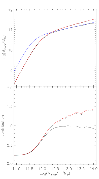
Figure 6: Galaxy mass increase from $z=0.83$ to $z=0$, for different hosting halo masses. Upper panel: for a given mass of haloes at present day, black solid line shows the median value of the most massive progenitors of the central galaxies that reside in them. Dotted black line is the total amount of mass of both the most massive progenitor and the merged galaxies which were satellites at $z=0.83$. Red solid line represents the total mass of the most massive progenitor at $z\sim 0.8$ and all merged galaxies till $z=0$. Blue line is the central galaxy mass of present day, which represents $M_{stars}$-$M_{infall}$ relation at $z=0$. Bottom panel: corresponding ratio of each mass to the galaxy mass of present day.

From Fig. 6 we can tell that for galaxies that reside in haloes of mass less than $10^{12}h^{-1}M_{\odot}$, the mergers since $z=0.83$ contributes to the stellar mass growth by a very small fraction, which can even be ignored. Compared with the galaxy mass at present day, their most massive progenitors contribute from about 20 percent to around 60 percent of the present day mass, while the rest of the mass of $z=0$ galaxies should come from star formation of the central galaxy itself. However, for high mass galaxies whose hosting halo masses are more than $10^{12.5}h^{-1}M_{\odot}$, the story is totally different. The mass of the most massive progenitor galaxy at $z=0.83$ is comparable to its present day mass. When taking into account the stellar component of other merged galaxies, the total mass is significantly larger than the galaxy mass of the present day. This paradoxical result is the consequence of hierarchical merging in the current cosmological model. Here we have adopted the merger trees constructed by de Lucia & Blaizot (2007) for galaxies by taking into account the dynamical time scales. We found that the merged fraction of stellar mass does not change when the merger time scale of Jiang et al. (2008) is adopted. There are several possibilities to reconcile the observations at low and high redshifts in the hierarchical model. One is that satellite galaxies are tidally disrupted in a significant amount of stellar mass before merged into the central galaxies (Yang et al., 2009; Wetzel & White, 2009). However, as we see in §4, the significant tidal disruption is not strongly required by current observational data, because the unified model (details in §4) in which we assume no tidal disruption matches the observational data equally well. Another possibility is that central galaxy mass observationally determined may differ from the galaxy mass defined in simulation, due to the limit size of the observed central region of a galaxy. Besides, when counting for the merged mass in simulation, all stellar masses of the merged galaxies is added, while observationally, the more extended stellar halo around the central galaxy may not be fully counted in. Therefore observationally determined galaxy mass can be smaller than the simulated total mass. With the model advocated here, we expect to study and discriminate these possibilities when the model parameters can be determined better with future high redshift samples of galaxies. Future observations of intra-cluster (group) stars can also help testing these possible mechanisms.

In any case, qualitatively we should be able to conclude that for low mass galaxies, they gain quite a fraction of their present day mass through star formation from $z=0.83$ to today, while for high mass galaxies, most of their present day mass already exist at redshift of $0.83$, and star formation is not active for these galaxies. This is consistent with the result of Wang et al. (2007) where they constrain the star formation histories of galaxies by fitting the spectral distribution properties of galaxies. This is also consistent with the well-known fact that low mass galaxies are in general more active and blue in colour, while high mass galaxies are red and passively evolved.

In Zheng et al. (2007), they use the HOD method to model the luminosity-dependent projected correlation function of DEEP2 and SDSS surveys, and study the stellar mass growth of galaxies, by estimating the stellar mass from galaxy luminosity and colour based on the mean relation between these properties. Compared with their result shown in their Fig.9, the contribution of high redshift galaxies to galaxy mass of the present day has a similar trend with halo mass, but the absolute values of our model are in general higher than their result. Besides, the increase at halo mass of around $10^{12}h^{-1}M_{\odot}$ is more steeper in our model. Notice that they are modelling observation of DEEP2, whose redshift range is around 1, while our model is to fit the VVDS, with redshift of around $0.8$, this discrepancy is in the right direction to be explained by the increase of galaxy mass through time. As pointed out by Zheng et al. (2007), around $25$ percent more of the stellar mass could have been in place in the $z\sim 1$ progenitors due to the fact that the DEEP2 sample they used are not entirely volume limited for red galaxies. This would decrease the discrepancy between these two model results. However, for massive haloes, galaxies inside them are still more massive at higher redshift in our model than in their model result. This may be caused by the fact that the DEEP2 sample could have missed a quite fraction of red massive galaxies because of their colour selection of target galaxies.

4 unified model

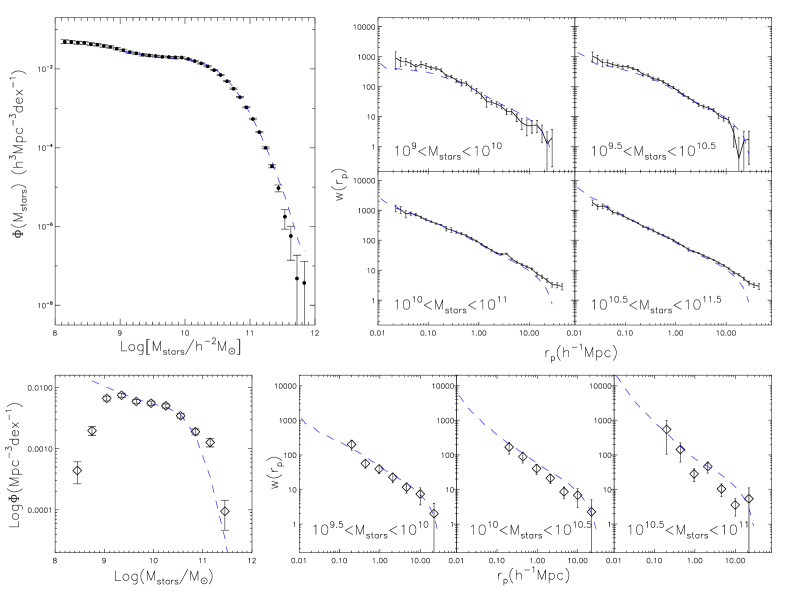
Figure 7: The best-fit unified model results of stellar mass functions and correlation functions at $z=0$(upper panels) and $z=0.83$(lower panels), compared with results from SDSS(Li & White, 2009; Li et al., 2006)(upper panels) and VVDS observation(Pozzetti et al., 2007; Meneux et al., 2008)(lower panels). Symbols with error bars are from observation, and dashed lines are from our best-fit unified model.

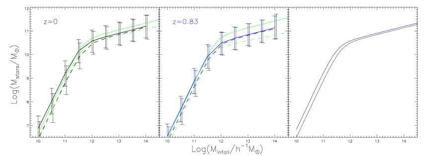
Figure 8: The $M_{stars}$-$M_{infall}$ relation for the best-fit unified model at $z=0$(left panel, black lines) and at $z=0.83$(middle panel, blue lines). Solid lines are the relation for central galaxies and dashed lines are results for satellite galaxies. In the left panel, the $M_{stars}$-$M_{infall}$ relations from the model at $z=0$ of Wang et al. (2006) are over-plotted in solid green lines for central galaxies and dashed green lines for satellite galaxies. In the middle panel, solid and dashed green lines are relations for central and satellite galaxies from our best-fit model in Sec.2 when fitting VVDS observations only. The right panel compares the median relations for central galaxies at $z=0.83$(blue line) and at $z=0$(black line).

When a central galaxy falls into a larger group and becomes a satellite, the gas around the galaxy is shock-heated. The gas stops cooling and the star formation ceases in a short time scale. The stellar mass of the galaxy can increase by only a small amount through star formation. On the other hand, the galaxy stellar mass may decrease a bit due to the tidal stripping effect. We now assume that in total, the stellar components of satellite galaxies do not change compared with the mass at the time when they are central objects. In this case, $M_{stars}$-$M_{infall}$ relation for a satellite galaxy is the same as the $M_{stars}$-$M_{infall}$ relation for centrals at an earlier epoch, when the satellite galaxy falls into a larger group.

We now try to build a unified model to describe the evolution of $M_{stars}$-$M_{infall}$ relation with redshift, for both central and satellite galaxies. We assume that at all redshifts, the median of the $M_{stars}$-$M_{infall}$ relation can be described by a double power law form. We assume that the power law indexes and the scatter around the median relation are fixed with time, while the critical mass and the corresponding normalization parameter evolve with time linearly. At any given redshift, the stellar mass of central galaxy is connected to its host halo mass according to the relation. For satellite galaxy, its stellar mass is connected to its halo mass at infall time, according to the $M_{stars}$-$M_{infall}$ relation at the time when the galaxy falls into a larger group and becomes a satellite.

Based on this picture, we can get the stellar masses for all galaxies at any given redshift, and calculate their stellar mass functions and correlation functions. To get the best fit parameters that describe the evolution relation, we fit at the same time both the observation from SDSS at local Universe(Li & White, 2009; Li et al., 2006), and the VVDS results at redshift of around $0.8$(Pozzetti et al., 2007; Meneux et al., 2008). For simplicity, we fix the slopes describing the $M_{stars}$-$M_{infall}$ relation to be the same as the slopes of the relation of central galaxies when fitting SDSS data only(Wang et al., 2006), i.e., $\alpha=0.29$ and $\beta=2.42$. In total, we now have 5 parameters to fully describe the $M_{stars}$-$M_{infall}$ relation: critical mass $M_{0}$ and $k_{0}$ for redshift 0, $M_{0.8}$, $k_{0.8}$ to describe the relation at $z=0.83$, and the scatter $\sigma$ around the median relation.

The best-fit model is determined when the resulting $\tilde{\Xi}$ gets its minimum.

$${\tilde{\Xi}}=\frac{{\chi}^{2}(\Phi_{0})}{N_{\Phi,SDSS}}+\frac{{\chi}^{2}_{corr,0}}{N_{corr,SDSS}}+\frac{{\chi}^{2}(\Phi_{0.8})}{N_{\Phi,VVDS}}+\frac{{\chi}^{2}_{corr,0.8}}{N_{corr,VVDS}}$$

with

$${{\chi}^{2}(\Phi_{0/0.8})}=\sum_{N_{\Phi,SDSS/VVDS}}{[\frac{\Phi_{0/0.8}-\Phi_{SDSS/VVDS}}{\sigma(\Phi_{SDSS/VVDS})}]^{2}}$$

and

$${{\chi}^{2}_{corr,0/0.8}}=\sum_{N_{corr,0.1/0.8}}{[\frac{w(r_{p})_{0/0.8}-w(r_{p})_{SDSS/VVDS}}{\sigma(w(r_{p})_{SDSS/VVDS})}]^{2}}$$

$N_{\Phi,VVDS}=7$, $N_{\Phi,SDSS}=29$ are the numbers of points over which the stellar mass functions are measured in two observations. $N_{corr,VVDS}=6\times 3$, $N_{corr,SDSS}=30\times 5$, are the numbers of points over which the correlation functions are measured in different stellar mass bins.

Our best-fit model has the parameters: $M_{0}=3.21\times 10^{11}h^{-1}M_{\odot}$, $\log{k_{0}}=10.17$, $M_{0.8}=4.34\times 10^{11}h^{-1}M_{\odot}$, $\log{k_{0.8}}=10.15$, and $\sigma=0.240$. The resulting $\tilde{\Xi}=14.455$, with ${\chi}^{2}(\Phi_{0})/N_{\Phi,SDSS}=3.133$, ${\chi}^{2}_{corr,0}/N_{corr,SDSS}=3.218$, ${\chi}^{2}(\Phi_{0.8})/N_{\Phi,VVDS}=3.778$, and ${\chi}^{2}_{corr,0.8}/N_{corr,VVDS}=4.325$. The parameters are also listed in Table.1. Fig. 7 shows the best-fit model results, compared with the observation from SDSS and VVDS surveys. All the observations are reasonably reproduced, although the resulting ${\chi}^{2}$ is larger, and the fit is a bit poorer than the previous model in Sec.2. The constrained evolution of critical mass $M$ and normalization parameter $k$ can be described as:

$$M(t)=\frac{t_{0}-t}{t_{0}-t_{0.8}}{\times}({M_{0.8}}-{M_{0}})+M_{0}$$

$$k(t)=\frac{t_{0}-t}{t_{0}-t_{0.8}}{\times}({k_{0.8}}-{k_{0}})+k_{0}$$

$t$ is the age of the universe at different redshifts. $t_{0}=13.6098Gyr$, and $t_{0.8}=6.7531Gyr$, are the age of the universe at redshift 0 and $0.83$ respectively.

Fig. 8 shows the best fit $M_{stars}$-$M_{infall}$ relation at two different redshifts. For comparison, we also over-plot the model result when fitting SDSS and VVDS data separately in green lines. We find that at both high and low redshifts, central galaxies in massive haloes are less massive in the unified model than the separate model. The difference of satellite galaxies between the two models is smaller. Although the best-fit $M_{stars}$-$M_{infall}$ relations are different in our two models, they can both give reasonable fits within the observational error range. The main difference of the two models exists for massive galaxies. Considering that the number of high mass galaxies is small in observation, which causes large error bars on the data points, especially for VVDS survey, the statistics of high mass galaxies are not tightly constrained. Therefore different sets of parameters can both give reasonable fits to the observational data. The models can be better constrained only with improved observational data.

In this best-fit unified model, from Fig. 8 we know that both at $z=0$ and $z=0.83$, satellite and central galaxies have similar relation for massive haloes, while for low mass haloes, central galaxies are more massive than satellites. In the most right panel of Fig. 8, we compare the $M_{stars}$-$M_{infall}$ relations for central galaxies at redshift $0$ and $0.83$, for the best-fit unified model results. The evolution of this relation is larger for galaxies in low mass haloes than in more massive haloes. For all masses of haloes, central galaxies that reside in them are more massive at lower redshift than at higher redshift.

Based on the method studying the mass increase of galaxies from redshift of $0.83$ to today described in Sec. 3, we can also detect the mass increase situation according to the result from the unified model stated above. We perform the same analysis as previously stated, and show the results in Fig. 9. We find that the most massive progenitors at $z=0.83$ contribute from around 25 percent at halo mass of $\sim 10^{11}h^{-1}M_{\odot}$ to around 70 percent for haloes massive than $\sim 10^{12.5}h^{-1}M_{\odot}$ to the galaxy mass of present day. This fraction is much smaller for massive galaxies than the separate model. The merged fraction of galaxies, however, is higher in the unified model. Nevertheless, qualitatively the same as in the separate model, the unified model also shows that for galaxies in low mass haloes, they gain their mass from $z=0.83$ to today mainly through star formation, and extra mechanisms are needed to explain the excess of the total progenitor masses to the present-day mass for massive galaxies. Since in the unified model the tidal tripping is assumed to be unimportant, the excess of the stellar mass is presumably located in the stellar haloes of central galaxies. With upcoming larger deep samples of galaxies, we will consider to include the tidal stripping effect in the HOD modeling in a future work.

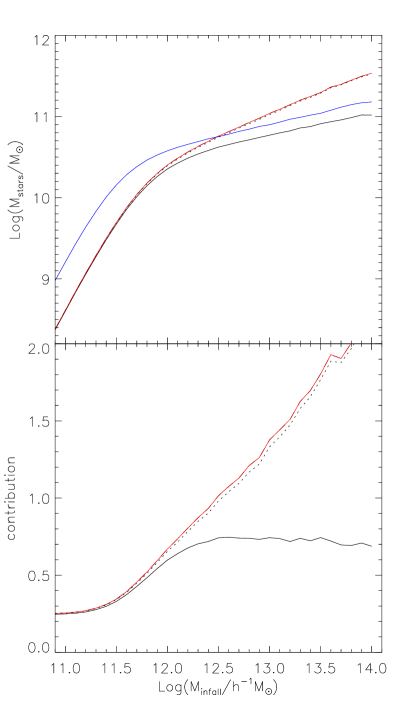
Figure 9: The same as Fig. 6 showing galaxy mass increase from $z=0.83$ to $z=0$ for different host halo masses, except that for the unified model results.

5 Stellar mass functions at higher redshifts

In Sec. 2 and Sec. 4, we build models based on the observations of SDSS and VVDS data of galaxy samples of the local Universe and of redshift of $\sim 0.8$. Assuming that our models can be applied to even earlier epochs, with the parameters evolving linearly with redshift, we can predict stellar mass functions of galaxies at higher redshifts.

Fig. 10 presents the results of stellar mass functions at different redshift bins. Black solid lines are results from recent observation of Kajisawa et al. (2009), for four redshift bins. The stellar masses are normalized to the Chabrier IMF(Chabrier, 2003). The median redshift of $0.5<z<1.0$, $1.0<z<1.5$, $1.5<z<2.5$ and $2.5<z<3.5$ galaxy samples are $0.802$, $1.172$, $2.080$, and $2.952$. In the upper left panel, also plotted is the result of Pozzetti et al. (2007) of VVDS observation in redshift range of $(0.7,0.9)$, which is used in the previous sections to constrain our best-fit models. In the lower two panels, observations from Marchesini et al. (2008) are over-plotted, for $1.3<z<2.0$(green symbols) and $2.0<z<3.0$(red symbols) galaxy samples. Blue dotted and dashed lines are predictions from best-fit models presented in Sec. 2 and Sec. 4, at redshifts of $0.83$, $1.17$, $2.07$, and $3.06$. The results from different observations are consistent with each other, and the predictions from both of our models are also consistent with these observations.

Notice that at all redshifts, the prediction from the unified model gives a higher amplitude of stellar mass function at low mass end, and a lower amplitude at high mass end, compared with the prediction from the model where SDSS and VVDS data are fitted separately. In the unified model, galaxies have smaller masses at high mass end of haloes, and the satellite galaxy mass is higher at high redshift than the separate model. These together cause the difference of amplitudes of stellar mass functions at low and high mass end. As discussed in Sec.4, although the predictions from our two models differ at all redshift bins due to the obvious difference of the $M_{stars}$-$M_{infall}$ relations obtained in the models, it is hard to tell which model is a better description of the real universe observed, due to the poor statistics of current data. Observations with smaller errors will be able to help us build a more precise model.

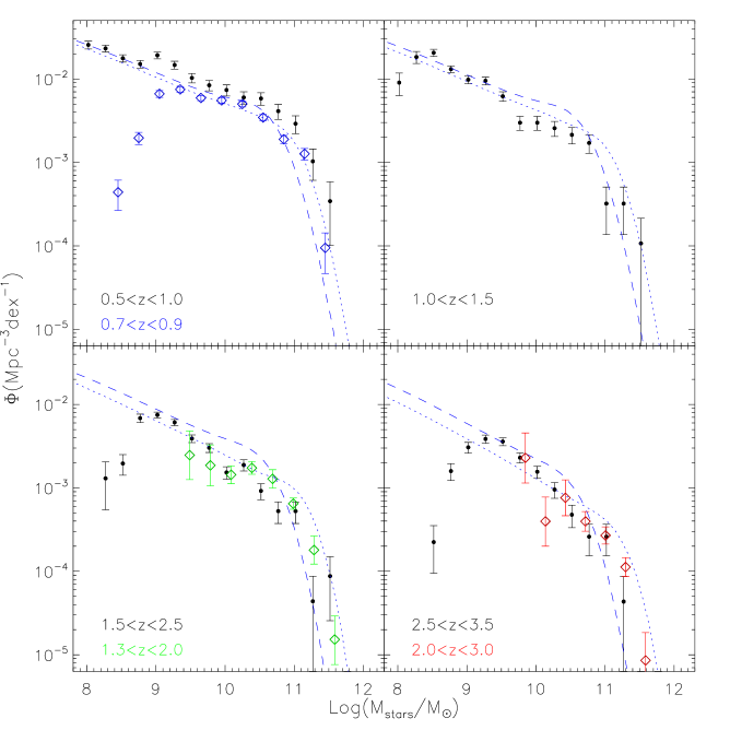
Figure 10: The prediction of stellar mass functions at high redshift of our best-fit models. Black points are observations from Kajisawa et al. (2009), for four redshift bins. Blue dashed lines are the predictions when applying the $M_{stars}$-$M_{infall}$ relation of our unified model to higher redshifts of $0.83$, $1.17$, $2.07$, and $3.06$. Blue dotted lines are predictions of the best-fit models when SDSS and VVDS data are fitted separately, assuming parameters evolve linearly with redshift. In the upper left panel, the observation of Pozzetti et al. (2007) is plotted(blue symbols), for $0.7<z<0.9$ galaxy sample, which is used for building our model at $z0.83$ in Sec. 2. In the lower two panels, observations from Marchesini et al. (2008) are plotted, for $1.3<z<2.0$(green symbols) and $2.0<z<3.0$(red symbols) galaxy samples. Stellar masses of galaxies are normalized to the Chabrier IMF(Chabrier, 2003).

6 Conclusions and discussions

We apply the empirical model of Wang et al. (2006) to higher redshift, to link galaxy stellar mass with its hosting dark matter halo mass at redshift of around $0.8$. The $M_{stars}$-$M_{infall}$ relation is constrained by fitting both the stellar mass function and the correlation functions at different stellar mass intervals from VVDS observation. We find that the difference of $M_{stars}$-$M_{infall}$ relation between central and satellite galaxies at $z\sim 0.8$ are much larger than the galaxies at present day. At all mass scales of haloes, satellite galaxies at $z=0.8$ have much lower stellar masses than satellites within the same mass haloes at $z=0$, while the mass of central galaxies changes less from high redshift to today. Central galaxies are less massive in low mass haloes, and more massive in high mass haloes at $z=0.8$ than the galaxies at $z=0$.

Under the assumption that the mass of satellite galaxy remains about the same as it is a central before it infalls to a larger group, we build a unified model for the $M_{stars}$-$M_{infall}$ relation, which describes the evolution of galaxy mass as a function of halo mass at any given redshift. Satellite stellar mass is determined by the $M_{stars}$-$M_{infall}$ relation of central galaxy at the time of its infall. The best-fit model of both SDSS and VVDS stellar mass functions and clustering functions gives an obvious evolution of $M_{stars}$-$M_{infall}$ relation from $z=0.8$ to $z=0$, with the mass of galaxies at higher redshift being lower than the galaxy mass at the present day, for all masses of hosting haloes. The $M_{stars}$-$M_{infall}$ relation provided by the unified model is different as the relations in the models when SDSS and VVDS data are fitted separately, especially for galaxies with massive haloes and at high redshift. The central galaxies are less massive and satellite galaxies are more massive in the unified model than the separate model. Different sets of parameters can both give reasonable fits to the observed data, because the statistics of high mass galaxies are not tightly constrained in observation at high redshift.

We study the amount of galaxy stellar mass growth from $z\sim 0.8$ to today, in either way of galaxy merger or star formation. For the models when SDSS and VVDS data are fitted separately, we find that for galaxies that reside in haloes of mass less than $10^{12}h^{-1}M_{\odot}$, the masses of their most massive progenitors at $z=0.83$ vary from about 20 percent to 60 percent of the present day mass. Meanwhile, galaxy mergers contribute only a small fraction to the galaxy mass of today. This indicates that a large fraction of $z=0$ stellar masses comes from star formation during the period between $z=0.83$ and $z=0$. For galaxies within massive haloes, the total amount of stellar mass from the main progenitor at $z=0.83$ and from that increased from mergers with other galaxies actually exceeds the present-day galaxy mass. Although there could be a difference of the definitions for stellar mass of central galaxies in observation and in the models based on simulation (for example, the stars in the envelope of the central galaxies may not be counted in observation), this indicates that there may be little star formation ongoing in these massive galaxies. The unified model basically tells the same story, except that the contribution of the most massive progenitors at $z=0.83$ to the mass of the present day is no more than 75 percent even for the most massive galaxies.

Based on the models we build, we give predictions of higher redshift stellar mass functions, with redshift up to $z\sim 3$. It is encouraging that our predictions are consistent with recent observations of stellar mass functions presented by Marchesini et al. (2008) and Kajisawa et al. (2009). However, the amplitude of the stellar mass functions predicted by the unified model is always higher at low mass end, and lower at high mass end, compared with the prediction of the model that fits SDSS and VVDS data separately. Besides, in both of our models, we assume that for the $M_{stars}$-$M_{infall}$ relation, its slopes at high and low mass end and scatter around the median value do not change with time, which may not actually be true. The current models can be tested by future observational data, and a more accurate model can be constructed with better data.

Besides the observational data of VVDS survey used to constrain our model in this work, galaxy stellar mass function and correlation functions in different stellar mass bins are also obtained for zCOSMOS survey by Pozzetti et al. (2009) and Meneux et al. (2009). As pointed out in Meneux et al. (2009), the zCOSMOS field is centred on an extreme overdensity region. We therefore choose to use the VVDS results in this modelling work, although it is possible that the VVDS field is a bit under-dense on the other hand. Hopefully this cosmic variance effect can be significantly reduced with upcoming larger samples of galaxies, based on which the models can be constrained much more tightly.

Recent study of Moster et al. (2009) determined the galaxy stellar mass - halo mass connection at high redshift constrained with stellar mass functions only. They claim that stellar mass function alone is enough to constrain the relation between galaxy stellar mass and their hosting halo mass. We have shown at the end of Sec. 2 that this may not be true for high redshift situation, although this was proved viable when considering models at the local Universe. However, their result shows the same trend as our $M_{stars}$-$M_{infall}$ relation in the separate model, although the quantitatively value of the relation is somewhat different. For low mass haloes, galaxies at higher redshifts have less stellar mass than galaxies at a lower redshift. For high mass haloes, galaxies at high redshift is a bit more massive than galaxies at low redshift. In our unified model, on the other hand, galaxy mass is always smaller at high redshift than that at low redshift, but the difference for galaxies within massive haloes is quite small. The precision of all these models can be tested only by improved observational results both on stellar mass functions and on the clustering properties at high redshifts.

References

- Berlind & Weinberg (2002) Berlind A. A., Weinberg D. H., 2002, ApJ, 575, 587
- Bouwens et al. (2008) Bouwens R. J., Illingworth G. D., Franx M., Ford H., 2008, ApJ, 686, 230
- Bower et al. (2006) Bower R. G., Benson A. J., Malbon R., Helly J. C., Frenk C. S., Baugh C. M., Cole S., Lacey C. G., 2006, MNRAS, 370, 645
- Bullock et al. (2002) Bullock J. S., Wechsler R. H., Somerville R. S., 2002, MNRAS, 329, 246
- Chabrier (2003) Chabrier G., 2003, PASP, 115, 763
- Coil et al. (2006) Coil A. L., Newman J. A., Cooper M. C., Davis M., Faber S. M., Koo D. C., Willmer C. N. A., 2006, ApJ, 644, 671
- Conroy et al. (2006) Conroy C., Wechsler R. H., Kravtsov A. V., 2006, ApJ, 647, 201
- Cooray (2005) Cooray A., 2005, MNRAS, 364, 303
- Cooray & Ouchi (2006) Cooray A., Ouchi M., 2006, MNRAS, 369, 1869
- Cowie & Barger (2008) Cowie L. L., Barger A. J., 2008, ApJ, 686, 72
- Davis et al. (2003) Davis M., Faber S. M., Newman J., Phillips A. C., Ellis R. S., Steidel C. C., Conselice C., Coil A. L., et al., 2003, in Guhathakurta P., ed., Society of Photo-Optical Instrumentation Engineers (SPIE) Conference Series Vol. 4834 of Society of Photo-Optical Instrumentation Engineers (SPIE) Conference Series, Science Objectives and Early Results of the DEEP2 Redshift Survey. pp 161–172
- de Lucia & Blaizot (2007) de Lucia G., Blaizot J., 2007, MNRAS, 375, 2
- Drory et al. (2004) Drory N., Bender R., Feulner G., Hopp U., Maraston C., Snigula J., Hill G. J., 2004, ApJ, 608, 742
- Drory et al. (2005) Drory N., Salvato M., Gabasch A., Bender R., Hopp U., Feulner G., Pannella M., 2005, ApJ, 619, L131
- Elsner et al. (2008) Elsner F., Feulner G., Hopp U., 2008, A&A, 477, 503
- Erickson et al. (1987) Erickson L. K., Gottesman S. T., Hunter Jr. J. H., 1987, Nature, 325, 779
- Fontana et al. (2006) Fontana A., Salimbeni S., Grazian A., Giallongo E., Pentericci L., Nonino M., Fontanot F., Menci N., Monaco P., Cristiani S., Vanzella E., de Santis C., Gallozzi S., 2006, A&A, 459, 745
- Jiang et al. (2008) Jiang C. Y., Jing Y. P., Faltenbacher A., Lin W. P., Li C., 2008, ApJ, 675, 1095
- Jing et al. (1998) Jing Y. P., Mo H. J., Boerner G., 1998, ApJ, 494, 1
- Kajisawa et al. (2009) Kajisawa M., Ichikawa T., Tanaka I., Konishi M., Yamada T., Akiyama M., Suzuki R., Tokoku C., Uchimoto Y. K., Yoshikawa T., Ouchi M., Iwata I., Hamana T., Onodera M., 2009, ArXiv e-prints
- Kravtsov et al. (2004) Kravtsov A. V., Berlind A. A., Wechsler R. H., Klypin A. A., Gottlöber S., Allgood B., Primack J. R., 2004, ApJ, 609, 35
- Kroupa (2001) Kroupa P., 2001, MNRAS, 322, 231
- Le Fèvre et al. (2005) Le Fèvre O., Vettolani G., Garilli B., Tresse L., Bottini D., Le Brun V., Maccagni D., Picat J. P., et al., 2005, A&A, 439, 845
- Li et al. (2006) Li C., Kauffmann G., Jing Y. P., White S. D. M., Börner G., Cheng F. Z., 2006, MNRAS, 368, 21
- Li & White (2009) Li C., White S. D. M., 2009, ArXiv e-prints
- Lilly et al. (2009) Lilly S. J., LeBrun V., Maier C., Mainieri V., Mignoli M., Scodeggio M., Zamorani G., Carollo M., et al., 2009, ApJS, 184, 218
- Mandelbaum et al. (2006) Mandelbaum R., Seljak U., Kauffmann G., Hirata C. M., Brinkmann J., 2006, MNRAS, 368, 715
- Mandelbaum et al. (2005) Mandelbaum R., Tasitsiomi A., Seljak U., Kravtsov A. V., Wechsler R. H., 2005, MNRAS, 362, 1451
- Marchesini et al. (2008) Marchesini D., van Dokkum P. G., Forster Schreiber N. M., Franx M., Labbe’ I., Wuyts S., 2008, ArXiv e-prints
- Meneux et al. (2009) Meneux B., Guzzo L., de la Torre S., Porciani C., Zamorani G., Abbas U., Bolzonella M., Garilli B., et al., 2009, ArXiv e-prints
- Meneux et al. (2008) Meneux B., Guzzo L., Garilli B., Le Fèvre O., Pollo A., Blaizot J., De Lucia G., Bolzonella M., et al., 2008, A&A, 478, 299
- Moster et al. (2009) Moster B. P., Somerville R. S., Maulbetsch C., van den Bosch F. C., Maccio’ A. V., Naab T., Oser L., 2009, ArXiv e-prints
- Pollo et al. (2006) Pollo A., Guzzo L., Le Fèvre O., Meneux B., Cappi A., Franzetti P., Iovino A., McCracken H. J., et al., 2006, A&A, 451, 409
- Pozzetti et al. (2007) Pozzetti L., Bolzonella M., Lamareille F., Zamorani G., Franzetti P., Le Fèvre O., Iovino A., Temporin S., et al., 2007, A&A, 474, 443
- Pozzetti et al. (2009) Pozzetti L., Bolzonella M., Zucca E., Zamorani G., Lilly S., Renzini A., Moresco M., Mignoli M., et al., 2009, ArXiv e-prints
- Reddy et al. (2008) Reddy N. A., Steidel C. C., Pettini M., Adelberger K. L., Shapley A. E., Erb D. K., Dickinson M., 2008, ApJS, 175, 48
- Salpeter (1955) Salpeter E. E., 1955, ApJ, 121, 161
- Scoville et al. (2007) Scoville N., Aussel H., Brusa M., Capak P., Carollo C. M., Elvis M., Giavalisco M., Guzzo L., et al., 2007, ApJS, 172, 1
- Springel et al. (2005) Springel V., White S. D. M., Jenkins A., Frenk C. S., Yoshida N., Gao L., Navarro J., Thacker R., et al., 2005, Nature, 435, 629
- Vale & Ostriker (2004) Vale A., Ostriker J. P., 2004, MNRAS, 353, 189
- van den Bosch et al. (2003) van den Bosch F. C., Yang X., Mo H. J., 2003, MNRAS, 340, 771
- Wang et al. (2006) Wang L., Li C., Kauffmann G., de Lucia G., 2006, MNRAS, 371, 537
- Wang et al. (2007) Wang L., Li C., Kauffmann G., De Lucia G., 2007, MNRAS, 377, 1419
- Wetzel & White (2009) Wetzel A. R., White M., 2009, ArXiv e-prints
- White et al. (2007) White M., Zheng Z., Brown M. J. I., Dey A., Jannuzi B. T., 2007, ApJ, 655, L69
- Wolf et al. (2004) Wolf C., Meisenheimer K., Kleinheinrich M., Borch A., Dye S., Gray M., Wisotzki L., Bell E. F., Rix H.-W., Cimatti A., Hasinger G., Szokoly G., 2004, A&A, 421, 913
- Yan et al. (2003) Yan R., Madgwick D. S., White M., 2003, ApJ, 598, 848
- Yang et al. (2003) Yang X., Mo H. J., van den Bosch F. C., 2003, MNRAS, 339, 1057
- Yang et al. (2009) Yang X., Mo H. J., van den Bosch F. C., 2009, ApJ, 693, 830
- Zehavi et al. (2005) Zehavi I., Zheng Z., Weinberg D. H., Frieman J. A., Berlind A. A., Blanton M. R., Scoccimarro R., Sheth R. K., et al., 2005, ApJ, 630, 1
- Zheng (2004) Zheng Z., 2004, ApJ, 610, 61
- Zheng et al. (2007) Zheng Z., Coil A. L., Zehavi I., 2007, ApJ, 667, 760