Antiferromagnetism of Repulsively Interacting Fermions in a harmonic trap

Abstract

We propose a Real-Space Gutzwiller variational approach and apply it to a system of repulsively interacting ultracold fermions with spin $\frac{1}{2}$ trapped in an optical lattice with a harmonic confinement. Using the Real-Space Gutzwiller variational approach, we find that in system with balanced spin-mixtures on a square lattice, antiferromagnetism either appears in a checkerboard pattern or forms a ring and antiferromagnetic order is stable in the regions where the particle density is close to one, which is consistent with the recent results obtained by the Real-Space Dynamical Mean-field Theory approach. We also investigate the imbalanced case and find that antiferromagnetic order is suppressed there.

I Introduction

Ultracold atomic gases have attracted much attention ATOM_1 since the first realization of Bose-Einstein condensation ATOM_2 . In recent years, ultracold atoms in optical lattices have stimulated a new wave of studying the many-body problems. One can obtain optical lattices by confining the ultracold atoms in periodic trapping potentials created with counter-propagating laser beams OPT_1 . Owing to the large degree of control over the optical lattice parameters such as the geometry and depth of the potential, optical lattices provide an ideal playground for studying fundamental condensed-matter physics problems. Many remarkable phenomena, like the quantum phase transition from a superfluid to a Mott-insulator in a Bose-Einstein condensate with repulsive interaction OPT_2 and the superexchange interactions with ultracold atoms OPT_3 have been observed experimentally in optical lattices. In addition, loading ultracold fermions as well as mixtures of bosonic and fermionic quantum gases in optical lattices has also become a topic of intensive study OPT_4 ; OPT_5 ; OPT_6 .

Although optical lattices have been providing an ideal stage for both theoretical and experimental studies of fundamental problems in condensed matter physics, when compared to true solid state system, defects arise. For example, in optical lattices, an additional harmonic confinement is always present due to the gaussian profile of the laser beams OPT_1 . Although this harmonic confinement is usually weak and varies slowly (typically around 10-200 Hz oscillation frequencies) compared to the confinement of the atoms on each lattice site (typically around 10-40 kHz), it generally leads to an inhomogeneous environment for the trapped atoms. Therefore, in order to make problems more relevant to condensed matter systems, investigating how the harmonic confinement affects the behavior of atoms trapped in optical lattices is important. Motivated by this, we take the ultracold fermions with spin $\frac{1}{2}$ into consideration and concentrate on the magnetic behavior of these particles in such a harmonic confinement.

For simplicity, in this paper we consider the square lattice with a single orbital per site as a model, which can be described by the famous Hubbard Hamiltonian. Hubbard model has been studied by various methods such as variational Monte-Carlo method VMC and dynamical mean-filed theory DMFT . Here we apply the Gutzwiller approximation GV_5 , which was introduced by Gutzwiller along with his proposal of Gutzwiller wave function (GWF). It turns out that Gutzwiller approximation is exact in the limit of infinite dimensions. Extensions to multi-band correlated systems using Gutzwiller approximation were carried out by J. Bünemann et al. GV_6 . Meanwhile, Gutzwiller approximation was proved to be equivalent to slave-boson theories SLBT_1 ; SLBT_2 ; SLBT_3 on a mean-field level for both one-band case SLBT_4 and multi-band case SLBT_5 ; SLBT_6 . Gutzwiller approximation is usually used in homogenous environment, here we extends it to inhomogeneous environment and address the problem in real space. The organization of the paper is as follows: first, we introduce the Hubbard Hamiltonian as well as the Gutzwiller variational approach (GVA). Then we show how the harmonic confinement potential and the repulsive interaction affect the magnetism of the system in the case of balanced spin-mixtures and then we present the results obtained in a imbalanced case. Finally, we make some discussions and conclusions.

II Model and Method

We apply the Hubbard model for repulsively interacting fermions in an optical lattice. The Hamiltonian is described as

$$H = H_{0}+H_{int}$$

$$H_{0} = -\sum_{\langle ij\rangle,\sigma}t_{ij}c_{i\sigma}^{\dagger}c_{j\sigma}$$

$$H_{int} = U\sum_{i}n_{i\uparrow}n_{i\downarrow}+\sum_{i\sigma}(V_{i}-\mu)n_{i\sigma}$$ (1)

where $n_{i\sigma}=c^{\dagger}_{i\sigma}c_{i\sigma}$, and $c_{i\sigma}(c^{\dagger}_{i\sigma}$) are fermionic annihilation (creation) operators for an atom at the $i$th site with spin $\sigma$. $t_{ij}$ describes the hopping amplitude between nearest neighbor sites $\langle ij\rangle$. If $i$ and $j$ are nearest neighbors, $t_{ij}=t$, otherwise, $t_{ij}=0$. $U>0$ is the repulsive interaction, $\mu_{\sigma}$ is the chemical potential and $V_{i}=\frac{1}{2}\Omega^{2}r_{i}^{2}=V_{0}r_{i}^{2}$ is the external trapping potential, in which $r_{i}$ is the distance measured from the center of the system. As pointed out in reference OPT_1 , $\Omega$ is usually much smaller than the characteristic frequency of the optical lattice, providing a spatially slowly varying chemical potential.

Many methods, such as Hartree-Fock theory HF and Real-Space Dynamical Mean-Field Theory (R-DMFT) approach RDMFT , have been used to study the ground state of Hubbard model with a confinement potential. Among these methods, R-DMFT approach is the most accurate and reliable one, because it includes all the local quantum fluctuation. However, the solution of Anderson impurity model in each iteration step makes it very time-consuming. Here we apply the Real-Space Gutzwiller variational approach (R-GVA) for this model. We will show that the results obtained by R-GVA is consistent with those obtained by R-DMFT approach.

The GVA has been proved to be quite efficient and accurate GV_1 ; GV_2 ; GV_3 for the ground state studies of many important phenomena in strongly correlated system, i.e. the Mott transition, ferromagnetism and superconductivityqianghua ; qianghua2 . It has also been demonstrated GV_4 that GVA is as accurate as DMFT method for the ground state properties, but much computationally cheaper, which grants this approach much validity.

We first give a description of GVA for the ground state of correlated electron model systems. There are $2$ different spins and each of them could be either empty or occupied, thus totally we have $2^{2}=4$ number of local configurations $|\Gamma\rangle$ on a single site. Those possible configurations should not be equally weighted, because electrons tend to occupy configurations which have relatively lower energy. For this purpose, we could construct projectors which can reduce the specified high energy configurations $|\Gamma\rangle$ on site $i$

$$\hat{m}_{i\Gamma}=\left|{i,\Gamma}\right\rangle\left\langle{i,\Gamma}\right|$$ (2)

which fufills,

$$\sum_{\Gamma}\hat{m}_{i\Gamma}=1$$ (3)

since all the configurations ${|\Gamma\rangle}$ form a locally complete set of basis.

In Eq.(II), if the interactions are absent, the ground state is exactly given by the Hartree uncorrelated wave function (HWF) $|\Psi_{0}\rangle$, which is a single determinant of single particle wave functions. However, after turning on the interaction terms, the HWF is no-longer a good approximation, since it contains many energetically unfavorable configurations. In order to describe the ground state better, the weights of those unfavorable configurations should be suppressed. This is the main spirit of Gutzwiller wave function (GWF). GWF $|\Psi_{G}\rangle$ is constructed by acting a many-particle projection operator on the uncorrelated HWF,

$$|\Psi_{G}\rangle=\mathcal{\hat{P}}|\Psi_{0}\rangle$$

$$\mathcal{\hat{P}} =\prod\limits_{i}\hat{P}_{i}=\prod\limits_{i}\sum_{\Gamma}\lambda_{i\Gamma}\hat{m}_{i\Gamma}$$ (4)

The projection operator $\mathcal{\hat{P}}$ is used to adjust the weight of site configurations through parameters $\lambda_{i\Gamma}$ ($0\leq\lambda_{i\Gamma}\leq 1$). The GWF falls back to uncorrelated HWF if all $\lambda_{i\Gamma}=1$. On the other hand, if $\lambda_{i\Gamma}=0$, the configuration $\Gamma$ of site $i$ will be totally removed. In this way, both the itinerant behavior of uncorrelated wave functions and localized behavior of atomic configurations can be described consistently, and the GWF will give a more reasonable physical picture of correlated systems than HWF does.

The evaluation of GWF is a difficult task due to its multi-configuration nature. There are lots of efforts in the literature, and the most famous one is Gutzwiller approximation GV_5 . In this approximation, the inter-site correlation effect has been neglected and the physics meaning was discussed in GV_1 and GV_7 . The exact evaluation of the single-band GWF in one dimension one_dim and in the limit of infinite dimensions in_dim were carried out. It turns out that Gutzwiller approximation is exact in the latter case.

The expectation value of Hamiltonian Eq.(1) is:

$$\langle H\rangle_{G}=\frac{\langle\Psi_{G}|H|\Psi_{G}\rangle}{\langle\Psi_{G}|\Psi_{G}\rangle}=\frac{\langle\Psi_{0}|\mathcal{\hat{P}}H\mathcal{\hat{P}}|\Psi_{0}\rangle}{\langle\Psi_{0}|\mathcal{\hat{P}}^{2}|\Psi_{0}\rangle}$$ (5)

We note that by choosing $\lambda_{i\Gamma}=\sqrt{\frac{m_{i\Gamma}}{m_{i\Gamma}^{0}}}$, $|\Psi_{G}\rangle$ is normalized under GA. $\langle\Psi_{G}|\Psi_{G}\rangle=\prod\limits_{i}\langle\Psi_{0}|\hat{P}_{i}^{2}|\Psi_{0}\rangle=\prod\limits_{i}\sum_{\Gamma}\frac{m_{i\Gamma}}{m_{i\Gamma}^{0}}\langle\Psi_{0}|\hat{m}_{i;\Gamma}|\Psi_{0}\rangle=\prod\limits_{i}\left(\sum_{\Gamma}m_{i\Gamma}\right)=1$. Here $m_{i\Gamma}$ is the weight of configuration $\Gamma_{i}$, $m_{i\Gamma}=\langle\Psi_{G}|\hat{m}_{i\Gamma}|\Psi_{G}\rangle$ and $m_{i\Gamma}^{0}=\langle\Psi_{0}|\hat{m}_{i\Gamma}|\Psi_{0}\rangle$. In the first equality we separate the average of a projection operator string into the product of single site averages.

The expectation value of kinetic energy is

$$\langle\Psi_{G}|H_{0}|\Psi_{G}\rangle$$

$$= \sum_{i,j,\sigma}z_{i\sigma}z_{j\sigma}t_{ij}\langle\Psi_{0}|c_{i\sigma}^{\dagger}c_{j\sigma}|\Psi_{0}\rangle$$ (6)

where

$$z_{i\sigma}=\sum_{\Gamma_{i},\Gamma_{i}^{\prime}}\frac{\sqrt{m_{\Gamma_{i}}m_{\Gamma_{i}^{\prime}}}D_{\Gamma_{i}^{\prime}\Gamma_{i}}^{\sigma}}{\sqrt{n_{i\sigma}^{0}\left(1-n_{i\sigma}^{0}\right)}}$$ (7)

with $D_{\Gamma^{\prime}\Gamma}^{\sigma}=|<\Gamma^{\prime}|c_{i\sigma}^{\dagger}|\Gamma>|$, $0\leq z_{i\sigma}\leq 1$.

while for the interaction part of the Hamiltonian

$$\langle\Psi_{G}|H_{int}|\Psi_{G}\rangle$$

$$=\sum_{i}\sum_{\Gamma}E_{\Gamma}\frac{m_{i\Gamma}}{m_{i\Gamma}^{0}}\langle\Psi_{0}|\hat{m}_{i\Gamma}|\Psi_{0}\rangle$$

$$=\sum_{i}\sum_{\Gamma}E_{\Gamma}m_{i\Gamma}$$ (8)

Putting Eq.(6) and Eq.(8) together, we have the following equation for the limit of infinite dimensions

$$\langle H\rangle_{G}$$

$$=\sum_{i\neq j,\sigma}t_{i,j}z_{i,\sigma}z_{j,\sigma}\langle c_{i\sigma}^{\dagger}c_{j\sigma}\rangle_{0}+\sum_{i,\sigma}\epsilon_{i\sigma}n_{i,\sigma}^{0}+\sum_{i,\Gamma}E_{i\Gamma}m_{i\Gamma}$$

$$=\langle 0|H_{eff}|0\rangle$$ (9)

In an inhomogeneous systems, the spatial dependence of $z_{i\sigma}$ is preserved and the variation is in the $4N_{s}$ parameter space, where $N_{s}$ is the number of sites. We adopt the following algorithm to minimize $\langle H\rangle_{G}$. We begin with solving $H_{eff}$ where the $Z$-factors are fixed, from which we compute the expectation value of the Fermionic operators on the ground state. Then the minimization of the Gutzwiller variational parameter $m$ is done in the alternating least squares (ALS) scheme, in which we fix the $m_{\Gamma}$s on all but the current site and the problem reduces to quadratic optimization which is solved as an eigen-problem. Using Eq.(7), one could compute the $Z$-factor on each site, and then they are plugged into the non-interacting model $H_{eff}$ as parameters. The iteration is finished when the difference of $Z$-factors from two step is less then the given precision, say $10^{-6}$. In general, there is no guarantee that the ALS method will converge to the global optimum and the convergence of the iteration. However, in practice, this does not seem to occur as long as one varies the parameters in the Hamiltonian adiabatically.

In the following part, we consider this model on a $(24\times 24)$ square lattice at half filling (one particle per site) and set $t$ as the unit of energy.

III Results and Discussions

Now we present the numerical results obtained with the R-GVA. We focus on the spatial dependence of magnetization and particle distribution at different parameters. We first consider the balanced situation in which the number of spin-$\uparrow$ particles is the same to that of the spin-$\downarrow$ ones. We begin with the discussion on the effect of the harmonic confinement $V$. First we fix the repulsive interaction $U=5$. The spatial distribution of magnetization at different strengths of $V$ is shown in Fig. 1.

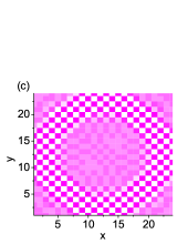
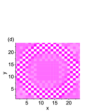
Figure 1: (Color online) Real-Space magnetization profiles for $U=5$ on square lattice $(24\times 24)$ at half filling, when (a) $V=0.01$, (b) $V=0.02$, (c) $V=0.03$, (d) $V=0.04$. AF region shrinks as the confining potential increases.

We find that antiferromagnetic(AF) order exists even with the presence of the inhomogeneous harmonic confinement. It is seen clearly from Fig. 1 that how the pattern of magnetization evolves as the harmonic confinement $V$ increases. As the confinement potential $V$ is enhanced, the antiferromagnetism changes from a uniform checkerboard structure to a ring, where the filling is close to $1$.

To make the problem more explicit, we also get the particle and spin density profiles along x-direction. In Fig. 2 (a) and (b), we present the local density $\langle n\rangle_{i}$ and the absolute value of the staggered magnetism $\langle m_{i}\rangle$ as the function of the distance along $y=12$, where $\langle n_{i}\rangle=\langle n_{i\uparrow}\rangle+\langle n_{i\downarrow}\rangle$ and $\langle m_{i}\rangle=\frac{1}{2}(\langle n_{i\uparrow}\rangle-\langle n_{i\downarrow\rangle})$. We find that in the presence of the confinement potential $V$, the antiferromagnetic phase is stable when the local density is close to $1$, which is consistent with the result obtained in reference RDMFT . The results obtained here confirm the role that the harmonic confinement plays in affecting the antiferromagnetic pattern among the fermions in optical lattices. As pointed out in RDMFT , these results are important for the ongoing attempt to realize antiferromagnetic state of fermions with repulsive interactions in periodic potentials.

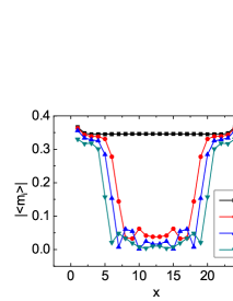
Figure 2: (Color online) Particle density and the absolute value of staggered magnetization as the function of the distance along $y=12$ for $U=5$ at different confining potentials at half filling: (a) the density profile; (b) the staggered magnetization.

Next, we concentrate on the effect of the repulsive interaction $U$. Experimentally, $U$ could be tuned by the Feshbach resonance technique. We first set the confining potential $V$ as 0.02. The spatial dependence of magnetization and the local particle distribution for at different strengths of $U$ are presented in Fig. 3 and Fig. 4. We know that the ground state of ultra-cold fermions loading in an optical lattice without trap follows the spin density wave (SDW) mean filed prediction at weak coupling. Approaching the strong coupling limit, the large repulsive interaction drives the system to an AF insulator phase. From Fig. 3 and Fig. 4, we can see that the confining potential $V$ plays a dominant role at weak coupling and the SDW state is suppressed, while at strong coupling, the repulsive interaction $U$ plays a dominant role and the AF order is stable.

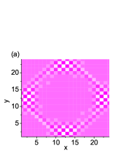
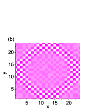
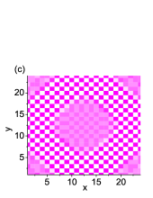
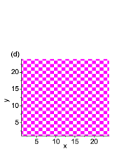
Figure 3: (Color online) Real-Space magnetization profiles for $V=0.02$ on square lattice $(24\times 24)$ at half filling, when (a) $U=2$, (b) $U=3$, (c) $U=5$, (d) $U=9$. The Af region expands as $U$ increases.

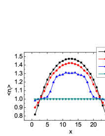
Figure 4: (Color online) Particle density profile along $y=12$ for $V=0.02$ at different strengths of repulsive interaction $U$ at half filling. The particle density is more and more close to $1$ as $U$ increases.

We now investigate the case of imbalanced spin-mixtures, i.e. when $N_{\uparrow}\not=N_{\downarrow}$. The spatial dependence of magnetism and the particle density of sublattice at different strengths of imbalance are presented in Fig. 5 and Fig. 6. We find that as the imbalance is enhanced, the AF order decreases. In balanced system, antiferromagnetism competes with the confining potential $V$. Upon imbalanced spin-mixtures, it follows that an equivalent magnetic field is added into the system, therefore the AF order is destroyed.

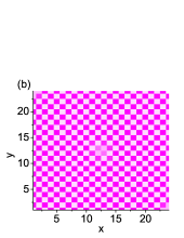
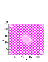
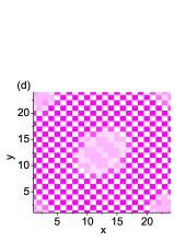
Figure 5: (Color online) Real-Space magnetization profiles for $V=0.01$ and $U=5$ on square lattice $(24\times 24)$ for imbalanced spin-mixtures at half filling, when (a) $N_{\downarrow}=288,N_{\uparrow}=288$; (b) $N_{\downarrow}=286,N_{\uparrow}=290$; (c) $N_{\downarrow}=275,N_{\uparrow}=301$; (d) $N_{\downarrow}=270,N_{\uparrow}=306$. The AF order decreases as the imbalance is enhanced.

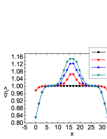
Figure 6: (Color online) Particle density profile as the function of the distance along $y=x$ for $U=5$ and $V=0.01$ for different spin-mixtures at half filling. The particle density in the center of the system increases as the imbalance is enhanced.

IV Experimental Signatures

Spatial distribution of spin density in a harmonic trap predicted in this paper could be detected by Bragg scattering MET_1 , and by spatial microwave transition and spin-changing collisions techniques, which measure the integrated density profiles along chosen directions MET_2 .

V Conclusion

In conclusion, we have developed the fast Real-Space Gutzwiller variational approach which is suitable for the fast determination of the grounds state phase diagram of the inhomogeneous strongly correlated systems. With this method, we have studied both balanced and imbalanced case of fermions with spin $\frac{1}{2}$ trapped in an optical lattice with a harmonic confinement potential. We find that the trap potential tends to destroy the AF order in the center as well as the edge of the trap, leaving a ring of AF region with local density close to $1$. The AF order is suppressed for imbalanced system. These results are meaningful for the ongoing attempt to realize AF in the optical lattices. We anticipate that this R-GVA scheme could also be applied to other systems, such as a strongly interacting Bose-Fermi mixture in a harmonic trap.

References

- (1) For a review, see Nature (London) 416, (2002) 205-246.
- (2) M. H. Anderson, J. R. Ensher, M. R. Matthews, C. E. Wieman, and E. A. Cornell, Science 269, (1995) 198.
- (3) I. Bloch, Nature Physics 1, (2005) 23
- (4) M. Greiner, O. Mandel, T. Esslinger, T. W. Hansch, and I. Bloch, Nature (London) 415, 39 (2002)
- (5) S. Trotzky, P. Cheinet, S. Flling, M. Feld, U. Schnorrberger, A. N. Rey, A. Polkounikov, E. A. Demler, M. D. Lukin, I. Bloch, Science 319, 295 (2008)
- (6) J. K. Chin et al, Nature 443, 961 (2006)
- (7) A. Albus, F. Illuminati, J. Eisert, Phys. Rev. A 68, 023606 (2003)
- (8) R. Roth, K. Burnett, Phys. Rev. A 69, 021601(R) (2004)
- (9) Hisatoshi Yokoyama and Hiroyuki Shiba, J. Phys. Soc. Jpn. 56 (1987) pp. 1490-1506
- (10) K. Held, M. Ulmke, N. Blmer, and D. Vollhardt, Phys. Rev. B 56, 14469 (1997)
- (11) M. C. Gutzwiller, Phys. Rev. Lett. 10, 159 (1963); M. C. Gutzwiller, Phys. Rev. 134, A923 (1964); M. C. Gutzwiller, Phys. Rev. 137, A1726 (1965).
- (12) J. Bünemann, F. Gebhard, and W. Weber, J. Phys: Cond-Matt, 9, 7343 (1997); J. Bünemann, and W. Weber, Phys. Rev. B 55, 4011 (1997); J. Bünemann, and W. Weber, F. Gebhard, Phys. Rev. B 57, 6896 (1998); J. Bünemann, F. Gebhard, and W. Weber, Foundations of Physics 30, 2011 (2000); C. Attaccalite and M. Fabrizio, Phys. Rev. B 68, 155117 (2003).
- (13) G. Kotliar and A. E. Ruckenstein, Phys. Rev. Lett. 57, 1362 (1986)
- (14) P. Coleman, Phys. Rev. B 28, 5255 (1983); 29, 3035 (1984); 35, 5072 1987; N. Read and D. M. Newns, J. Phys. C 16, 3273 1983; Adv. Phys. 36, 799 1987.
- (15) F. Lechermann, A. Georges, G. Kotliar, and O. Parcollet, Phys. Rev. B 76, 155102 (2007)
- (16) F. Gebhard, The Mott Metal-Insulator Transition-Models and Methods, Springer Tracts in Modern Physics Vol. 137 (Springer, Berlin, 1997)
- (17) F. Gebhard, Phys. Rev. B 44, 992 (1991).
- (18) J. Bünemann, F. Gebhard, and W. Weber, Phys. Rev. B 76, 193104 (2007)
- (19) T. Gottwald and P. G. J. van Dongen, Phys. Rev. A 80, 033603 (2009).
- (20) M. Snoek, I. Titvinidze, C. Tke, K. Byczuk, and W. Hofstetter, New J. Phys. 10, 093008 (2008).
- (21) W. F. Brinkman, T. M. Rice, Phys. Rev. B 2, 4302 (1970)
- (22) F. C. Zhang, C. Gros, T. M. Rice, H. Shiba, Supercond. Sci. Technol. 1, 36 (1988).
- (23) D. Vollhardt, Rev. Mod. Phys. 56, 99 (1984)
- (24) Qiang-Hua Wang, Z. D. Wang, Y. Chen and Fu-Chun Zhang, Phys. Rev. B 73, 092507 (2006).
- (25) Jung Hoon Han, Qiang-Hua Wang, and Dung-Hai Lee, Int. J. Mod. Phys. B 15, 1117 (2001).
- (26) XiaoYu Deng, Lei Wang, Xi Dai, Zhong Fang, Phys. Rev. B 79, 075114 (2009).
- (27) T. Ogama, K. Kanda, and T. Matsubara, Prog. Theor. Phys. 53, 614 (1975).
- (28) W. Metzner and D. Vollhardt, Phys. Rev. Lett. 59, 121, (1987); Phys. Rev. B 37, 7382, (1988); F. Gebhard and D. Vollhardt, Phys. Rev. Lett. 59, 1472, (1987); Phys. Rev. B 38, 6911, (1988).
- (29) W. Metzner and D. Vollhardt, Phys. Rev. Lett. 62, 324, (1989); W. Metzner, Z. Phys. B: Condens. Matter 77, 253, (1989)
- (30) J. Stenger, S. Inouye, M.R. Andrews, H.-J. Miesner, D. M. Stamper-Kurn, and W. Ketterle, Phys. Rev. Lett. 82, 2422 (1999).
- (31) S. Flling, A. Widera, T. Mller, F. Gerbier, and I. Bloch, Phys. Rev. Lett. 97, 060403 (2006).