Universal Dynamical Decoupling: Two-Qubit States and Beyond

Abstract

Uhrig’s dynamical decoupling pulse sequence has emerged as one universal and highly promising approach to decoherence suppression. So far both the theoretical and experimental studies have examined single-qubit decoherence only. This work extends Uhrig’s universal dynamical decoupling from one-qubit to two-qubit systems and even to general multi-level quantum systems. In particular, we show that by designing appropriate control Hamiltonians for a two-qubit or a multi-level system, Uhrig’s pulse sequence can also preserve a generalized quantum coherence measure to the order of $1+O(T^{N+1})$, with only $N$ pulses. Our results lead to a very useful scheme for efficiently locking two-qubit entangled states. Future important applications of Uhrig’s pulse sequence in preserving the quantum coherence of multi-level quantum systems can also be anticipated.

I Introduction

Decoherence, i.e., the loss of quantum coherence due to system-environment coupling, is a major obstacle for a variety of fascinating quantum information tasks. Even with the assistance of error corrections, decoherence must be suppressed below an acceptable level to realize a useful quantum operation. Analogous to refocusing techniques in nuclear magnetic resonance (NMR) studies, the dynamical decoupling (DD) approach to decoherence suppression has attracted tremendous interest. The central idea of DD is to use a control pulse sequence to effectively decouple a quantum system from its environment.

During the past years several DD pulse sequences have been proposed. The so-called “bang-bang” control has proved to be very useful BangBang1 ; BangBang2 ; exp2 with a variety of extensions. However, it is not optimized for a given period $T$ of coherence preservation. The Carr-Purcell-Meiboom-Gill (CPMG) sequence from the NMR context can suppress decoherence up to $O(T^{3})$ UDDexact . In an approach called “concatenated dynamical decoupling” CDD1 ; CDD2 , the decoherence can be suppressed to the order of $O(T^{N+1})$ with $2^{N}$ pulses. Remarkably, in considering a single qubit subject to decoherence without population relaxation, Uhrig’s (optimal) dynamical decoupling (UDD) pulse sequence proposed in 2007 can suppress decoherence up to $O(T^{N+1})$ with only N pulses UDDexact ; UDDprl ; key-12 . In a UDD sequence, the $j$th control pulse is applied at the time

$$T_{j} =T\sin^{2}(\frac{j\pi}{2N+2}),\ j=1,2\cdots,N.$$ (1)

In most cases UDD outperforms all other known DD control sequences, a fact already confirmed in two beautiful experiments UDDvsCPMG ; detailpra ; Du-Liu . As a dramatic development in theory, Yang and Liu proved that UDD is universal for suppressing single-qubit decoherence univUDD . That is, for a single qubit coupled with an arbitrary bath, UDD works regardless of how the qubit is coupled to its bath.

Given the universality of UDD for suppression of single-qubit decoherence, it becomes urgent to examine whether UDD is useful for preserving quantum coherence of two-qubit states. This extension is necessary and important because many quantum operations involve at least two qubits. Conceptually there is also a big difference between single-qubit coherence and two-qubit coherence: preserving the latter often means the storage of quantum entanglement. Furthermore, because quantum entanglement is a nonlocal property and cannot be affected by local operations, preserving quantum entanglement between two qubits by a control pulse sequence will require the use of nonlocal control Hamiltonians.

In this work, by exploiting a central result in Yang and Liu’s universality proof univUDD for UDD in single-qubit systems and by adopting a generalized coherence measure for two-qubit states, we show that UDD pulse sequence does apply to two-qubit systems, at least for preserving one pre-determined type of quantum coherence. The associated control Hamiltonian is also explicitly constructed. This significant extension from single-qubit to two-qubit systems opens up an exciting avenue of dynamical protection of quantum entanglement. Indeed, it is now possible to efficiently lock a two-qubit system on a desired entangled state, without any knowledge of the bath. Encouraged by our results for two-qubit systems, we then show that in general, the coherence of an arbitrary $M$-level quantum system, which is characterized by our generalized coherence measure, can also be preserved by UDD to the order of $1+O(T^{N+1})$ with only $N$ pulses, irrespective of how this system is coupled with its environment. Hence, in principle, an arbitrary (but known) quantum state of an $m$-qubit system with $M=2^{m}$ levels can be locked by UDD, provided that the required control Hamiltonian can be implemented experimentally. To establish an interesting connection with a kicked multi-level system recently realized in a cold-atom laboratory Jessen , we also explicitly construct the UDD control Hamiltonian for decoherence suppression in three-level quantum systems.

This paper is organized as follows. In Sec. II, we first briefly outline an important result proved by Yang and Liu univUDD ; we then present our theory for UDD in two-qubit systems, followed by an extension to multi-level quantum systems. In Sec. III, we present supporting results from some simple numerical experiments. Section IV discusses the implications of our results and then concludes this paper.

II UDD Theory for two-qubit and general multi-level systems

II.1 On Yang-Liu’s Universality Proof for Single-Qubit Systems

For our later use we first briefly describe one central result in Yang and Liu’s work univUDD for proving the universality of the UDD control sequence applied to single-qubit systems. Let $C$ and $Z$ be two time-independent Hermitian operators. Define two unitary operator $U^{(N)}_{\pm}$ as follows:

$$U^{(N)}_{\pm}(T) = e^{-i[C\pm(-1)^{N}Z](T-T_{N})}$$ (2)

$$\times\ e^{-i[C\pm(-1)^{(N-1)}Z](T_{N}-T_{N-1})}\cdots$$

$$\times\ e^{-i[C\mp Z](T_{2}-T_{1})}e^{-i[C\pm Z]T_{1}}.$$

Yang and Liu proved that for $T_{j}$ satisfying Eq. (1), we must have

$$\left(U^{(N)}_{-}\right)^{\dagger}U^{(N)}_{+}=1+O(T^{N+1}),$$ (3)

i.e., the product of $\left(U^{(N)}_{-}\right)^{\dagger}$ and $U^{(N)}_{+}$ differs from unity only by the order of $O(T^{N+1})$ for sufficiently small $T$. In the interaction representation,

$$Z_{I}(t) \equiv e^{iCt}Ze^{-iCt}$$ (4)

$$= \sum_{p=0}^{\infty}\frac{(it)^{p}}{p!}\underbrace{[C,[C,...[C,Z]]]}_{p\ \mathrm{folds}},$$

hence the above expression for $U^{(N)}_{\pm}$ can be rewritten in the following compact form

$$U^{(N)}_{\pm}(T)=e^{-iCT}\mathfrak{J}\left[e^{-i\int_{0}^{T}\pm F_{N}(t)Z_{I}(t)\mathrm{d}t}\right],$$ (5)

where $T$ is the final time, $\mathfrak{J}$ denotes the time-ordering operator, and

$$F_{N}(t)=(-1)^{j},\ {\rm for}\ \ t\in(T_{j},T_{j+1}).$$ (6)

As an important observation, we note that though Ref. univUDD focused on single-qubit decoherence in a bath, Eq. (3) was proved therein for arbitrary Hermitian operators $C$ and $Z$. This motivated us to investigate under what conditions the unitary evolution operator of a controlled two-qubit system plus a bath can assume the same form as Eq. (2).

II.2 Decoherence Suppression in Two-qubit Systems

Quantum coherence is often characterized by the magnitude of the off-diagonal matrix elements of the system density operator after tracing over the bath. In single-qubit cases, the transverse polarization then measures the coherence and the longitudinal polarization measures the population difference. Such a perspective is often helpful so long as its representation-dependent nature is well understood. In two-qubit systems or general multi-level systems, the concept of quantum coherence becomes more ambiguous because there are many off-diagonal matrix elements of the system density operator. Clearly then, to have a general and convenient coherence measure will be important for extending decoherence suppression studies beyond single-qubit systems.

Here we define a generalized polarization operator to characterize a certain type of coherence. Specifically, associated with an arbitrary pure state $|\Psi\rangle$ of our quantum system, we define the following polarization operator,

$${\cal P}_{|\Psi\rangle}\equiv 2|\Psi\rangle\langle\Psi|-I,$$ (7)

where $I$ is the identity operator. This polarization operator has the following properties:

$${\cal P}_{|\Psi\rangle}^{2} = I,$$

$${\cal P}_{|\Psi\rangle}|\Psi\rangle = |\Psi\rangle,$$

$${\cal P}_{|\Psi\rangle}|\Psi^{\perp}\rangle = -|\Psi^{\perp}\rangle,$$ (8)

where $|\Psi^{\perp}\rangle$ represents all other possible states of the system that are orthogonal to $|\Psi\rangle$. Hence, if the expectation value of ${\cal P}_{|\Psi\rangle}$ is unity, then the system must be on the state $|\Psi\rangle$. In this sense, the expectation value of ${\cal P}_{|\Psi\rangle}$ measures how much coherence of the $|\Psi\rangle$-type is contained in a given system. For example, in the single-qubit case, ${\cal P}_{|\Psi\rangle}$ measures the longitudinal coherence if $|\Psi\rangle$ is chosen as the spin-up state, but measures the transverse coherence along a certain direction if $|\Psi\rangle$ is chosen as a superposition of spin-up and spin-down states. Most important of all, as seen in the following, the generalized polarization operator ${\cal P}_{|\Psi\rangle}$ can directly give the required control Hamiltonian in order to preserve the quantum coherence thus defined.

We now consider a two-qubit system interacting with an arbitrary bath whose self-Hamiltonian is given by $H_{E}=c_{0}$. The qubits interact with the environment via the interaction Hamiltonian $H_{jE}=\sigma_{x}^{j}c_{x,j}+\sigma_{y}^{j}c_{y,j}+\sigma_{z}^{j}c_{z,j}$ for $j=1,2$, where $\sigma_{x}^{j}$, $\sigma_{y}^{j}$, and $\sigma_{z}^{j}$ are the standard Pauli matrices, and $c_{\alpha,j}$ are bath operators. We further assume that the qubit-qubit interaction is given by $H_{12}=\sum_{k,l=\{x,y,z\}}c_{kl}\sigma_{k}^{1}\sigma_{l}^{2}$, where the coefficients $c_{kl}$ may also depend on arbitrary bath operators. A general total Hamiltonian describing a two-qubit system in a bath hence becomes

$$H = H_{E}+H_{1E}+H_{2E}+H_{12}$$ (9)

$$= c_{0}+\sigma_{x}^{1}c_{x,1}+\sigma_{y}^{1}c_{y,1}+\sigma_{z}^{1}c_{z,1}+\sigma_{x}^{2}c_{x,2}$$

$$+\ \sigma_{y}^{2}c_{y,2}+\sigma_{z}^{2}c_{z,2}+\sigma_{x}^{1}\sigma_{x}^{2}c_{xx}+\sigma_{x}^{1}\sigma_{y}^{2}c_{xy}$$

$$+\ \sigma_{x}^{1}\sigma_{z}^{2}c_{xz}+\sigma_{y}^{1}\sigma_{x}^{2}c_{yx}+\sigma_{y}^{1}\sigma_{y}^{2}c_{yy}+\sigma_{y}^{1}\sigma_{z}^{2}c_{yz}$$

$$+\ \sigma_{z}^{1}\sigma_{x}^{2}c_{zx}+\sigma_{z}^{1}\sigma_{y}^{2}c_{zy}+\sigma_{z}^{1}\sigma_{z}^{2}c_{zz}.$$

For convenience each term in the above total Hamiltonian is assumed to be time independent (this assumption will be lifted in the end).

Focusing on the two-qubit subspace, the above total Hamiltonian is seen to consist of 16 linearly-independent terms that span a natural set of basis operators for all possible Hermitian operators acting on the two-qubit system. This set of basis operators can be summarized as

$$\{X_{i}\}_{i=1,2,\cdots,16}=\{\sigma_{k}\otimes\sigma_{l}\},\$$ (10)

where $\sigma_{k},\sigma_{l}\in\{I,\sigma_{x},\sigma_{y},\sigma_{z}\}$, with the orthogonality condition $\mathrm{Trace}(X_{j}X_{k})=4\delta_{jk}$. But this choice of basis operators is rather arbitrary. We find that this operator basis set should be changed to new ones to facilitate operator manipulations. In the following we examine the suppression of two types of coherence, one is associated with non-entangled states and the other is associated with a Bell state.

II.2.1 Preserving coherence associated with non-entangled states

Let the four basis states of a two-qubit system be $|0\rangle={|\uparrow\uparrow\rangle}$, $|1\rangle={|\uparrow\downarrow\rangle},\ |2\rangle={|\downarrow\uparrow\rangle},\$ and $|3\rangle={|\downarrow\downarrow\rangle}$. The projector associated with each of the four basis states is given by

$$|0\rangle\langle 0| = P_{0}=\frac{1}{4}(1+\sigma_{z}^{1})(1+\sigma_{z}^{2}),$$

$$|1\rangle\langle 1| = P_{1}=\frac{1}{4}(1+\sigma_{z}^{1})(1-\sigma_{z}^{2}),$$

$$|2\rangle\langle 2| = P_{2}=\frac{1}{4}(1-\sigma_{z}^{1})(1+\sigma_{z}^{2}),$$

$$|3\rangle\langle 3| = P_{3}=\frac{1}{4}(1-\sigma_{z}^{1})(1-\sigma_{z}^{2}).$$ (11)

As a simple example, the quantum coherence to be protected here is assumed to be ${\cal P}_{|0\rangle}=2|0\rangle\langle 0|-I$.

We now switch to the following new set of 16 basis operators,

$$Y_{1} = {\cal P}_{|0\rangle}=2P_{0}-I$$

$$= \frac{1}{2}(-I+\sigma_{z}^{1}+\sigma_{z}^{2}+\sigma_{z}^{1}\sigma_{z}^{2}),$$

$$Y_{2} = P_{0}+P_{1}=\frac{1}{2}(I+\sigma_{z}^{1}),$$

$$Y_{3} = P_{0}-P_{1}+2P_{2}=\frac{1}{2}(I-\sigma_{z}^{1}+2\sigma_{z}^{2}),$$

$$Y_{4} = P_{0}-P_{1}-P_{2}+3P_{3}$$

$$= \frac{1}{2}(I-\sigma_{z}^{1}-\sigma_{z}^{2}+3\sigma_{z}^{1}\sigma_{z}^{2}),$$

$$Y_{5} = |1\rangle\langle 3|+|3\rangle\langle 1|=\frac{1}{2}(\sigma_{x}^{1}-\sigma_{x}^{1}\sigma_{z}^{2}),$$

$$Y_{6} = -i|1\rangle\langle 3|+i|3\rangle\langle 1|=\frac{1}{2}(\sigma_{y}^{1}-\sigma_{y}^{1}\sigma_{z}^{2}),$$

$$Y_{7} = |2\rangle\langle 3|+|3\rangle\langle 2|=\frac{1}{2}(\sigma_{x}^{2}-\sigma_{z}^{1}\sigma_{x}^{2}),$$

$$Y_{8} = -i|2\rangle\langle 3|+i|3\rangle\langle 2|=\frac{1}{2}(\sigma_{y}^{2}-\sigma_{z}^{1}\sigma_{y}^{2}),$$

$$Y_{9} = |1\rangle\langle 2|+|2\rangle\langle 1|=\frac{1}{2}(\sigma_{x}^{1}\sigma_{x}^{2}+\sigma_{y}^{1}\sigma_{y}^{2}),$$

$$Y_{10} = -i|1\rangle\langle 2|+i|2\rangle\langle 1|=\frac{1}{2}(\sigma_{y}^{1}\sigma_{x}^{2}-\sigma_{x}^{1}\sigma_{y}^{2}),$$

$$Y_{11} = |0\rangle\langle 1|+|1\rangle\langle 0|=\frac{1}{2}(\sigma_{x}^{2}+\sigma_{z}^{1}\sigma_{x}^{2}),$$

$$Y_{12} = -i|0\rangle\langle 1|+i|1\rangle\langle 0|=\frac{1}{2}(\sigma_{y}^{2}+\sigma_{z}^{1}\sigma_{y}^{2}),$$

$$Y_{13} = |0\rangle\langle 2|+|2\rangle\langle 0|=\frac{1}{2}(\sigma_{x}^{1}+\sigma_{x}^{1}\sigma_{z}^{2}),$$

$$Y_{14} = -i|0\rangle\langle 2|+i|2\rangle\langle 0|=\frac{1}{2}(\sigma_{y}^{1}+\sigma_{y}^{1}\sigma_{z}^{2}),$$

$$Y_{15} = |0\rangle\langle 3|+|3\rangle\langle 0|=\frac{1}{2}(\sigma_{x}^{1}\sigma_{x}^{2}-\sigma_{y}^{1}\sigma_{y}^{2}),$$

$$Y_{16} = -i|0\rangle\langle 3|+i|3\rangle\langle 0|=\frac{1}{2}(\sigma_{x}^{1}\sigma_{y}^{2}+\sigma_{y}^{1}\sigma_{x}^{2}).$$ (12)

Using this new set of basis operators for a two-qubit system, the total Hamiltonian becomes a linear combination of the $Y_{j}\ (j=1-16)$ operators defined above, i.e.,

$$H=\sum_{j=1}^{16}W_{j}Y_{j},$$ (13)

where $W_{j}$ are the expansion coefficients that can contain arbitrary bath operators. The above new set of basis operators have the following properties. First, the operator $Y_{1}$ in this set are identical with ${\cal P}_{|0\rangle}$ and hence also satisfies the interesting properties described by Eq. (II.2). Second,

$$[Y_{j},Y_{1}] = 0,\ {\rm for}\ j=1,2,\cdots,10;$$

$$\{Y_{j},Y_{1}\}_{+} = 0,\ {\rm for}\ j=11,12,\cdots,16,$$ (14)

where $[\cdot]$ represents the commutator and $\{\cdot\}_{+}$ represents an anti-commutator. Third,

$$\left[\sum_{i=1}^{10}A_{i}Y_{i},\sum_{j=11}^{16}B_{j}Y_{j}\right] = \sum_{j=11}^{16}C_{j}Y_{j},$$

$$\left(\sum_{i=1}^{10}A_{i}Y_{i}\right)\left(\sum_{j=1}^{10}B_{j}Y_{j}\right) = \sum_{j=1}^{10}C_{j}Y_{j},$$

$$\left(\sum_{i=11}^{16}A_{i}Y_{i}\right)\left(\sum_{j=11}^{16}B_{j}Y_{j}\right) = \sum_{j=1}^{10}C_{j}Y_{j}.$$ (15)

With these observations, we next split the total uncontrolled Hamiltonian into two terms, i.e., $H=H_{0}+H^{\prime}$, where

$$H_{0}=W_{1}Y_{1}+W_{2}Y_{2}+\cdots+W_{10}Y_{10},$$ (16)

and

$$H^{\prime}=W_{11}Y_{11}+\cdots+W_{16}Y_{16}.$$ (17)

Evidently, we have the anti-commuting relation

$$\{Y_{1},H^{\prime}\}_{+}=0,$$ (18)

an important fact for our proof below.

Consider now the following control Hamiltonian describing a sequence of extended UDD $\pi$-pulses

$$H_{c}=\sum_{j=1}^{N}\pi\delta(t-T_{j})\frac{Y_{1}}{2}.$$ (19)

After the $N$ control pulses, the unitary evolution operator for the whole system of the two qubits plus a bath is given by ($\hbar=1$ throughout)

$${U}(T) = e^{-i[H_{0}+H^{\prime}](T-T_{N})}(-iY_{1})$$ (20)

$$\ \times\ e^{-i[H_{0}+H^{\prime}](T_{N}-T_{N-1})}(-iY_{1})$$

$$\ \cdots$$

$$\ \times\ e^{-i[H_{0}+H^{\prime}](T_{3}-T_{2})}(-iY_{1})$$

$$\ \times\ e^{-i[H_{0}+H^{\prime}](T_{2}-T_{1})}(-iY_{1})$$

$$\ \times\ \ e^{-i[H_{0}+H^{\prime}]T_{1}}.$$

We can then take advantage of the anti-commuting relation of Eq. (18) to exchange the order between $(-iY_{1})$ and the exponentials in the above equation, leading to

$$U(T) = (-iY_{1})^{N}e^{-i[H_{0}+(-1)^{N}H^{\prime}](T-T_{N})}$$ (21)

$$\ \times\ e^{-i[H_{0}+(-1)^{N-1}H^{\prime}](T_{N}-T_{N-1})}$$

$$\ \cdots$$

$$\ \times\ e^{-i[H_{0}+H^{\prime}](T_{3}-T_{2})}$$

$$\ \times\ e^{-i[H_{0}-H^{\prime}](T_{2}-T_{1})}$$

$$\ \times\ e^{-i[H_{0}+H^{\prime}]T_{1}}$$

$$= (-iY_{1})^{N}e^{-iH_{0}T}\mathfrak{J}\left[e^{-i\int_{0}^{T}F_{N}(t)H_{I}^{\prime}(t)\mathrm{d}t}\right]$$

$$\equiv (-iY_{1})^{N}{\cal U}^{(N)}_{+}(T).$$

Here $F_{N}(t)$ is already defined in Eq. (6), the second equality is obtained by using the interaction representation, with $H_{I}^{\prime}(t)\equiv e^{iH_{0}t}H_{I}e^{-iH_{0}t}$, and the last line defines the operator ${\cal U}^{(N)}_{+}(T)$. Clearly, ${\cal U}^{(N)}_{+}$ is exactly in the form of ${U}^{(N)}_{+}$ defined in Eqs. (2) and (5), with $H_{0}$ replacing $C$ and $H^{\prime}$ replacing $Z$. This observation motivates us to define

$${\cal U}^{(N)}_{-}(T)\equiv e^{-iH_{0}T}\mathfrak{J}\left[e^{-i\int_{0}^{T}-F_{N}(t)H_{I}^{\prime}(t)\mathrm{d}t}\right],$$ (22)

which is completely in parallel with ${U}^{(N)}_{-}$ defined in Eq. (5). As such, Eq. (3) directly leads to

$$\left({\cal U}^{(N)}_{-}\right)^{\dagger}{\cal U}^{(N)}_{+}=1+O(T^{N+1}).$$ (23)

With Eq. (23) obtained we can now evaluate the coherence measure. In particular, for an arbitrary initial state given by the density operator $\rho_{i}$, the expectation value of ${\cal P}_{|0\rangle}$ at time $T$ is given by

$${\rm Trace}\{U(T)\rho_{i}U^{\dagger}(T){\cal P}_{|0\rangle}\}$$ (24)

$$= {\rm Trace}\{(-iY_{1})^{N}{\cal U}^{(N)}_{+}\rho_{i}\left({\cal U}^{(N)}_{+}\right)^{\dagger}(iY_{1})^{N}{\cal P}_{|0\rangle}\}$$

$$= {\rm Trace}\{(-iY_{1})^{N}{\cal U}^{(N)}_{+}\rho_{i}{\cal P}_{|0\rangle}\left({\cal U}^{(N)}_{-}\right)^{\dagger}(iY_{1})^{N}\}$$

$$= {\rm Trace}\{\left({\cal U}^{(N)}_{-}\right)^{\dagger}{\cal U}^{(N)}_{+}\rho_{i}{\cal P}_{|0\rangle}\}$$

$$= {\rm Trace}\{\rho_{i}{\cal P}_{|0\rangle}\}\left[1+O(T^{N+1})\right],$$

where we have used ${\cal P}_{|0\rangle}=Y_{1}$, $Y_{1}^{2}=I$, and the anti-commuting relation between ${\cal P}_{|0\rangle}$ and $H^{\prime}$. Equation (24) clearly demonstrates that, as a result of the UDD sequence of $N$ pulses, the expectation value of ${\cal P}_{|0\rangle}$ is preserved to the order of $1+O(T^{N+1})$, for an arbitrary initial state. If the initial state is set to be $|0\rangle$, i.e., ${\rm Trace}\{\rho_{i}{\cal P}_{|0\rangle}\}=1$, then the expectation value of ${\cal P}_{|0\rangle}$ remains to be $1+O(T^{N+1})$ at time $T$, indicating that the UDD sequence has locked the system on the state $|0\rangle={|\uparrow\uparrow\rangle}$.

In our proof of the UDD applicability in preserving the coherence ${\cal P}_{|\Psi\rangle}$ associated with a non-entangled state, the first important step is to construct the control operator $Y_{1}={\cal P}_{|\Psi\rangle}$ and then the control Hamiltonian $H_{c}$. As is clear from Eq. (II.2), each application of the control operator $Y_{1}={\cal P}_{|0\rangle}$ leaves the state $|0\rangle$ intact but induces a negative sign for all other two-qubit states. It is interesting to compare the control operator $Y_{1}$ with what can be intuitively expected from early single-qubit UDD results. Suppose that the two qubits are unrelated at all, then in order to suppress the spin flipping of the first qubit (second qubit), we need a control operator $\sigma_{z}^{1}$ ($\sigma_{z}^{2}$). As such, an intuitive single-qubit-based control Hamiltonian would be

$$H_{c,\text{single}}=\frac{\pi}{2}\sum_{j=1}^{N}\delta(t-T_{j})(\sigma_{z}^{1}+\sigma_{z}^{2}).$$ (25)

This intuitive control Hamiltonian differs from Eq. (19), hinting an importance difference between two-qubit and single-qubit cases. Indeed, here the qubit-qubit interaction or the system-environment coupling may directly cause a double-flipping error ${|\uparrow\uparrow\rangle}\rightarrow{|\downarrow\downarrow\rangle}$, which cannot be suppressed by $H_{c,\text{single}}$. The second key step is to split the Hamiltonian $H$ into two parts $H_{0}$ and $H^{\prime}$, with the former commuting with $Y_{1}$ and the latter anti-commuting with $Y_{1}$. Once these two steps are achieved, the remaining part of our proof becomes straightforward by exploiting Eq. (23). These understandings suggest that it should be equally possible to preserve the coherence associated with entangled two-qubit states.

II.2.2 Preserving coherence associated with entangled states

Consider a different coherence property as defined by our generalized polarization operator ${\cal P}_{|\Psi\rangle}$, with $|\Psi\rangle$ taken as a Bell state

$$|\tilde{0}\rangle=\frac{1}{\sqrt{2}}[{|\uparrow\downarrow\rangle}+{|\downarrow\uparrow\rangle}].$$ (26)

The other three orthogonal basis states for the two-qubit system are now denoted as $|\tilde{1}\rangle$, $|\tilde{2}\rangle$, $|\tilde{3}\rangle$. For example, they can be assumed to be ${|\tilde{1}\rangle}=\frac{1}{\sqrt{2}}[|\uparrow\uparrow\rangle+|\downarrow\downarrow\rangle]$, ${|\tilde{2}\rangle}=\frac{1}{\sqrt{2}}[{|\uparrow\uparrow\rangle}-{|\downarrow\downarrow\rangle}]$, and ${|\tilde{3}\rangle}=\frac{1}{\sqrt{2}}[{|\uparrow\downarrow\rangle}-{|\downarrow\uparrow\rangle}]$. To preserve such a new type of coherence, we follow our early procedure to first construct a control operator $\tilde{Y}_{1}$ and then a new set of basis operators. In particular, we require

$$\tilde{Y}_{1} = {\cal P}_{|\tilde{0}\rangle}=2|\tilde{0}\rangle\langle\tilde{0}|-I$$ (27)

$$= \frac{1}{2}(-I+\sigma_{x}^{1}\sigma_{x}^{2}+\sigma_{y}^{1}\sigma_{y}^{2}-\sigma_{z}^{1}\sigma_{z}^{2}).$$

We then construct other 9 basis operators that all commute with $\tilde{Y}_{1}$, e.g.,

$$\tilde{Y}_{2} = \frac{1}{2}(I+\sigma_{x}^{1}\sigma_{x}^{2}),$$

$$\tilde{Y}_{3} = \frac{1}{2}(I-\sigma_{x}^{1}\sigma_{x}^{2}+2\sigma_{y}^{1}\sigma_{y}^{2}),$$

$$\tilde{Y}_{4} = \frac{1}{2}(I-\sigma_{x}^{1}\sigma_{x}^{2}-\sigma_{y}^{1}\sigma_{y}^{2}-3\sigma_{z}^{1}\sigma_{z}^{2}),$$

$$\tilde{Y}_{5} = \frac{1}{2}(\sigma_{z}^{1}\sigma_{x}^{2}-\sigma_{x}^{1}\sigma_{z}^{2}),$$

$$\tilde{Y}_{6} = \frac{1}{2}(\sigma_{y}^{2}-\sigma_{y}^{1}),$$

$$\tilde{Y}_{7} = \frac{1}{2}(\sigma_{x}^{2}-\sigma_{x}^{1}),$$

$$\tilde{Y}_{8} = -\frac{1}{2}(\sigma_{y}^{1}\sigma_{z}^{2}-\sigma_{z}^{1}\sigma_{y}^{2}),$$

$$\tilde{Y}_{9} = \frac{1}{2}(\sigma_{z}^{1}+\sigma_{z}^{2}),$$

$$\tilde{Y}_{10} = -\frac{1}{2}(\sigma_{x}^{1}\sigma_{y}^{2}+\sigma_{y}^{1}\sigma_{x}^{2}).$$ (28)

The remaining 6 linearly independent basis operators are found to be anti-commuting with $\tilde{Y}_{1}$. They can be written as

$$\tilde{Y}_{11} = \frac{1}{2}(\sigma_{x}^{1}+\sigma_{x}^{2}),$$

$$\tilde{Y}_{12} = -\frac{1}{2}(\sigma_{y}^{1}\sigma_{z}^{2}+\sigma_{z}^{1}\sigma_{y}^{2}),$$

$$\tilde{Y}_{13} = \frac{1}{2}(\sigma_{x}^{1}\sigma_{z}^{2}+\sigma_{z}^{1}\sigma_{x}^{2}),$$

$$\tilde{Y}_{14} = -\frac{1}{2}(\sigma_{y}^{1}+\sigma_{y}^{2}),$$

$$\tilde{Y}_{15} = \frac{1}{2}(\sigma_{z}^{1}-\sigma_{z}^{2}),$$

$$\tilde{Y}_{16} = \frac{1}{2}(\sigma_{x}^{1}\sigma_{y}^{2}-\sigma_{y}^{1}\sigma_{x}^{2}).$$ (29)

The total Hamiltonian can now be rewritten as $H=\tilde{H}_{0}+\tilde{H}^{\prime}$, in which

$$\tilde{H}_{0}=\tilde{W}_{1}\tilde{Y}_{1}+\tilde{W}_{2}\tilde{Y}_{2}+\cdots+\tilde{W}_{10}\tilde{Y}_{10}$$ (30)

and

$$\tilde{H}^{\prime}=\tilde{W}_{11}\tilde{Y}_{11}+\cdots+\tilde{W}_{16}\tilde{Y}_{16}.$$ (31)

It is then evident that if we apply the following control Hamiltonian, i.e.,

$$\tilde{H}_{c} = \sum_{j=1}^{N}\pi\delta(t-T_{j})\frac{\tilde{Y}_{1}}{2}$$ (32)

$$= \sum_{j=1}^{N}\frac{\pi}{4}\delta(t-T_{j})(-I+\sigma_{x}^{1}\sigma_{x}^{2}+\sigma_{y}^{1}\sigma_{y}^{2}-\sigma_{z}^{1}\sigma_{z}^{2}),$$

the time evolution operator of the controlled total system becomes entirely parallel to Eqs. (20) and (21) (with an arbitrary operator $O$ replaced by $\tilde{O}$). Hence, using the $N$ control pulse described by Eq. (32), the quantum coherence defined by the expectation value of ${\cal P}_{|\tilde{0}\rangle}$ can be preserved up to $1+O(T^{N+1})$, for an arbitrary initial state. If the initial state is already the Bell state $|\tilde{0}\rangle$ (i.e., coincides with the $|\Psi\rangle$ that defines our coherence measure ${\cal P}_{|\Psi\rangle}$), then our UDD control sequence locks the system on this Bell state with a fidelity $1+O(T^{N+1})$, no matter how the system is coupled to its environment.

The constant term in the control Hamiltonian $\tilde{H}_{c}$ can be dropped because it only induces an overall phase of the evolving state. All other terms in $\tilde{H}_{c}$ represent two-body and hence nonlocal control. This confirms our initial expectation that suppressing the decoherence of entangled two-qubit states is more involving than in single-qubit cases.

We have also considered the preservation of another Bell state $\frac{1}{\sqrt{2}}[{|\uparrow\downarrow\rangle}-{|\downarrow\uparrow\rangle}]$. Following the same procedure outlined above, one finds that the required UDD control Hamiltonian should be given by

$$\tilde{H}_{c} = -\sum_{j=1}^{N}\frac{\pi}{4}\delta(t-T_{j})(I+\sigma_{x}^{1}\sigma_{x}^{2}+\sigma_{y}^{1}\sigma_{y}^{2}+\sigma_{z}^{1}\sigma_{z}^{2}),$$ (33)

which is a pulsed Heisenberg interaction Hamiltonian. Such an isotropic control Hamiltonian is consistent with the fact the singlet Bell state defining our quantum coherence measure is also isotropic.

II.3 UDD in M-level systems

Our early consideration for two-qubit systems suggests a general strategy for establishing UDD in an arbitrary $M$-level system. Let $|0\rangle,|1\rangle,\cdots,|M-1\rangle$ be the $M$ orthogonal basis states for an $M$-level system. Their associated projectors are defined as $P_{j}\equiv|j\rangle\langle j|$, with $j=0,1,\cdots,M-1$. Without loss of generality we consider the quantum coherence to be preserved is of the $|0\rangle$-type, as characterized by ${\cal P}_{|0\rangle}=2|0\rangle\langle 0|-I$. As learned from Sec. II-B, the important control operator is then

$$V_{1} = {\cal P}_{|0\rangle}=2P_{0}-I,$$ (34)

with $V_{1}^{2}=I$. A UDD sequence of this control operator can be achieved by the following control Hamiltonian

$$\tilde{H}_{c} = \sum_{j=1}^{N}\pi\delta(t-T_{j})\frac{V_{1}}{2}.$$ (35)

In the $M$-dimensional Hilbert space, there are totally $M^{2}$ linearly independent Hermitian operators. We now divide the $M^{2}$ operators into two groups, one commutes with $V_{1}$ and the other anti-commutes with $V_{1}$. Specifically, the following $M-1$ operators

$$V_{2} = P_{0}+P_{1},$$

$$V_{3} = P_{0}-P_{1}+2P_{2},$$

$$\cdots$$

$$V_{M} = P_{0}-P_{1}-...-P_{M-2}+(M-1)P_{M-1}$$ (36)

evidently commutes with $V_{1}$. In addition, other $(M-2)(M-1)$ basis operators, denoted $V_{M+1},V_{M+2},\cdots,V_{M+(M-2)(M-1)}$, also commute with $V_{1}$. This is the case because we can construct the following $\frac{1}{2}(M-2)(M-1)$ basis operators

$$|k\rangle\langle l|+|l\rangle\langle k|$$ (37)

with $0<k<M$ and $k<l<M$. The other $\frac{1}{2}(M-2)(M-1)$ basis operators that commute with $V_{1}$ are constructed as

$$-i|k\rangle\langle l|+i|l\rangle\langle k|,$$ (38)

also with $0<k<M$ and $k<l<M$. All the remaining $2(M-1)$ basis operators are found to anti-commute with ${V}_{1}$. Specifically, they can be written as

$$V_{M+(M-1)(M-2)+2l-1} = |0\rangle\langle l|+|l\rangle\langle 0|;$$

$$V_{M+(M-1)(M-2)+2l} = -i|0\rangle\langle l|+i|l\rangle\langle 0|,$$ (39)

where $1\leq l\leq M-1$.

The total Hamiltonian for an uncontrolled $M$-level system interacting with a bath can now be written as

$$H_{M} = H_{0}+H^{\prime},$$

$$H_{0} = \sum_{j=1}^{M^{2}-2M+2}W_{j}V_{j},$$

$$H^{\prime} = \sum_{j=M^{2}-2M+3}^{M^{2}}W_{j}V_{j},$$ (40)

where $W_{j}$ are the expansion coefficients that may contain arbitrary bath operators.

With the UDD control sequence described in Eq. (35) tuned on, the unitary evolution operator can be easily investigated using $[V_{1},H_{0}]=0$ and $\{V_{1},H^{\prime}\}_{+}=0$. Indeed, it takes exactly the same form (with $Y_{1}\rightarrow V_{1}$) as in Eq. (21). We can then conclude that, the quantum coherence property ${\cal P}_{|\Psi\rangle}$ associated with an arbitrarily pre-selected state $|\Psi\rangle$ in an $M$-level system can be preserved with a fidelity $1+O(T^{N+1})$, with only $N$ pulses. For an $m$-qubit system, $M=2^{m}$. In such a multi-qubit case, our result here indicates the following: if the initial state of an $m$-qubit system is known, then by (i) setting $|\Psi\rangle$ the same as this initial state, and then (ii) setting ${\cal P}_{|\Psi\rangle}$ as the control operator, the known initial state will be efficiently locked by UDD. Certainly, realizing the required control Hamiltonian for a multi-qubit system may be experimentally challenging.

Recently, a multi-level system subject to pulsed external fields is experimentally realized in a cold-atom laboratory Jessen . To motivate possible experiments of UDD using an analogous setup, in the following we consider the case of $M=3$ in detail. To gain more insights into the control operator $V_{1}$, here we use angular momentum operators in the $J=1$ subspace to express all the nine basis operators. Specifically, using the eigenstates of the $j_{z}$ operator as our representation, we have

$$j_{x} = \frac{1}{\sqrt{2}}\left(\begin{array}[]{ccc}&1\\ 1&&1\\ &1\end{array}\right),$$ (44)

$$j_{y} = \frac{1}{\sqrt{2}}\left(\begin{array}[]{ccc}&-i\\ i&&-i\\ &i\end{array}\right),$$ (48)

$$j_{z} = \left(\begin{array}[]{ccc}1\\ &0\\ &&-1\end{array}\right).$$ (52)

As an example, we use the state $(1,0,0)^{\text{T}}$ to define our coherence measure. The associated control operator $V_{1}$ is then found to be

$$V_{1}=j_{z}+j_{z}^{2}-I.$$ (53)

Interestingly, this control operator involves a nonlinear function of the angular momentum operator $j_{z}$. This requirement can be experimentally fulfilled, because realizing such kind of operators in a pulsed fashion is one main achievement of Ref. Jessen , where a “kicked-top” system is realized for the first time. The two different contexts, i.e., UDD by instantaneous pulses and the delta-kicked top model for understanding quantum-classical correspondence and quantum chaos Jessen ; haake ; Gongprl , can thus be connected to each other.

For the sake of completeness, we also present below those operators that commute with $V_{1}$, namely,

$$V_{2} = I+\frac{1}{2}j_{z}-\frac{1}{2}j_{z}^{2},$$

$$V_{3} = -I-\frac{1}{2}j_{z}+\frac{5}{2}j_{z}^{2},$$

$$V_{4} = -\frac{1}{\sqrt{2}}(j_{+}j_{z}+j_{z}j_{-}),$$

$$V_{5} = \frac{i}{\sqrt{2}}(j_{+}j_{z}-j_{z}j_{-}),$$ (54)

where $j_{\pm}=j_{x}\pm ij_{y}$; and those operators that anti-commute with $V_{1}$, namely,

$$V_{6} = \frac{1}{\sqrt{2}}(j_{z}j_{+}+j_{-}j_{z}),$$

$$V_{7} = \frac{i}{\sqrt{2}}(j_{-}j_{z}-j_{z}j_{+}),$$

$$V_{8} = \frac{1}{2}(j_{+}^{2}+j_{-}^{2}),$$

$$V_{9} = \frac{i}{2}(j_{-}^{2}-j_{+}^{2}).$$ (55)

Some linear combinations of these operators will be required to construct the control Hamiltonian to preserve the coherence associated with other states.

III Simple Numerical Experiments

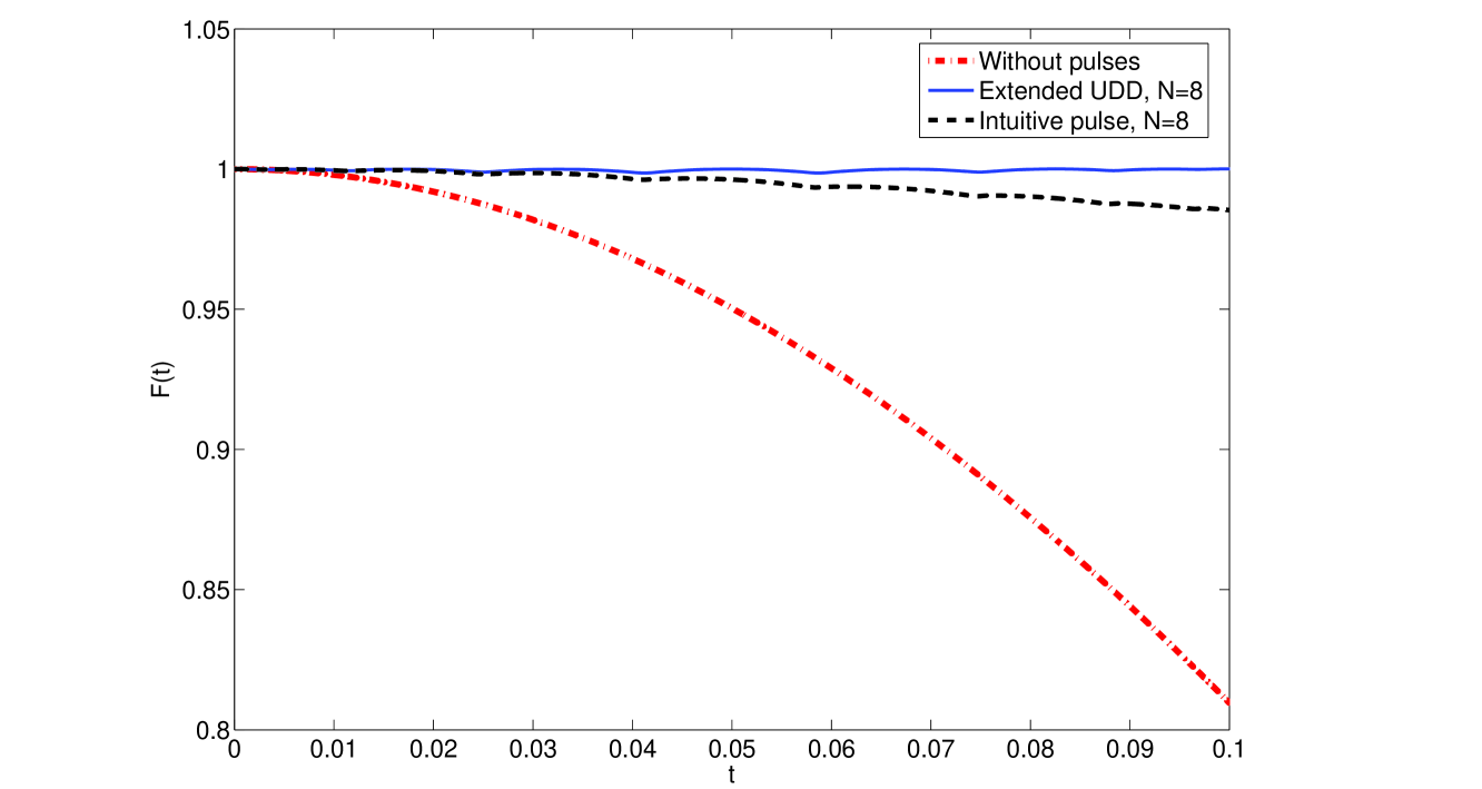
Figure 1: (color online) Expectation value of the coherence measure ${\cal P}_{|\Psi\rangle}$, denoted $F(t)$, as a function of time in dimensionless units, with $|\Psi\rangle$ being the non-entangled state ${|\uparrow\uparrow\rangle}$ of a two-qubit system. The bath responsible for the decoherence is modeled by a three-spin system detailed in the text. The bottom curve is without any control and the decoherence is significant. The middle curve is calculated from a control Hamiltonian intuitively based on two independent qubits. The top solid curve represents significant decoherence suppression due to our two-qubit UDD control Hamiltonian described by Eq. (19).

To further confirm the UDD control sequences we explicitly constructed above, we have performed some simple numerical experiments. We first consider a model of a two-spin system coupled to a bath of three spins. The total Hamiltonian in dimensionless units is hence given by

$$H = \sum_{m=3}^{5}\sum_{j=\{x,y,z\}}b_{j,m}\sigma_{j}^{m}$$ (56)

$$+\sum_{n=1}^{5}\sum_{k=\{x,y,z\}}\sum_{m>n}^{5}\sum_{j=\{x,y,z\}}c_{jk}\sigma_{j}^{m}\sigma_{k}^{n}$$

$$+\ H_{c},$$

where the first two spins constitute the two-qubit system in the absence of any external field, $H_{c}$ represents the UDD control Hamiltonian, and the coefficients $b_{j,m}$ and $c_{jk}$ take randomly chosen values in $[0,1]$ in dimensionless units. In addition, to be more realistic, we replace the instantaneous $\delta(t-T_{j})$ function in our control Hamiltonians by a Gaussian pulse, i.e., $(1/c\sqrt{\pi})e^{-[(t-T_{j})^{2}/c^{2}]}$, with $c=T/100$ unless specified otherwise. Further, we set $T=0.1$, because this scale is comparable to the decoherence time scale.

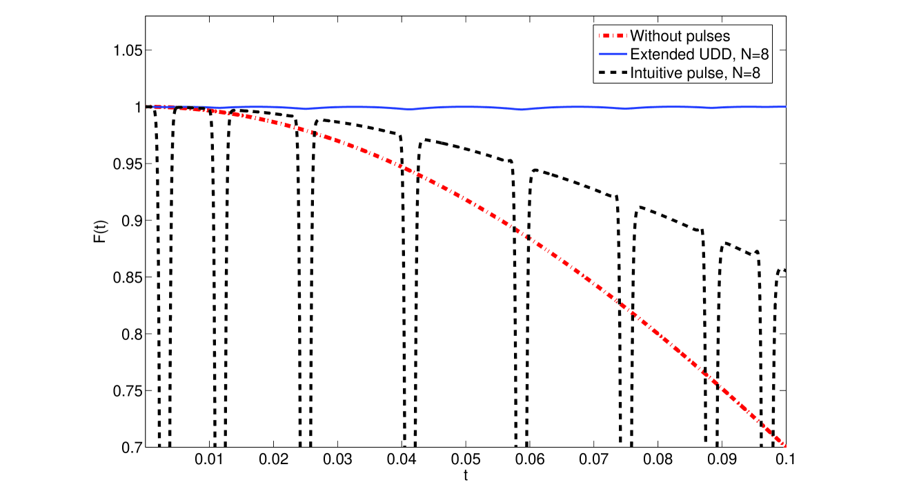
Figure 2: (color online) Same as in Fig. 1, but for ${\cal P}_{|\Psi\rangle}$ associated with a Bell state defined in Eq. (26). The smooth dashed curve represents significant decoherence without control. The drastically oscillating dashed curve is calculated from an intuitive single-qubit-based control Hamiltonian, showing strong population transfer from the initial state to other two-qubit states. The top solid curve represents signficant decoherence suppression due to our two-qubit UDD control sequence in Eq. (32).

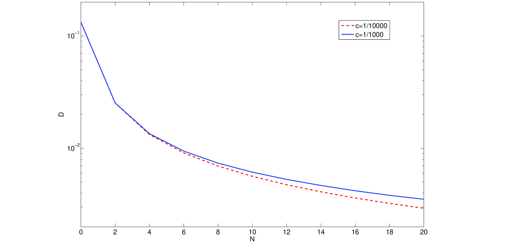
Figure 3: (color online) The time-averaged distance $D$ between the actual density matrix from that of a completely locked Bell state, for $c=T/100$ and $c=T/1000$, versus the number of UDD pulses. The initial state is the same as in Fig. 2.

Figure 1 depicts the time dependence of the expectation value of the coherence measure ${\cal P}_{|\Psi\rangle}$, denoted $F(t)$, with $|\Psi\rangle$ being the non-entangled state ${|\uparrow\uparrow\rangle}$ of the two-qubit system. The initial state of the system is also taken as the non-entangled state ${|\uparrow\uparrow\rangle}$. As is evident from the uncontrolled case (bottom curve) , the decoherence time scale without any decoherence suppression is of the order 0.1 in dimensionless units. Turning on the two-qubit UDD control sequence described by Eq. (19) for $N=8$, the decoherence (top solid curve) is seen to be greatly suppressed. We have also examined the decoherence suppression using a UDD sequence based on the single-qubit-based intuitive control Hamiltonian $H_{c,\text{single}}$ described by Eq. (25). As shown in Fig. 1, $H_{c,\text{single}}$ can only produce unsatisfactory decoherence suppression.

Similar results are obtained in Fig. 2, where we aim to preserve the coherence measure ${\cal P}_{|\Psi\rangle}$ associated with the Bell state defined in Eq. (26). Apparently, with the assistance of our two-qubit UDD control sequence, the system is seen to be locked on the Bell state with a fidelity close to unity at all times. Figure 2 also presents the parallel result if the control Hamiltonian is given by $H_{c,\text{single}}$ shown in Eq. (25). The drastic oscillation of $F(t)$ in this case indicates that strong population oscillation occurs, thereby demonstrating again the difference between single-qubit decoherence suppression and two-qubit decoherence suppression.

Using the same initial state as in Fig. 2, Fig. 3 depicts $\overline{D}\equiv\frac{1}{2T}\int_{0}^{T}||\rho(t)-\rho_{i}||dt$, i.e., the time-averaged distance between the actual time-evolving density matrix from that of a completely locked Bell state, for $c=T/100$ and $c=T/1000$, with different number of UDD pulses. It is seen that, at least for the number of UDD pulses considered here, $c=T/100=1/1000$ (about one hundredth of the decoherence time scale) already suffices to preserve a Bell state. That is, there seems to be no need to use much shorter pulses such as $c=T/1000=1/10000$, because the case of $c=T/1000$ (dashed line) in Fig. 3 shows little improvement as compared with the case of $c=T/100$ (solid line). This should be of practical interest for experimental studies of two-qubit decoherence suppression.

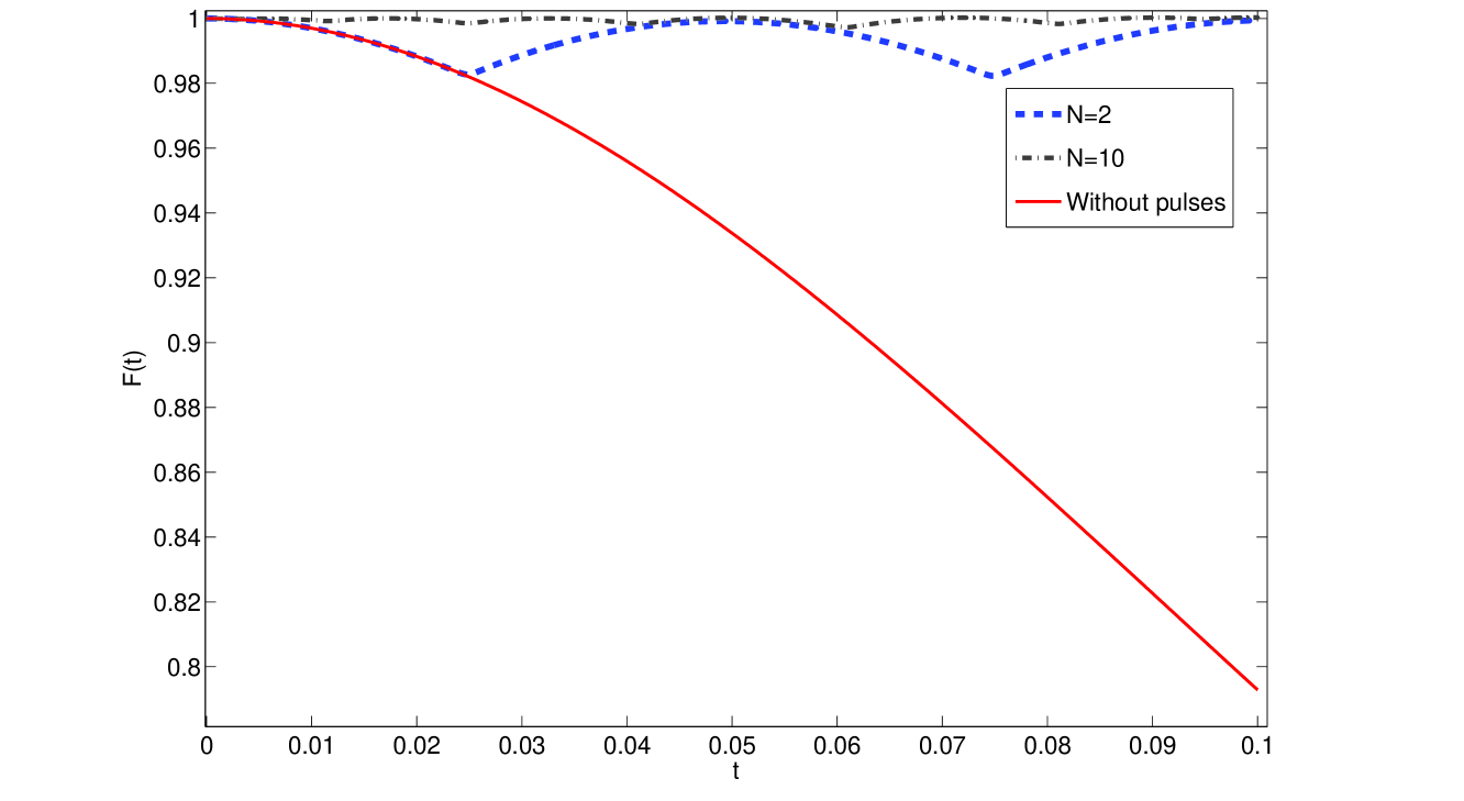
Figure 4: (color online) Expectation value of the coherence measure ${\cal P}_{|\Psi\rangle}$, denoted $F(t)$, as a function of time in dimensionless units, with $|\Psi\rangle$ being one basis state of a three-level system. The central system is coupled with a bath modeled by other four three-level subsystems. The bottom curve represents significant decoherence without decoherence control. The top two curves represent decoherence suppression based on the control operator constructed in Eq. (53), for $N=2$ and $N=10$.

Finally, we show in Fig. 4 the decoherence suppression of a three-level quantum system, with the control operator given by Eq. (53). Here the bath is modeled by other four three-level subsystems, and the total Hamiltonian is chosen as

$$H = \sum_{m=2}^{5}\sum_{\alpha=\{x,y,z\}}b_{j,m}j_{\alpha,m}$$ (57)

$$+\sum_{n=1}^{5}\sum_{\alpha=\{x,y,z\}}\sum_{m>n}^{5}\sum_{\beta=\{x,y,z\}}c_{\alpha\beta}j_{\alpha,m}j_{\beta,n}$$

$$+\ H_{c},$$

where $j_{\alpha,m}$ represents the $j_{x}$, $j_{y}$, or $j_{z}$ operator associated with the $m$th three-level subsystem, with the first being the central system and the other four being the bath. The coupling coefficients are again randomly chosen from $[0,1]$ with dimensionless units. The results are analogous to those seen in Fig. 1 and Fig. 2, confirming the general applicability of our UDD control sequence in multi-level quantum systems. Note also that even for the $N=2$ case (middle curve in Fig. 4), decoherence suppression already shows up clearly. The results here may motivate experimental UDD studies using systems analogous to the kicked-top system realized in Ref. Jessen .

IV Discussion and Conclusion

So far we have assumed that the system-bath coupling, the bath self-Hamiltonian, and the system Hamiltonian in the absence of the control sequence are all time-independent. This assumption can be easily lifted. Indeed, as shown in a recent study by Pasini and Uhrig for single-qubit systems Pasini , the UDD result holds even after introducing a smooth time dependence to these terms. The proof in Ref. Pasini is also based on Yang and Liu’s work univUDD . A similar proof can be done for our extension here. Take the two-qubit case with the control operator $Y_{1}$ as an example. If $H_{0}$ and $H^{\prime}$ are time-dependent, then the unitary evolution operator in Eq. (20) is changed to

$$U(T) = (-iY_{1})^{N}\mathfrak{J}\left[e^{-i\int_{T_{N}}^{T}[H_{0}+(-1)^{N}H^{\prime}]dt}\right]$$

$$\ \times\ \mathfrak{J}\left[e^{-i\int_{T_{N-1}}^{T_{N}}[H_{0}+(-1)^{N-1}H^{\prime}]dt}\right]$$

$$\ \cdots$$

$$\ \times\ \mathfrak{J}\left[e^{-i\int_{T_{2}}^{T_{3}}[H_{0}+H^{\prime}]dt}\right]$$

$$\ \times\ \mathfrak{J}\left[e^{-i\int_{T1}^{T2}[H_{0}-H^{\prime}]dt}\right]$$

$$\ \times\ \mathfrak{J}\left[e^{-i\int_{0}^{T_{1}}[H_{0}+H^{\prime}]dt}\right]$$

$$= (-iY_{1})^{N}\mathfrak{J}\left[e^{-i\int_{0}^{T}H_{0}dt}\right]\mathfrak{J}\left[e^{-i\int_{0}^{T}F_{N}(t)H_{I}^{\prime}(t)\mathrm{d}t}\right],$$

with

$$H_{I}^{\prime}(t)=\mathfrak{J}\left[e^{i\int_{0}^{T}H_{0}dt}\right]H^{\prime}\mathfrak{J}\left[e^{-i\int_{0}^{T}H_{0}dt}\right].$$ (59)

Because the term $\mathfrak{J}\left[e^{-i\int_{0}^{T}H_{0}dt}\right]$ in Eq. (LABEL:uorder) does not affect the expectation value of our coherence measure, the final expression for the coherence measure is essentially the same as before and is hence again given by its initial value multiplied by $1+O(T^{N+1})$.

Our construction of the UDD control sequence is based on a pre-determined coherence measure ${\cal P}_{|\Psi\rangle}$ that characterizes a certain type of quantum coherence. This implies that our two-qubit UDD relies on which type of decoherence we wish to suppress. Indeed, this is a feature shared by Uhrig’s work UDDprl and the Yang-Liu universality proof univUDD for single-qubit systems (i.e., suppressing either transverse decoherence or longitudinal population relaxation). Can we also efficiently suppress decoherence of different types at the same time, or can we simultaneously preserve the quantum coherence associated with entangled states as well as non-entangled states? This is a significant issue because the ultimate goal of decoherence suppression is to suppress the decoherence of a completely unknown state and hence to preserve the quantum coherence of any type at the same time. Fortunately, for single-qubit cases: (i) there are already good insights into the difference between decoherence suppression for a known state and decoherence suppression for an unknown state lorenza3 ; lorenza4 (with un-optimized DD schemes); and (ii) a very recent study QDD showed that suppressing the longitudinal decoherence and the transverse decoherence of a single qubit at the same time in a “near-optimal” fashion is possible, by arranging different control Hamiltonians in a nested loop structure. Inspired by these studies, we are now working on an extended scheme to achieve efficient decoherence suppression in two-qubit systems, such that two or even more types of coherence properties can be preserved. Thanks to our explicit construction of the UDD control sequence for non-entangled and entangled states, some interesting progress towards this more ambitious goal is being made. For example, we anticipate that it is possible to preserve two types of quantum coherence of a two-qubit state at the same time, if we have some partial knowledge of the initial state.

It is well known that decoherence effects on two-qubit entanglement can be much different from that on single-qubit states. One current important topic is the so-called “entanglement sudden death” science , i.e., how two-qubit entanglement can completely disappear within a finite duration. Since the efficient preservation of two-qubit entangled states by UDD is already demonstrated here, it becomes certain that the dynamics of entanglement death can be strongly affected by applying just very few control pulses. In this sense, our results on two-qubit systems are not only of great experimental interest to quantum entanglement storage, but also of fundamental interest to understanding some aspects of entanglement dynamics in an environment.

To conclude, based on a generalized polarization operator as a coherence measure, we have shown that UDD also applies to two-qubit systems and even to arbitrary multi-level quantum systems. The associated control fidelity is still given by $1+O(T^{N+1})$ if $N$ instantaneous control pulses are applied. This extension is completely general because no assumption on the environment is made. We have also explicitly constructed the control Hamiltonian for a few examples, including a two-qubit system and a three-level system. Our results are expected to advance both theoretical and experimental studies of decoherence control.

V Acknowledgments

This work was initiated by an “SPS” project in the Faculty of Science, National University of Singapore. We thank Chee Kong Lee and Tzyh Haur Yang for discussions. J.G. is supported by the NUS start-up fund (Grant No. R-144-050-193-101/133) and the NUS “YIA” (Grant No. R-144-000-195-101), both from the National University of Singapore.

References

• (1) L. Viola and S. Lloyd, Phys. Rev. A 58, 2733 (1998).
• (2) L. Viola, E. Knill, and S. Lloyd, Phys. Rev. Lett. 82, 2417 (1999).
• (3) J. J. L. Morton et al., Nature Physics 2, 40 (2006); J. J. L. Morton et al., Nature 455, 1085 (2008).
• (4) G. S. Uhrig, New Journal of Physics 10, 083024 (2008).
• (5) K. Khodjasteh and D.A. Lidar, Phys. Rev. Lett. 95, 180501 (2005).
• (6) K. Khodjasteh and D. A. Lidar, Phys. Rev. A 75, 062310 (2007).
• (7) G. S. Uhrig, Phys. Rev. Lett. 98, 100504 (2007).
• (8) B. Lee, W. M. Witzel, S. Das Sarma, Phys. Rev. Lett. 100, 160505 (2008).
• (9) M. J. Biercuk, H. Uys, A. P. VanDevender, N. Shiga, W. M. Itano, and J. J. Bolinger, Nature 458, 996 (2009).
• (10) M. J. Biercuk, H. Uys, A. P. VanDevender, N. Shiga, W. M. Itano, and J. J. Bolinger, Phys. Rev. A79, 062324 (2009).
• (11) J. F. Du, X. Rong, N. Zhao, Y. Wang, J. H. Yang, and R. B. Liu, Nature 461, 1265 (2009).
• (12) W. Yang and R. B. Liu, Phys. Rev. Lett. 101, 180403 (2008).
• (13) S. Chaudhury, A. Smith, B. E. Andersdon, S. Ghose, and P. S. Jessen, Nature 461, 768 (2009).
• (14) F. Haake, Quantum Signatures of Chaos 2nd Ed. (Springer-Verlag, Berlin, 1999).
• (15) See, for example, J. Wang and J. B. Gong, Phys. Rev. Lett. 102, 244102 (2009) for an extensive list of the kicked-top model literature and its relevance to several areas.
• (16) S. Pasini and G. S. Uhrig, arXiv:0910.0417 (2009).
• (17) W. X. Zhang, N. P. Konstantinidis, V. V. Dobrovitski, B. N. Harmon, L. F. Santos, and L. Viola, Phys. Rev. B77, 125336 (2008).
• (18) W. X. Zhang, V. V. Dobrovitski, L. F. Santos, L. Viola, and B.N. Harmon, Phys. Rev. B75, 201302 (R) (2007).
• (19) J. R. West, B. H. Fong, and D. A. Lidar, arXiv:0908.4490v2 (2009).
• (20) T. Yu and J. H. Eberly, Science 323, 598 (2009).