Nonequilibrium dynamics of a stochastic model of anomalous heat transport: numerical analysis

Abstract

We study heat transport in a chain of harmonic oscillators with random elastic collisions between nearest-neighbours. The equations of motion of the covariance matrix are numerically solved for free and fixed boundary conditions. In the thermodynamic limit, the shape of the temperature profile and the value of the stationary heat flux depend on the choice of boundary conditions. For free boundary conditions, they also depend on the coupling strength with the heat baths. Moreover, we find a strong violation of local equilibrium at the chain edges that determine two boundary layers of size $\sqrt{N}$ (where $N$ is the chain length), that are characterized by a different scaling behaviour from the bulk. Finally, we investigate the relaxation towards the stationary state, finding two long time scales: the first corresponds to the relaxation of the hydrodynamic modes; the second is a manifestation of the finiteness of the system.

1 Introduction

The problem of heat transport in chains of oscillators is one of the most relevant testing grounds to understand the behaviour of statistical systems steadily kept out of equilibrium. In the last decade, numerical simulations and analytic arguments have contributed to clarify the behaviour of such systems in the thermodynamic limit (see review papers [BLR00, LLP03, DHAR09] and references therein). However, there is still a number of open questions such as the role of Boundary Conditions (BC in the following) and the convergence towards the stationary state. In spite of the continuous increase of computer performances, direct numerical simulations are still not so effective as to provide reliable data on sufficiently large systems. In this respect, stochastic models like the one introduced in [BBO06] prove very helpful. In this paper we consider a version of such models already analyzed in [DLLP08, LMMP09]. The model consists in a chain of $N$ coupled harmonic oscillators in interaction (at the boundaries) with two stochastic heat baths at different temperatures. In addition, the oscillators are subject to stochastic collisions that exchange the momenta of randomly chosen pairs of neighbouring oscillators, so that both energy and momentum are conserved. In a sense, collisions simulate the presence of nonlinear terms, as they contribute to ensuring ergodicity of an otherwise integrable model. In fact, it has been observed that this model closely reproduces the behaviour of standard nonlinear systems such as an FPU-$\beta$ chain, starting from an anomalous (diverging) heat conductivity [DLLP08]. On the other hand, being the collision rule a perfectly linear process, the evolution equations for ensemble averages of the relevant observables can be written in an exact form and thereby solved numerically, without having to deal with the statistical fluctuations that affect finite samples. As a result, we have found that the invariant measure can be effectively approximated by the product of Gaussian distributions aligned along the eigendirections of the covariance matrix [DLLP08]. Moreover, in [LMMP09], we investigated the continuum limit (which corresponds to the large-$N$ limit) of the covariance matrix, deriving suitable partial differential equations for the stationary state, in the case of fixed BC. As a result, we have obtained explicit formulae for the temperature profile and the energy current. Remarkably, this is the first example of an analytic expression for the temperature profile in a system characterized by anomalous heat transport.

In [partI] we go beyond, by extending the continuum limit to include the time dependence of the covariance matrix. The reader is thus referred to [partI] for a more detailed introduction and the corresponding bibliography. The aim of this paper is to complement the analysis contained in [partI] with accurate numerical studies of finite samples with the goal of clarifying those issues that are too difficult to be worked out analytically. We start by numerically computing the stationary covariance for both free and fixed BC. This helps to shed some light on the nontrivial role played by BC, whenever heat transport exhibits an anomalous behaviour. In the presence of normal transport, one expects that BC affect only a finite boundary layer so that, in the thermodynamic limit the leading term of the heat flux is independent of BC. On the other hand, it is known that in disordered chains of linear oscillators, the same system may even behave as a thermal superconductor or as an insulator, by simply switching from free to fixed BC [PRep]. In generic nonlinear chains, numerical simulations suggest that the heat flux scales in the same way, independently of BC. However, the careful simulations performed in [Comm] revealed that in the FPU-$\beta$ model, the ratio between the heat fluxes measured for free and fixed BC does not converge to 1 for $N\to\infty$. Here we show that the same behaviour occurs in our stochastic model. Actually the dependence on BC is even more subtle than one could have imagined: while in the case of fixed BC, the heat flux and the temperature profile are asymptotically independent of the coupling strength with the thermal baths, the same is not true for free BC.

A second objective of this paper is the analysis of the convergence towards the steady state. This question, which has been hardly discussed in the literature, can be straightforwardly addressed for our model, as it amounts to computing the eigenvalues of the evolution operator for the covariances. Moreover, we also compare the convergence of the average heat flux for different system sizes to show how careful direct simulations must be, if they have to be trusted. We find that finite–size effects associated with the relaxation rates of slow, i.e. long-wavelength, modes significantly modify the asymptotic scaling of the relaxation process. In practice, we find numerical evidence that the theoretical hydrodynamic scaling holds only over a finite range of time scales, although its duration diverges with $N$.

The paper is organized as follows. In Section 2, we briefly recall the definition of the covariance matrix, and the coupled equations governing its evolution towards the stationary value. Some properties of the steady state are discussed in Section 3. The problem of the approach to the steady state is addressed in Section LABEL:sec:relax. Finally, in Section LABEL:sec:concl we summarize our main results.

2 Equations for the covariance matrix

In this section, we introduce the minimal notations and definitions needed to follow the main discussion presented in the following sections. The reader interested in a more detailed presentation is referred to [partI]. We consider a chain of $N$ unit-mass particles interacting via nearest-neighbour harmonic coupling of frequency $\omega$. The equations of motion are given by

$$\halign to=0.0pt{\MH@restoretag\MHs@tr@m\hfil$\MH@lign\displaystyle{\MHsh@rp}$&\MHdecrt@t$\MH@lign\displaystyle{{}\MHsh@rp}$&\hfil\MHdecrt@t$\MH@lign\displaystyle{\MHsh@rp}$&\MHdecrt@t$\MH@lign\displaystyle{{}\MHsh@rp}$\hfil&\my@MHput{\MHsh@rp}\cr&\dot{q}_{n}&=&p_{n}{}&\cr&\dot{p}_{n}&=&\omega^{2}(\tilde{\delta}_{n,N}q_{n+1}-2q_{n}+\tilde{\delta}_{n,1}q_{n-1})+\delta_{n,1}(\xi^{+}-\lambda\dot{q}_{1})+\delta_{n,N}(\xi^{-}-\lambda\dot{q}_{N})\ ,{}&\cr}$$

where $p_{n}$, $q_{n}$ are the momentum and displacement from equilibrium position of the $n$-th particle, $\delta_{i,j}$ is the Kronecker delta and $\tilde{\delta}_{i,j}\equiv 1-\delta_{i,j}$, and $\xi^{\pm}$ are independent Wiener processes with zero mean and variance $2\lambda k_{B}T_{\pm}$, where $k_{B}$ is the Boltzmann constant and $\lambda$ is the coupling constant. In the following free and fixed boundary conditions will be considered. These can be expressed in terms of the position variable $q$ as: $q_{0}=q_{1}$, $q_{N}=q_{N+1}$ for free BC and $q_{0}=q_{N+1}=0$ for fixed BC.

We consider the covariance matrix written as

$$\mathbf{c}=\left(\begin{array}[]{cc}\mathbf{y}&\mathbf{z}\\ \mathbf{z}^{\dagger}&\mathbf{v}\end{array}\right)\ .$$ (1)

where the matrices $\mathbf{y}$, $\mathbf{z}$ and $\mathbf{v}$, of respective dimension $(N-1)\!\times\!(N-1)$, $(N-1)\!\times\!N$ and $N\!\times\!N$ are defined as

$$\mathbf{y}_{i,j}=\langle\Delta q_{i}\Delta q_{j}\rangle\ ,\\ \mathbf{z}_{i,j}=\langle\Delta q_{i}p_{j}\rangle\ ,\\ \mathbf{v}_{i,j}=\langle p_{i}p_{j}\rangle\ ,\\$$ (2)

where $\langle\cdot\rangle$ denotes the average over phase space probability distribution function $P$ and $\Delta q_{i}=q_{i}-q_{i-1}$ stand for the particle relative displacements. The variables $(\Delta q_{i},p_{i})$ are the convenient choice to deal with: one the one hand, absolute positions are not well defined for free BC and on the other hand, the potential energy is expressed in terms of relative differences. The only subtlety is that the domain of definition of $\Delta q_{i}$ differs from that of $p_{i}$. Thereby, the bulk of the system is defined as $\{\Delta q_{i}\ |\ i\in[2,N]\}$ and $\{p_{i}\ |\ i\in[2,N-1]\}$. The evolution equations for $\mathbf{c}$ in the bulk are

$$\halign to=0.0pt{\MH@restoretag\MHs@tr@m\hfil$\MH@lign\displaystyle{\MHsh@rp}$&\MHdecrt@t$\MH@lign\displaystyle{{}\MHsh@rp}$&\hfil\MHdecrt@t$\MH@lign\displaystyle{\MHsh@rp}$&\MHdecrt@t$\MH@lign\displaystyle{{}\MHsh@rp}$\hfil&\my@MHput{\MHsh@rp}\cr&\dot{\mathbf{y}}_{i,j}&\ =&\mathbf{z}_{j,i}-\mathbf{z}_{j,i-1}+\mathbf{z}_{i,j}-\mathbf{z}_{i,j-1}\ ,{}&\cr&\dot{\mathbf{z}}_{i,j}&\ =&\mathbf{v}_{i,j}-\mathbf{v}_{i-1,j}+\omega^{2}\left(\mathbf{y}_{i,j+1}-\mathbf{y}_{i,j}\right)+\gamma\left(\mathbf{z}_{i,j+1}+\mathbf{z}_{i,j-1}-2\mathbf{z}_{i,j}\right)\ ,{}&\cr&\dot{\mathbf{v}}_{i,j}&\ =&\omega^{2}\left(\mathbf{z}_{j+1,i}-\mathbf{z}_{j,i}+\mathbf{z}_{i+1,j}-\mathbf{z}_{i,j}\right)+\gamma\mathbf{W}_{i,j}\ .{}&\cr}$$

These equations follow from the deterministic equations of motion (LABEL:eq:eqs-motion) plus the contribution of the stochastic noise ($\gamma$ denotes the collision rate), that is described by the collision matrix $\mathbf{W}$,

$$\mathbf{W}_{ij}\equiv\left\{\begin{array}[]{ll}\mathbf{v}_{i-1,j-1}+\mathbf{v}_{i+1,j+1}-2\mathbf{v}_{i,j}&i=j\\ \mathbf{v}_{i-1,j}+\mathbf{v}_{i,j+1}-2\mathbf{v}_{i,j}&i-j=-1\\ \mathbf{v}_{i+1,j}+\mathbf{v}_{i,j-1}-2\mathbf{v}_{i,j}&i-j=1\\ \mathbf{v}_{i+1,j}+\mathbf{v}_{i-1,j}+\mathbf{v}_{i,j-1}+\mathbf{v}_{i,j+1}-4\mathbf{v}_{i,j}&|i-j|>1\end{array}\right.\ .$$ (3)

On the boundaries, several changes appear in the velocity fields. The interested reader can find a full description in Section 2.2 of [partI]. Here we limit ourselves to show the contribution arising from the coupling with the heat bath, namely

$$\dot{\mathbf{z}}^{b}_{i,j} = \delta_{j,1}\mathbf{z}_{i,1}+\delta_{j,N}\mathbf{z}_{i,N}\ ,$$

$$\dot{\mathbf{v}}^{b}_{i,j} = \delta_{j,1}\mathbf{v}_{i,1}+\delta_{j,N}\mathbf{v}_{i,N}+\delta_{i,1}\mathbf{v}_{1,j}+\delta_{i,N}\mathbf{v}_{N,j}-2\left(T^{+}\delta_{i,1}\delta_{j,1}+T^{-}\delta_{i,N}\delta_{j,N}\right)\ .$$

3 Stationary covariance

In this section we investigate some properties of the nonequilibrium steady state, for both fixed and free BC. The stationary state is obtained by considering the time-independent solution of equations (LABEL:eq:Cdot). It can be efficiently determined by exploiting the sparsity of the corresponding linear problem, as well as the symmetries of the unknowns (this approach has been followed in [DLLP08] for fixed BC). Alternatively, one can just let evolve equations (LABEL:eq:Cdot) starting from any meaningful initial conditions, as the dynamics will necessarily converge towards the only stable stationary state (here we have adopted this latter approach also because we wish to study the convergence – see in the following). All numerical results presented in this paper have been obtained for $\omega=1$, $T_{+}=1.5$, $T_{-}=0.5$. This is by no means a limitation, as all these parameters can be easily scaled out due to the linear structure of the model. Accordingly, they will not be mentioned again, unless specifically needed for a comparison with theoretical predictions.

3.1 The heat flux

The first observable we have looked at is the energy flux at position $i$ which, in terms of the matrices $\mathbf{v}$, $\mathbf{z}$ is written as [PRep]

$$J_{i}=-\omega^{2}\mathbf{z}_{i+1,i+1}+\frac{\gamma}{2}(\mathbf{v}_{i,i}-\mathbf{v}_{i+1,i+1}).$$ (4)

We have adopted the convention that a positive flux corresponds to a propagation towards increasing values of the spatial index $i$. The first term stems from the deterministic forces and provides for the leading (anomalous) contribution, while the second one accounts for energy exchanges due to collisions of nearby particles. In the stationary state, $J_{i}$ is independent of $i$, i.e. $J_{i}\equiv J$ .

In figure 1 we show $J\sqrt{N}$ as a function of the inverse of the system size $N$. The results refer to free BC (as we do not have analytic estimates to compare with), $\lambda=1$ and different values of the collision rate $\gamma$ (see the various symbols as described in the figure caption). In all cases there is a convincing evidence that $J\sim N^{-1/2}$, similar to what predicted analytically in [LMMP09] for the case of fixed BC. As a consequence, the effective conductivity, $\kappa\equiv JN/(T_{+}-T_{-})$ diverges as $\sqrt{N}$. However, from figure 1 it is also evident the presence of sub-leading singular corrections which hinder the extrapolation of the asymptotic value. In analogy to [LMMP09], we introduce the Ansatz,

$$J\;=\;\frac{{\mathcal{J}}}{\sqrt{N}}+\frac{B}{N^{\beta}}$$ (5)

By using this formula to fit the data, we obtain the curves reported in figure 1 which reproduce quite well the raw data. Notice that the convergence is from below for smaller $\gamma$ values, while from above for larger collision rates. All the estimated $\beta$ values range in the interval $[0.88,0.95]$, suggesting that this parameter may be “universal”.

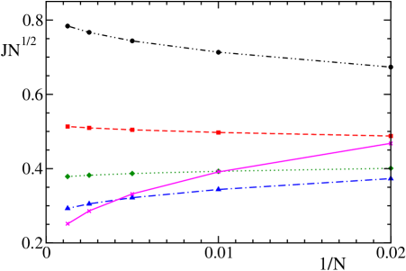
Figure 1: Free BC ($\lambda=1$): the scaled stationary flux $J\sqrt{N}$ versus $1/N$ for $\gamma$=0.2 (circles), 0.5 (squares), 1 (diamonds), 2 (triangles), 5 (crosses). The lines are obtained by fitting the data with equation (5).

The extrapolated ${\mathcal{J}}$ values are plotted in figure  2, where we can see that ${\mathcal{J}}\sim\gamma^{-1/2}$, as found for fixed BC [LMMP09] . For $\gamma=5$, the extrapolated value of ${\mathcal{J}}$ suffers a substantial uncertainty due to large finite-size corrections (that become even more sizeable for yet larger $\gamma$ values).

Figure 2: Asymptotic value of ${\mathcal{J}}$ as a function of the collision rate $\gamma$ for free BC and the same parameter values as in figure 1. Data are plotted in log-log scales. The error bar for $\gamma=5$ has been estimated from a rough comparison among different extrapolation schemes. The dashed line is a power law fit of the first four data: its slope is -0.51. The solid line corresponds to the analytic solution for fixed BC (equation (20) of [LMMP09]).

So far, we have not found any relevant difference between fixed and free BC. The heat flux scales in the same way in both cases and exhibits the same dependence on the collision rate. If the effect of the BC were restricted to a layer of finite width around the boundary, in the thermodynamic limit, the thermal resistance of a given chain would be independent of the type of thermal contact. In other words, we should expect ${\mathcal{J}}$ to be independent of the BC. However, this is not the case, as it can be inferred from figure  2, where we have also plotted the analytic curve for the fixed BC case (equation (20) in [LMMP09]). For free BC, the heat flux is approximately twice as that obtained for fixed BC. It is worth mentioning that the same effect was found in the simulations of FPU-$\beta$ chains [Comm], although with a slightly different value of the ratio (around 1.7 in that case). Since the flux is constant along the chain, this means that even deeply in the bulk, the system perceives the effect of the boundaries. In particular, from the knowledge of the local temperature profile and from the heat flux, one can in principle infer the type of BC. These results suggest that this is another way anomalous conduction manifests itself.

The whole scenario is even more subtle than suggested by figure 2. In fact, for free BC, the leading term of the heat flux depends not only on $\gamma$ but also on the coupling strength $\lambda$ with the heat bath, while this is not so for fixed BC. We illustrate this in figure 3, where we plot the ratio

$$j_{r}=j(\lambda=1,N)/j(\lambda=1/4,N)$$ (6)

where $j(\lambda,N)$ is the heat flux in a chain of length $N$ and for a given value of $\lambda$. It is not surprising to see that the coupling with the heat baths modifies the flux in chains of finite length. However, we see that for fixed BC, the effect of the coupling vanishes as $j_{r}$ converges to 1 (see the lower curve in figure  3). On the contrary, for free BC, $j_{r}$ remains significantly different from 1. This suggests that fixed BC may lead to a kind of universal behaviour, namely the heat flux and also the temperature profile are independent of the details of the coupling with the heat baths. This is not the case for free BC. It would be interesting to check whether the same holds true in generic nonlinear chains.

Figure 3: Ratio of the energy fluxes as defined in equation (6), for free (diamonds) and fixed (circles) BC as a function of $1/\sqrt{N}$, and for $\gamma=1$. The error on $j_{r}$ for free BC and $N=1600$ is due to a not yet relaxed dynamics.

3.2 The temperature profile

Another observable of interest is the temperature profile $T_{i}=\langle p^{2}_{i}\rangle$. In figure 4 we show the temperature profile for free BC and three different sizes, as a function of the “normalized” position along the chain $y\equiv 2i/N-1$, that varies in the interval $[-1,1]$. The data collapse is coherent with the scaling assumed in the continuum approach [LMMP09]. The shape of the profile is qualitatively similar to that obtained for fixed BC but, although here there are no (square-root) singularities at the boundaries of the chain (see equation (19) and (79) in [LMMP09]). Furthermore, we notice that the profile itself depends on both $\gamma$ and $\lambda$. Evidence of such a dependence can be appreciated in the the inset of figure 4, where the difference $\delta T(y)$ between the profiles corresponding to $\lambda=1$ and $1/4$ is plotted in for three different system sizes. In fact, we see that $\delta T(y)$ does not vanish in the thermodynamic limit. Moreover, the regions around the boundaries are affected by strong finite-size effects. In fact, one expects that $\delta T(-1)=\delta T(1)=0$, as the temperature necessarily converges, as $N\rightarrow\infty$, to that of the attached heat bath.

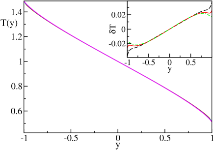
Figure 4: Temperature profile $T(y)$ for $\gamma=1$ and $\lambda=1$ and free BC, for $N$ = $100$, $200$, $400$ and $800$. In the inset: the relative difference between the temperature profiles corresponding to $\lambda=1$ and $\lambda=1/4$, with $\gamma=1$ and for $N=400$, $800$, and $1600$ (dashed, solid, and dotted-dashed lines, respectively).

3.3 Other correlators

In this section we analyse the behaviour of the different correlators (2), along the diagonal ($i=j$) and for generic values of $x=(i-j)/\sqrt{N}$. We first analyse the case of fixed BC.

At equilibrium, off-diagonal elements of the correlators (2) are zero. In the nonequilibrium steady state we have recently shown that the off-diagonal correlators $\mathbf{v}$ are of $\Or(1/\sqrt{N})$ [LMMP09]. This is confirmed in figure 5a, where we plot the lower diagonal of $\mathbf{v}_{i,i+1}$, corresponding to $\mathbf{v}$ measured at a distance $x=1/\sqrt{N}$ from the diagonal, that is denoted by $x=0^{+}$.

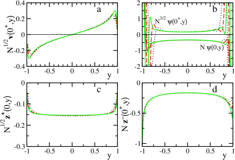
Figure 5: Behaviour of the stationary covariances as a function of the coordinate $y$ for fixed BC and different sizes: (a) First lower diagonal of $\mathbf{v}$ (b) diagonal (lower curves) and first subdiagonal (upper curves) of $\psi$ (c) diagonal of the symmetric component $\mathbf{z}^{+}$ and (d) First subdiagonal of the antisymmetric component $\mathbf{z}^{-}$. In all panels, dotted, dashed and solid lines refer to $N=200$, $400$, and $800$ respectively. The physical parameters are $\gamma=1$, $\lambda=1$.

The potential energy profile $\mathbf{y}$ closely reproduces the kinetic energy profile (see also [DLLP08]). In order to appreciate its contribution, it is necessary to look at higher-order corrections. This can be done by introducing

$$\psi_{i,j}=\mathbf{v}_{i,j}-\omega^{2}\mathbf{y}_{i,j}$$ (7)

which measures the mismatch between kinetic and potential energy. Figure 5b shows that along the diagonal (see the lower set of curves), $\psi$ scales as $1/N$ everywhere except perhaps at the boundaries. From a physical point of view, this implies that everywhere in the bulk, the system is locally at equilibrium (with $1/N$ finite-size deviations from the virial equality). The wild behaviour observed near the boundaries suggests the existence of nontrivial boundary layers. We will discuss this in detail in the next subsection. Analogously to $\mathbf{v}$, $\psi$ exhibits a “discontinuity” when moving away from the diagonal. Indeed, in the upper set of curves of figure 5b we show that $\psi(x=0^{+},y)$ is of order $1/N^{3/2}$. It is worthwhile remarking that this scaling holds only for $\lambda=1$. For$\lambda\neq 1$ we have found that the off-diagonal terms of $\psi$ are of order $1/N$ too. By recalling that we have here selected $\omega=1$ , it is reasonable to conjecture that the faster convergence of $\psi$ observed for $\lambda=1$ is a manifestation of the thermal impedance matching on the boundary, theoretically predicted for $\lambda=\omega$ (see [partI]).

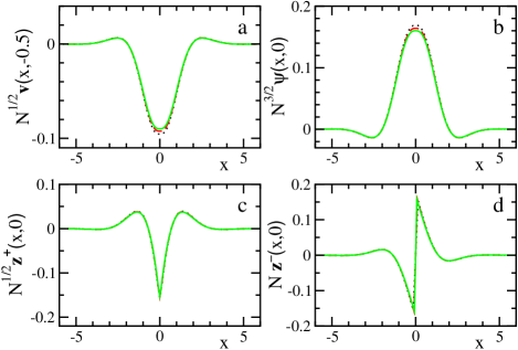
Figure 6: Off-diagonal behaviour of the stationary covariances for fixed BC and the same parameter values and same notations as in the previous figure: (a) $\mathbf{v}$ for $y=-0.5$; (b) $\psi$ for $y=0$; (c) $\mathbf{z}^{+}$ for $y=0$ (d) $\mathbf{z}^{-}$ for $y=0$. The physical parameters are $\gamma=1$ and $\lambda=1$. For the sake of clarity, in panels a and b the diagonal values ($x=0$) are omitted as they are of lower order.

Moreover, as shown in [partI], it is convenient to distinguish between symmetric and anti-symmetric components of the correlators $\mathbf{z}$ with respect to $x$,

$$\mathbf{z}^{\pm}_{i,j}=\frac{\mathbf{z}_{i,j}\pm\mathbf{z}_{j,i}}{2}\ .$$ (8)

In figure 5c, we plot the symmetric component which corresponds to the leading term of the heat flux. In fact, it scales as $1/\sqrt{N}$. The deviations from a perfectly flat shape reveal again the presence of nontrivial boundary layers. Along the diagonal the antisymmetric component $\mathbf{z}^{-}$ is zero by construction, while along the first subdiagonal, $\mathbf{z}^{-}$ scales as $1/N$ (see figure 5d).

In figure 6 we show the behaviour of the correlators as a function of their distance $x$ from the diagonal. We have found that $\mathbf{z}^{-}$ and the derivative of $\mathbf{z}^{+}$ along $x$ are both discontinuous across the diagonal, in agreement with the theoretical analysis in [partI]. All the results are independent of $\lambda$ except for the variable $\psi$ which, for $\lambda\neq 1$, is constant away from the diagonal and of order $1/N$. We would like to remark that this anomaly does not affect the theoretical analysis carried in [LMMP09] and [partI], as (for fixed BC) $\psi$ does not contribute to the leading behaviour of the temperature profile and of the heat flux.

The very good overlap among the curves obtained for different system sizes confirms the scaling behaviour of the off-diagonal already seen in figure 5. Most important, the observed scaling corroborates the validity of the ansatz used in [LMMP09] and [partI]. Summarizing, for fixed BC and far from the boundary we find that:

• Along the diagonal, $\psi$ is $\Or(1/N)$. Off-diagonal, $\psi$ is $\Or(1/N^{3/2})$ for $\lambda=\omega$ and $\Or(1/N)$ otherwise.

• The correlator $\mathbf{v}$ is $\Or(1)$ along the diagonal and $\Or(1/\sqrt{N})$ off-diagonal.

• The symmetric correlator $\mathbf{z}^{+}$ is $\Or(1/\sqrt{N})$ everywhere.

• The antisymmetric correlator $\mathbf{z}^{-}$ is $\Or(1/N)$.

As a final remark, note that $\mathbf{z}^{+}$ is the only variable that is continuous in $x$. This implies that the difference $\mathbf{z}^{+}(0^{+},y)-\mathbf{z}^{+}(0,y)$, that we have denoted by $\delta\mathbf{z}^{+}$ in [partI], must necessary be an order $\varepsilon$ higher than its addenda, since its leading contribution is a derivative with respect to $x$.

We now turn our attention to the free BC. As it can be seen in figure 7, the correlators scale with $N$ in the same manner, irrespectively of the boundary conditions. We only notice the following qualitative differences: First, with free BC, the convergence at the boundaries is more effective than for fixed BC (compare figure 5b with figure 7c). Second, as a function of $x$, some additional oscillations of $\mathbf{z}$ can be seen only for fixed BC (figure 5c and figure 7b). Third, $\mathbf{z}^{+}$ is larger for free BC, in agreement with the fact that in this case, the heat flux is about two times larger than for fixed BC.

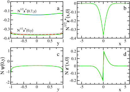
Figure 7: Elements of the stationary covariances for free BC and different sizes: (a) $\mathbf{z}^{+}(x=0,y)$ (lower curves) and at $\mathbf{z}^{+}(x=0.7,y)$ (upper curves); (b) $\mathbf{z}^{+}(x,y=0)$; (c) $\psi(x=0,y)$ (d) $\mathbf{z}^{-}(x,y=0)$. In all panels, dotted, dashed and solid lines refer to $N=200$, $400$, and $800$ respectively.

3.4 Behaviour at the chain edges

The numerical discussion carried out in the previous subsection has revealed the existence of “boundary layers” in the vicinity of the contact points with the heat baths ($y\approx\pm 1$), where strong deviations from the expected scaling behaviour are clearly visible. Since in [partI], we have not attempted a theoretical analysis of the boundary layers, it is at least necessary to clarify their relevance, with reference to the numerical but otherwise exact solutions for the correlators.

The variable that is mostly affected by the presence of such boundary layers is $\psi$ which even changes its scaling behaviour with $N$. This is shown in figure 8 for the case of fixed BC. In order to emphasize the scaling behaviour at the boundary, we subtract from $\psi$ the $1/N$ term (denoted by $\psi_{b}$) in the bulk that we know is constant (see [partI]). For fixed BC and $\lambda=1$, $\psi_{b}=0$, since the leading term is of order $1/N^{3/2}$, while for $\lambda=0.25$, $\psi_{b}=1/N$ (with a few percent of uncertainty on the numerical constant.) The data collapse reveals that $\psi$ passes from values of order $1/\sqrt{N}$ to values of higher order over a number of sites of order $\sqrt{N}$.

Figure 8: Scaling behaviour of $\psi_{i,j}$ close to the leftmost edge of the chain ($y\approx-1$) for fixed BC and $\gamma=1$. Dotted, dashed and solid lines refer to $N=200$, $400$, and $800$ and $\lambda=1$. The three lower (upper) curves correspond to $x=0.7$ ($x=0$). Triangles correspond to $N=1600$, $\lambda=0.25$, and $x=0$.

The existence of a boundary layer manifests itself in the values that different correlators assume at the boundaries (in the vicinity of $y=\pm 1$). At the level of the partial differential equations derived in [partI], the BC (either free or fixed), lead to certain mathematical constraints among the correlators that must be satisfied for $y=\pm 1$. For instance, for free BC, we have found analytically that (see Eqs. (64), (65) and (66) of [partI])

$$\omega^{2}\mathbf{z}^{+}(x,-1)-\lambda\mathbf{v}(x,-1)=0\ ,\ \textrm{and}\quad(\omega^{2}-\lambda^{2})\mathbf{v}(x,-1)-\omega^{2}\psi(x,-1)=0\ .$$

& =

$$Onthecontrary,forfixedBCwehavefoundthatallcorrelatorsturnouttobezeroattheboundaries.Infiguredifwehaveplottedthecombinedvariablesappearinginthel.h.s.of(constraints)for\omega and\gamma unity.Inpanela,weplot𝐳{}^{+}-\lambda 𝐯asafunctionofyfor\lambda =1(dottedanddotted-dashedcurves)and\lambda =1/4(solidanddashedcurves).Inbothcases,thecombinedvariablereacheszeroaty\to -1,thusconfirmingthefindingsin\text{<cite class="ltx\_cite ltx\_citemacro\_cite">[<span class="ltx\_ref ltx\_missing\_citation ltx\_ref\_self">partI</span>]</cite>}.Moreimportantly,for\lambda =1/4,onecaninferthat𝐳{}^{+}-\lambda 𝐯willexhibitadiscontinuityaty=-1inthelimitN\to \mathrm{\infty }.Thisisadirectconsequenceoftheboundarylayerwhichcanbefurtherseeninfiguredifb,whereweplot\psi -(1-\lambda {}^2)𝐯for\lambda =1/4.Furthermore,weseethatthesecondtheoreticalconstraint(constraints)isalsosatisfied.Thismeansthat\psi becomesofthesameorderas𝐯.Fromaphysicalpointofviewthisimpliesthatintheboundarylayer,i.e.atashortdistancefromtheboundaries(oftheorderof\sqrt{N}),localequilibriumdoesnothold.\text{Figure 99Figure 99Theconst}$$