Detecting bispectral acoustic oscillations from inflation using a new flexible estimator
Abstract
We present a new flexible estimator for comparing theoretical templates for the predicted bispectrum of the CMB anisotropy to observations. This estimator, based on binning in harmonic space, generalizes the “optimal” estimator of Komatsu, Spergel, and Wandelt by allowing an adjustable weighting scheme for masking possible foreground and other contaminants and detecting particular noteworthy features in the bispectrum. The utility of this estimator is illustrated by demonstrating how acoustic oscillations in the bispectrum and other details of the bispectral shape could be detected in the future PLANCK data provided that is sufficiently large. The character and statistical weight of the acoustic oscillations and the decay tail are described in detail.
keywords:
cosmic microwave background – early universe – methods: statistical.1 Introduction
At present the primordial blackbody component of the cosmic microwave background (CMB) appears very nearly Gaussian, as one would expect from inflationary models for the very early universe. To a first approximation, because of the weak coupling of the physics involved, inflation predicts a nearly scale-invariant spectrum of primordial density perturbations whose imprint on the CMB is completely characterized by the power spectrum , where is the multipole number and , according to the Gaussian distribution:
| (2) | |||||
where
| (3) |
with denoting temperature and the -mode polarization.
It has however been noted that even in single scalar field inflationary models small nonlinear corrections do arise, at lowest order in the bispectrum (Maldacena, 2003; Acquaviva et al., 2003). In models with several scalar fields even larger and potentially detectable degrees of non-Gaussianity are possible (Bartolo, Matarrese & Riotto, 2002; Rigopoulos, Shellard & Van Tent, 2006, 2007; Naruko & Sasaki, 2009; Byrnes et al., 2008, 2009; Huang, 2009).
Non-Gaussianity manifests itself in odd -point correlation functions or in the connected even -point correlation functions, from which the trivial part expressible as combinations of two-point correlation functions has been subtracted away. The extent of departures from Gaussianity can be characterized by ratios of higher-order correlation functions and the appropriate combination of two-point correlation functions (Bernardeau et al., 2002). The evolution, for the most part linear, of the primordial fluctuations of the inflaton field, involving both gravity and hydrodynamics, leads to CMB anisotropies whose statistical properties mirror those of the primordial fluctuations. Consequently, by studying higher-order correlation functions of the CMB anisotropies, we can detect and characterize any primordial non-Gaussianity.
The lowest order such statistic is the bispectrum, or three-point correlation function in Fourier space. The bispectrum has been shown to be an optimal statistic for measuring non-Gaussianity in the sense that the signal-to-noise squared of the non-Gaussianity estimator based on the three-point correlation function dominates over all higher-order estimators (Babich, 2005). Consequently it would also be significantly easier to constrain. Assuming that the characteristic amplitude of the bispectrum is much larger than that of the trispectrum, or the four-point correlation function in Fourier space, the non-Gaussianity of the density fluctuations from inflation for the single-field case may be approximated by the following “local” ansatz for the gravitational potential (Verde et al., 2000; Komatsu & Spergel, 2001)
| (4) |
where the nonlinearity parameter may be considered small. While the three-point correlator of the linear or Gaussian part is zero (because in the quantum picture it involves the expectation value of a product of three creation and annihilation operators), this is no longer true when the quadratic correction is taken into account. The bispectrum will be proportional to which determines the size of non-Gaussianity. While this form is only approximate for the single-field case, for the observationally more promising multi-field models for which potentially observable values of can be generated, this ansatz is very accurate because the bulk of the non-Gaussianity is imprinted after horizon crossing.
The primordial bispectrum is characterized by an overall amplitude and the shape. Translational and rotational invariance reduce the bispectrum to a function of the lengths only of the three wave vectors. A classification of bispectra shapes has been proposed by Fergusson & Shellard (2009). Local and warm models peak on squeezed triangles, the equilateral models on equilateral triangles, and the folded/flat models on flattened triangles. Models in which perturbations are generated outside the horizon produce a bispectrum that peaks on squeezed triangle configurations, examples of which are multi-field inflation (Lyth, Ungarelli & Wands, 2003; Bartolo, Matarrese & Riotto, 2004; Rigopoulos, Shellard & Van Tent, 2007). [For a review, see Bartolo, Komatsu, Matarrese & Riotto (2004).] The bispectrum of standard single-field inflation can be viewed as a superposition of the local shape and the equilateral shape, both terms, however, being slow-roll suppressed (Maldacena, 2003; Fergusson & Shellard, 2009; Senatore, Smith & Zaldarriaga, 2009). In particular, for the squeezed triangle configurations in single-field inflation the non-Gaussian signal would be proportional to the tilt of the power spectrum and thus imply a strong deviation from scale invariance (Creminelli & Zaldarriaga, 2004b; Cheung et al., 2008). A bispectrum peaking on equilateral triangles is predicted in models with non-standard kinetic terms in the inflaton Lagrangian, which is the case of multi-field inflation models such as DBI inflation (Alishahiha et al., 2004), ghost inflation (Arkani-Hamed et al., 2004) or trapped inflation (Green et al, 2009). Flattened-triangle configurations arise from initial conditions which deviate from the Bunch-Davies vacuum (Holman & Tolley, 2008). The limits for of the local shape from the WMAP5 analysis are at 95% confidence (i.e. ) (Komatsu et al., 2009a).
After horizon crossing, non-linearities in both the gravitational and hydrodynamical evolution of the baryon-photon fluid prior to recombination (Pyne & Carroll, 1996; Bartolo, Matarrese & Riotto, 2004; Creminelli & Zaldarriaga, 2004a; Nitta et al., 2009), as well as higher orders in the gravitational potential during recombination (Bartolo & Riotto, 2008), can generate non-Gaussianity. Other sources of non-primordial non-Gaussianity include secondary anisotropies such as weak lensing via the cross-correlation with the unlensed CMB arising from the integrated Sachs-Wolf effect (Smith & Zaldarriaga, 2006; Hanson et al., 2009; Mangilli & Verde, 2009) or the Sunyaev-Zel’dovich effect (Goldberg & Spergel, 1999), as well as foregrounds such as dust, galactic synchrotron radiation and unresolved point sources. Finally there are also instrumental effects, see e.g. Donzelli et al. (2009). These effects contribute spurious non-Gaussian signals, thus biasing the measurement of the primordial signal. It is therefore important to develop tools to isolate the primordial signal from the contaminants.
The separation of the CMB and foreground components exploits their differing spectral and spatial distribution (Goldberg & Spergel, 2008). It has been shown that foreground sources distributed in an anisotropic manner can mimic a non-Gaussian signal which could be taken for primordial (Carvalho, 2009). It has been suggested that the claimed detection of (Yadav & Wandelt, 2008) might be due to residual foregrounds or instrumental contamination (Pietrobon et al., 2008; Cabella et al., 2009; Smith, Senatore & Zaldarriaga, 2009). Consequently it is important to develop estimators based on the bispectrum also able to mask out non-primordial parasite non-Gaussianities.
In this paper we shall focus primarily on bispectral non-Gaussianity of the “local” type just defined, although most of the discussion generalizes straightforwardly to other templates. See also Fergusson & Shellard (2007, 2009), whose authors are working on another bispectral estimator program, specifically aimed at dealing with theoretical primordial bispectra of general momentum dependence. In fact, their expansion of a general primordial bispectrum in terms of separable eigenfunctions is one way to easily extend our work beyond the “local” type of primordial non-Gaussianity. Unlike much of the literature, where the emphasis is on developing an “optimal” estimator, where all the data are reduced to a single number (Heavens, 1998; Komatsu et al., 2005; Yadav et al., 2008; Creminelli, Senatore & Zaldariaga, 2007), the emphasis in our paper is placed on developing a more flexible approach where the data can be divided in many ways and under which the effects of parasite non-Gaussianities can be masked in a well-defined way. See also Curto, Martínez-González & Barreiro (2009); Lan & Marinucci (2008); Rudjord et al. (2009); Hikage (2008); Munshi & Heavens (2009); Munshi et al. (2009); Santos et al. (2003); Smith, Senatore & Zaldarriaga (2009) for other estimators, many not based on the bispectrum but on wavelets, needlets, or Minkowski functionals.
The paper is organized as follows. In section 2 we establish some notation and discuss some general properties of estimators. A simplified and intuitive discussion of the nature and distribution of statistical weight of the ”local” bispectral signal is given and it is shown how to modify templates in order to best mask parasite contaminants. Section 3 presents a quantitative discussion of the shape of the ”local” signal and in particular the acoustic oscillations are examined quantitatively. In section 4 the signal-to-noise for acoustic oscillations in the vertex region (where ) is examined. Section 5 gives the computational details of a binned bispectral estimator that can be used for a general template and presents tests validating this estimator. Finally in section 6 we present some concluding remarks.
2 Basic Formalism
2.1 Reduced bispectrum
The temperature fluctuations in the CMB can be decomposed into spherical harmonics according to
| (5) |
with the harmonic coefficients given by
| (6) |
The bispectrum on the celestial sphere consists of cubic combinations of the spherical harmonic coefficients of the form
| (7) |
whose expectation values may be calculated for a given theory. However under the assumption of statistical isotropy, these expectation values are not independent and can be reduced to quantities depending only on and In the sequel, we shall not always explicitly indicate expectation values, because in many cases the equations can be interpreted either with expectation values or as relating statistics of a particular realization.
We may define a manifestly rotationally-invariant reduced bispectrum in terms of integrals of triple products of maximally filtered maps so that
| (8) |
where the maximally filtered map is defined as
| (9) |
Using the expression for the Gaunt integral
we obtain
| (12) | |||||
As a consequence of the Wigner-Eckart theorem, is proportional to Using this fact combined with the -symbol identity
| (13) |
which holds whenever satisfy the triangle inequality and the parity condition , we find that
Appealing to the flat sky approximation, we may interpret (8) as the expectation value for a single triangle with sides of dimension and multiplied by the number of possible such triangles on the celestial sphere The number of triangles may be calculated by considering the variance of in a Gaussian theory, which should be given by
| (15) |
which may be regarded as the formal definition of Here is a combinatorial factor, equal to 1, 2, or 6 depending on whether one, two, or three of the are equal, respectively. Using the above formulae, we obtain
| (16) |
We now obtain a second useful reduced bispectral quantity, which is often called the reduced bispectrum in the literature,
| (20) | |||||
This definition is the direct analogue of in the flat-sky approximation.
2.2 Natural inner product and ideal estimator
Under the assumptions of full sky coverage, isotropic instrument noise characterized by a power spectrum (where the beam profile has been accounted for by augmenting the noise),111For example, for uncorrelated (i.e. white) detector noise and a Gaussian beam profile and the absence of foregrounds, the following optimal estimator may be constructed for (assumed to be small)
| (21) |
Here the natural bispectral inner product (relative to a particular experiment characterized by ) is defined as
| (22) |
where the variance is calculated according to eqn. (15) except that has been replaced by [In the remainder of this paper will always include the noise .] In eqn. (21) represents the observed bispectrum, which here is rescaled to correct for the attenuation from the finite width beam profile. Note that we are here using the Gaussian assumption to calculate the variance, which is only correct in the limit of weak non-Gaussianity. In fact, as we will see in section 5.3 and as has been pointed out in Creminelli, Senatore & Zaldariaga (2007); Liguori et al. (2007), if the value of corresponds to a detection at several sigma for a given experiment, non-Gaussian corrections to the variance become important.
The estimator above can be rewritten in the form
| (23) |
which makes apparent the fact that the optimal estimator is an inverse variance weighted linear combination of the estimators that would be obtained for each independent triplet. To leading order, estimators corresponding to distinct triplets are uncorrelated. The inner product defined in (22) is equal to the total or for detecting a bispectral template for an experiment whose noise and beam profile are defined by .
The estimator presented here assumes uniform sky coverage. However many scanning strategies, and in particular the one adopted for Planck, cover some parts of the sky more densely than others. For the present estimator in the form described here, such non-uniform noise will lead to an increase in variance but without any bias. Because of the non-uniformity of the essentially white instrument noise, products of map pairs, particularly those of large wavenumber, will be correlated with the scan pattern, which includes power at low wavenumber. This means that correlations with a third map of low wavenumber (i.e., the triplet combinations contributing predominantly to the total available signal-to-noise squared for local bispectral non-Gaussianity) will include a product of the low- projection of the scan pattern with the low- Gaussian component of the primordial anisotropy, the expectation value of which is zero because the scan pattern is not correlated with the primordial anisotropy. This effect can be removed by calculating the expectation value of the product arising from the scan anisotropy and subtracting it. The effect of non-uniform sky coverage is not necessarily all harmful, because deeper coverage of some parts of the sky provides additional information which in principle could be exploited to obtain less noisy correlations between the low- primordial anisotropy, on the one hand, and the local high- power, on the other hand. The above problem and essentially the same strategy for mitigating it was first noted and implemented in Creminelli et al. (2006).
2.3 Qualitative nature of signal
To understand intuitively where the statistical information for the non-Gaussian signal predicted from inflationary models is situated, it is instructive to express as a simple integral derived under the following simplifying assumptions. We employ the flat sky approximation, ignore the discreteness of the multipole numbers, and set all combinatorial factors to one. We further assume that (in other words, a power spectrum devoid of acoustic oscillations, Silk damping, and a finite width for the last scattering surface). We assume which follows from exactly analogous assumptions. Taking into account only cosmic variance, we obtain the triple integral
| (25) | |||||
The integral obviously should be cut off both at small (because the quadrupole is the lowest accessible multipole) and at large as well, because the finite resolution of the experiment becomes relevant and serves as a cut-off to render the integral finite. By simple power counting, one would obtain but considering elongated triangle configurations, with one obtains a logarithmic divergence factor, refining our estimate to become (see also Babich & Zaldarriaga (2004))
| (26) |
We suppressed the dependence on which would add a factor The above estimate, despite the crudeness of the approximations employed, highlights a number of qualitative features of the non-Gaussian signal predicted from inflation. The presence of the logarithm emphasizes the importance of the coupling between the largest and smallest accessible scales of the survey. The is proportional to the total number of useable modes (or equivalently pixels), which would suggest that most of the statistically significant information lies on scales at the limit of the resolution of the survey. If there were no logarithmic factor (in other words, no infrared divergence in the above continuum integral), little information would be lost by dividing the full-sky map into a large number of smaller maps and forming a consolidated estimator by averaging the ’s estimated from each of these submaps. However doing so would entail throwing away the logarithmic enhancement factor, whose presence indicates the importance of the correlations between the largest and smallest scales of the survey. If it were not for acoustic oscillations, which reverse the sign of the predicted bispectrum with respect to the simplistic model adopted above, one could construct a crude caricature of the ideal estimator by dividing the survey in two maps, so that
| (27) |
and considering the correlation
| (28) |
whose expectation value would vanish in the Gaussian theory, and which measures to what extent the power is modulated by the anisotropy pattern. We shall see later on that this estimator is far closer to the actual estimator than one might believe at first sight.
2.4 General linear estimators
The inner product defined in (22) is useful for calculating how much information is lost by employing a non-ideal template to estimate rather than the exact theoretical template appearing in (21). Suppose that we use the template to form the estimator (where the factor in the denominator provides the normalization needed to render the estimator unbiased)
| (29) |
In principle any template with a non-vanishing overlap with the theoretical prediction could be used. The lack of optimality is characterized by the ratio of variances
| (30) |
indicating by what factor the variance is increased relative to the minimum variance estimator. Here is the angle between the directions determined by the two templates in template space.
There are several reasons why using a non-ideal estimator could be attractive. Firstly, to compute the ideal estimator exactly would require an inordinate amount of computer time, most of which would be of marginal value as the spectral resolution is not needed. Secondly, in the presence of contaminants the above weighting scheme is no longer ideal anyway and another weighting must be employed. Thirdly, let us assume that a detection is made by means of a single number. Then we would want to divide data in many different ways to make sure that the detected signal is not of another type with fortuitous overlap with our favorite theory. For a detection with significant signal-to-noise showing that subdividing space in different ways always gives a consistent would lend credence to a claimed detection. These points will be investigated in more detail below.
The ideal estimator is time consuming to calculate. If we cut off the sum in harmonic space at, say, we need to consider reduced bispectrum terms (actually the true number is about a factor 10 smaller because of the triangle inequality) and the calculation of a typical observed bispectrum coefficient would involve terms. KSW(Komatsu et al., 2005) discovered a clever algorithm for calculating the above estimator, but this method is restricted to producing just the single number , and has fixed weights. To go beyond these restrictions another way to speed up the computation is desirable.
Obviously the data analysis challenge just presented is exaggerated, because the limit on the spectral resolution is without relation to physics underlying the CMB, and the scales over which interesting variations in the predicted bispectrum may be expected to occur are characterized by the period of the acoustic oscillations , and the damping scale , which is due both to Silk damping and the finite width of the last scattering surface. It is not necessary to compute the bispectrum for every -triplet. One can instead bin in harmonic space to drastically reduce the computational effort.
2.5 Binning
We define a coarse-grained, or binned, estimator by partitioning into a sequence of bins
| (31) |
where and (the last bin includes ). We define the binned bispectrum as
| (32) |
and an analogous expression for the binned variance .
The increase of the variance due to binning can be quantified using the defined above in (30). If binning is used, it corresponds to the following bispectral template:
| (33) |
where in this expression is that particular bin-triplet that contains the mode-triplet . Results for different binnings are presented later in the paper. Note that
| (34) |
2.6 Dealing with bispectral contaminants
In the presence of contaminants the above weighting scheme is no longer ideal and another weighting must be employed (see also (Smith & Zaldarriaga, 2006)). This situation may be illustrated by the following simplified model, where the observed bispectrum may be decomposed into the sum
| (35) |
Here all the ’s have three subscripts which have been suppressed to render the notation more compact, and is a contaminant bispectral component (for example due to incompletely subtracted foregrounds or instrumental effects) and is the noise from a particular realization of the Gaussian theory. In order to modify our estimator to mask the effect of the contaminant, we must characterize the statistical properties of the contaminant bispectrum. It is reasonable to assume that
| (36) |
because any known bias can be removed by direct subtraction from the observed bispectral signal. The simplest statistical description for would be a Gaussian, which would be completely characterized by the correlation function
| (37) |
We compute the likelihood ignoring constant factors not depending on and integrating out the unknown contaminant
| (40) | |||||
which may be evaluated to (up to an irrelevant factor)
| (41) |
which we would like to put into the form
| (42) |
We obtain the following optimal estimator for this modified situation
| (43) |
and the “information” is given by
| (44) |
3 Description of the theoretical bispectrum
We now turn to examining more quantitatively the character of the predicted reduced bispectrum that results from the “local” bispectral anisotropy as a result of the ansatz (4). Plots of the primordial bispectrum for various shapes can be found in Fergusson & Shellard (2007, 2009), both 2D slices and 3D, but here we focus in detail on the local shape. All simulations in the rest of this paper assume cosmological parameters from the WMAP five-year best fit Komatsu et al. (2009a) using WMAP data only. In Sect. 2.3 we examined the signal-to-noise ratio making the most brutal approximation so that all relevant quantities could be expressed in terms of simple analytic expressions. In particular, under the assumptions made there, we found that
| (45) |
We would like to study the shape of the local bispectrum more carefully in order to understand the deviations from this simple functional form, which moreover for plotting is extremely useful because it converts the bispectrum to a quantity that is comparatively rather constant. Therefore it is useful to define and plot the dimensionless quantity
| (46) |
where for purposes of normalization has been assumed. The normalization constant has been chosen such that in the Sachs-Wolfe approximation where is the primordial Newtonian potential.
Another choice (leading to a quantity that is even more nearly constant) is
| (47) |
Here using the actual power spectrum in the denominator factors out the overall decay (i.e., due to Silk damping and the finite width of the visibility surface). However, this quantity has the disadvantage that the oscillations in become intertwined with the oscillations of the two-point power spectrum.
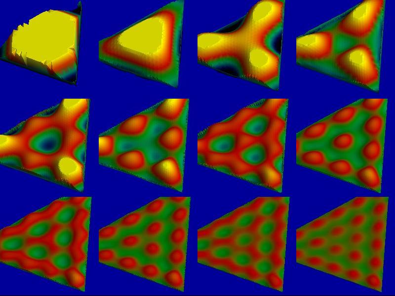
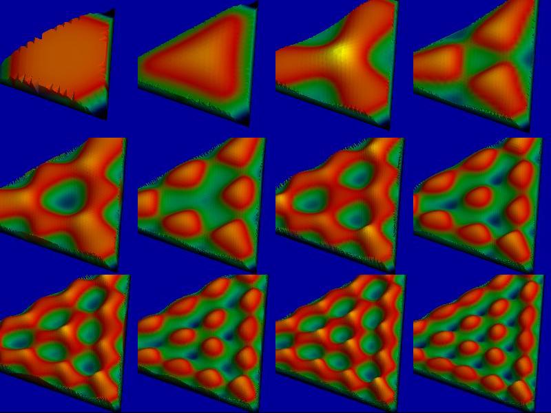
The panels of Fig. 1 plot , showing a sequence of sections of constant Fig. 2 shows the analogous plots for The -coordinates in the plot correspond to the orthogonal transverse coordinates and The function value is indicated by height and color with the color scale ranging from to for and from to for Black blue green indicates negative values and red orange yellow indicates positive values, with the zero point situated between green and red.
The triangle inequality ( and cyclic permutations) reduces to the following three conditions
| (48) | |||||
| (49) | |||||
| (50) |
Because the sum has to be even (parity condition), the only take even values. The inverse relations are
| (51) |
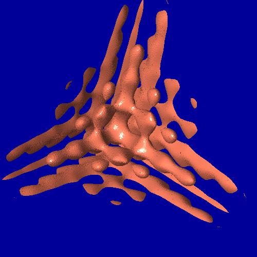
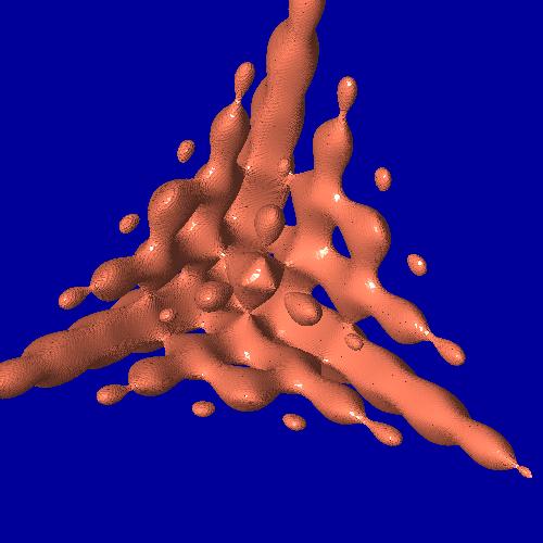
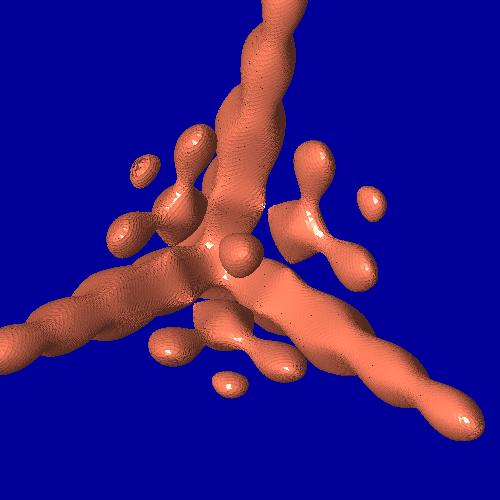
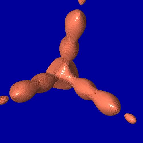
If all non-negative values of , , were allowed, the region allowed by the triangle inequality would comprise the infinite triangular pyramid in the principal octant with whose edges are the rays and the two other cyclic permutations thereof, and the faces would correspond to The extremely elongated triangles with one much smaller than the other two are situated in the immediate neighborhood of these edges. It is these configurations that give rise to the logarithmic divergence previously mentioned and contribute the bulk of the statistical weight, in a way which we will characterize more quantitatively later on. Because the lowest observable multipole starts at the edges are slightly truncated by the intersecting planes Fig. 1 shows 16 sections of constant . The most negative values of occur near the edges. In the central region we observe a sequence of acoustic oscillations. First, we observe a single maximum situation at the center of the triangle (corresponding to an exactly equilateral configuration). The center oscillates back down but three new maxima appear situated between the centre and the vertices. The process repeats itself, so that the number of local maxima progresses according to the sequence [An animation of a sequence more finely sampled is available at http://www.apc.univ-paris7.fr/bucher/bispectrum.]
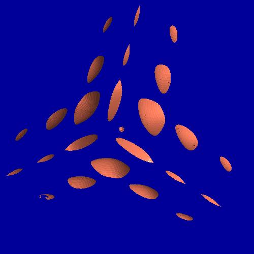
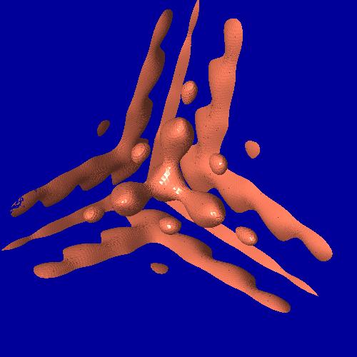
In Figs. 3 and 4 we show isosurfaces of the function at values -10, -4, -2, +2, +4, +10. The domain is an infinite triangular pyramid in the first octant and in the first panel all the isosurfaces for this most negative value terminate on the boundary. The long curved lens-like structures are situated along the edges and track the acoustic oscillations of the two-point power spectrum, as discussed in more detail below. As the threshold isovalue is increased, new bubbles appear and coalesce. The null isosurface is not shown because it has a regular Swiss cheese appearance, so that it is impossible to see inside.
The TTT reduced bispectrum is given by Komatsu & Spergel (2001)
| (55) | |||||
where the primordial power spectrum for the gravitational potential is defined by
| (56) |
and the local ansatz (4) is assumed. is the CMB transfer function (computed with a Boltzmann solver, here using CAMB). At the same time the expectation value for the CMB power spectrum is given by
| (57) |
If we assume a simple power spectrum (e.g., exact scale invariance or a homogeneous power law), its contribution to the reduced bispectrum is featureless and does not single out any special scales. However the CMB transfer function contains interesting physics characterized by a variety of scales (e.g., the scale of matter-radiation equality, horizon size at last scattering, the shape of the visibility function, etc.) and it is these features, which are presumably well understood, that should be helpful in distinguishing a primordial bispectrum from other contaminants.
We re-examine some of the arguments previously put forth by exploiting the approximate integral for the statistical information in eqn. (25) in light of the exact local bispectrum and exact inner product for a particular experiment (here taken to be the PLANCK instrument using an uncontaminated CMB map obtained by combining in quadrature the 100, 143, and 217 GHz channels with the specifications published in the PLANCK bluebook (Planck Collaboration, 2006)).
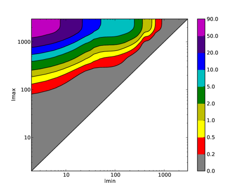
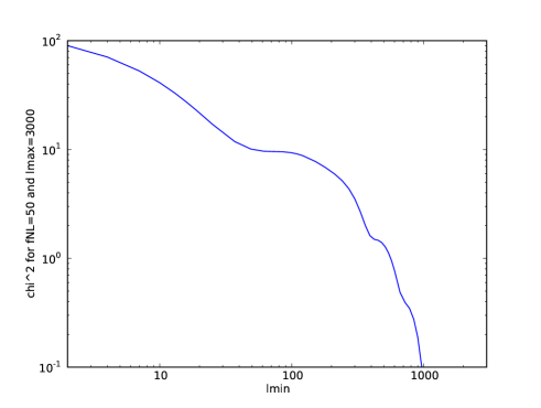
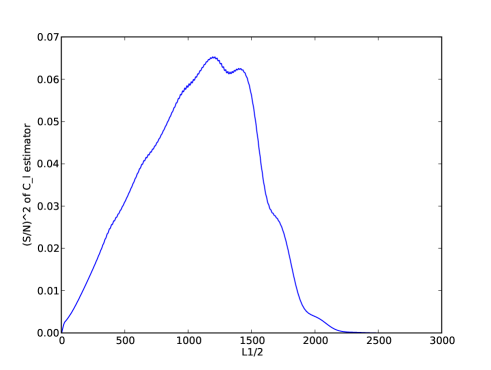
In order to visualize how the statistical weight of the signal is distributed in space, it is useful to make various cuts and integrate taking into account these cuts. (We take as that is roughly the order of magnitude of the central value of the WMAP5 results.) The simplest cuts one can make is to restrict the multipole values to lie in a range . The resulting as a function of and is shown in Fig. 5. We observe that almost all the statistical weight comes from the coupling of the lowest with the largest .
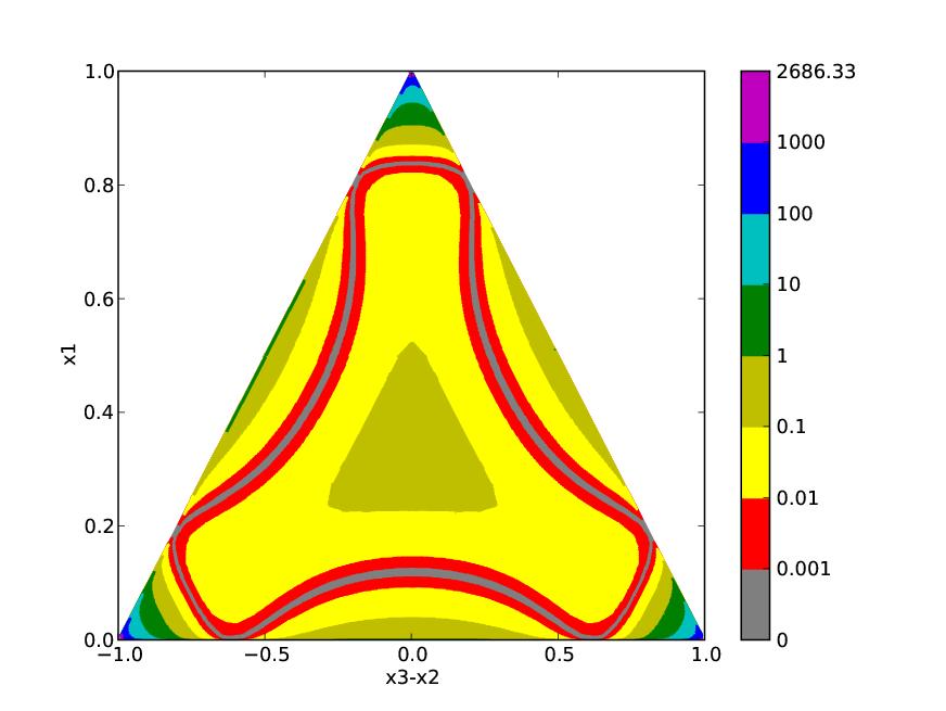
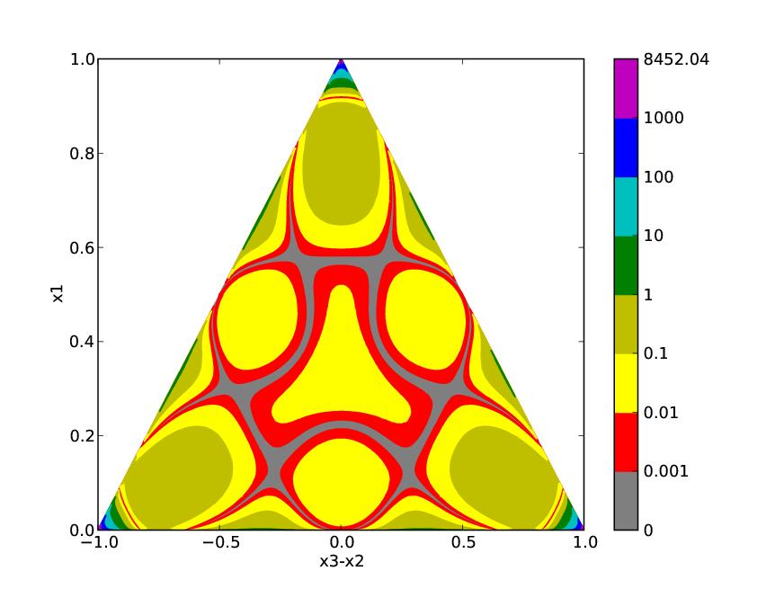
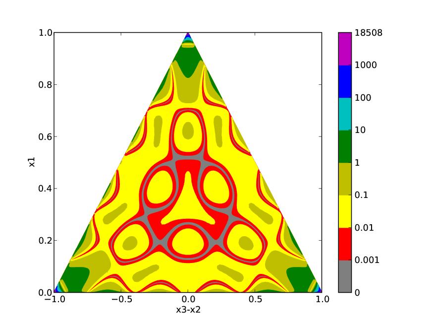
It is useful to adopt the following parameterization under which there is one dimensionful quantity and a number of redundant dimensionless quantities (of which only two are linearly independent). For our dimensionful quantity we choose . The dimensionless shape of the triangle in harmonic space is characterized by
| (58) |
where and are as defined in eqn. (50). The quadruplet provides a redundant set of coordinates (satisfying ) and the triangle inequality is satisfied if and only if and The three edges of the allowed region are defined by and and where
Fig. 6 shows the weights (the sum over of which corresponds to the ) for three different slices with fixed at 1000, 2000, 3000, respectively. Since the absolute value of the weights on such a slice is not very meaningful, they have been divided by the average value on the slice. In other words, values smaller than unity correspond to regions with lower than average weight, and values larger than unity to regions with higher than average weight. The preponderance of the extreme configurations around the vertices is manifest in this figure, although their integrated contribution is not so easy to see.
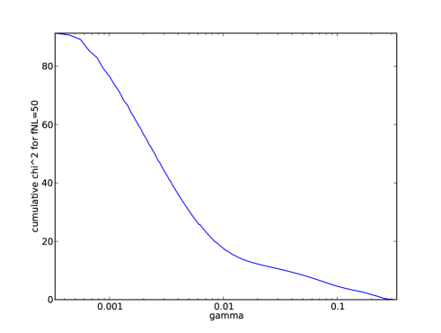
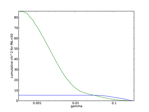
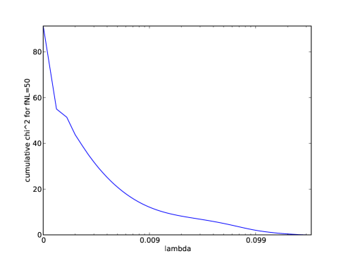
We now define two families of cuts in order to quantify how much the triangles of the central region contribute to the total integrated signal. Firstly we may define a family of expanding concentric equilateral triangles parameterized by according to the relation with This is one way to cut out nearly flattened or collinear triangles. Secondly, we may cut away at the corners by requiring that where so that the triangular region becomes hexagonal. The results of the integrated for for these two families of cuts is indicated in Fig. 7. In the second panel the integrated contributions for positive and negative values of the bispectrum are examined separately. We observe that the exploitable signal is heavily concentrated in the corners and very little statistically useful signal is present where the bispectrum is actually changing sign.
4 Prospects for detecting acoustic oscillations from vertex configurations
In the previous section we investigated the imprint of physics occurring around the time of recombination on the bispectrum, which intuitively may be characterized by departures from a constant function of the bispectral ratio defined in (46). We observed a rich pattern of acoustic oscillations in the -plane as varies. However unfortunately, the statistical weight of this central region is negligible, at least for an experiment like PLANCK given the limits on set by WMAP. For PLANCK there is simply not enough signal-to-noise in this region, as we have seen, although there may be some hope with a next-generation satellite experiment such as some of the most ambitious proposals for a B-polarization satellite.
The remaining window for detecting bispectral oscillations resides in the -dependence of in extreme vertex configurations. These configurations are defined by , which automatically means that because of the triangle inequality. Hence we define and . Using definition (47), in this limit can be written as
| (59) | |||||
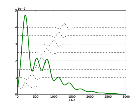
Here we have used the fact (shown numerically) that for these squeezed triangle configurations is practically constant as a function of . We conclude that in the squeezed limit the bispectrum is proportional to the power spectrum as a function of . This is shown explicitly in Fig. 8. [Alternatively, in a description that keeps the 3 different multipoles explicitly, one can use the defined in (50). Then the squeezed configuration corresponds with , the prefactor in (59) depends on and only, and we have a power spectrum behaviour as a function of .]
To explain why does not depend on in the squeezed limit, we start from the integral expression (55) for the bispectrum . In this limit the dominant contribution to the integral is proportional to
| (60) | |||
| (61) | |||
| (62) |
where for clarity we insert an exactly scale invariant power spectrum, with but all the arguments carry over to approximately scale invariant spectra. The dominant contribution to the radial integral in the last line occurs at , where is the radius of the surface of last scatter, and the dominant values of the radial wave number are situated around The first spherical Bessel function varies slowly while the the last two oscillate rapidly. This causes the integral to cancel except near the resonance, where is very nearly equal to modulo a negligible offset of approximately We therefore approximate eqn. (62) by
| (65) | |||||
| (66) | |||||
| (67) |
So we recover the fact that the bispectrum is proportional to the power spectrum as a function of , times a prefactor that only depends on . We have confirmed by numerical integration of the exact expression that the factorization on the last line is a good approximation when is much less than the scales of the power spectrum acoustic oscillations and the damping. This factorization property greatly simplifies constructing estimators in the vertex region by reducing the feature detection problem to essentially a one-dimensional problem.
We construct filters to detect the presence of several peaks and troughs in the bispectrum at positions corresponding to the peaks and troughs of the two-point power spectrum, which is of course now well known experimentally. The mathematical problem of how best to construct these filters is not completely well-defined, so there is some arbitrariness in the choice of filters designed to pick up the various features. Nevertheless other filter choices can be expected to yield results differing only slightly. We first describe our filter templates as if they were acting on the two-point power spectrum and then indicate how to carry over these templates to the bispectrum problem, which is essentially a question of how to deal with the two additional transverse dimensions.
We define the absence of features as the constancy of and construct two types of filters. The first takes a discretized second derivative of the power spectrum and is used to detect the peaks and troughs. We require this filter to give zero for a linear rise or fall in . The second filter evaluates a discretized first derivative in order to detect a rise or fall in .
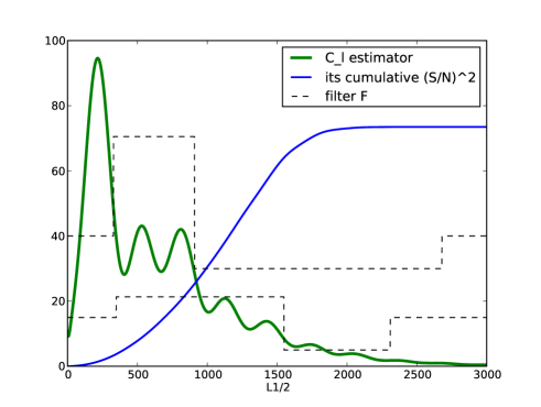
The first filter type evaluates an integral over some window function times the second derivative of , where the support of the window function for a peak, for example, would extend approximately from the trough on the left to the trough on the right. This is the optimal width because making the filter narrower would decrease the signal-to-noise by relying on too few noisy data points and a broader filter would bring in cancellations from neighboring regions of opposite sign, likewise diminishing the signal-to-noise. One candidate for the second-derivative filter would use the second derivative of a Gaussian profile, but this choice has the drawback of an infinite support, which would have to be cut off. Here we use instead a piecewise linear filter profile. For the first-derivative filter we use a step function constantly positive to the left of a certain value of and constantly negative to the right. The central value, the width to the left, and the width to the right are the three parameters in this filter. The relative heights of the left-hand and right-hand sides are fixed by the constraint that the integral of the filter should be zero. The profiles used are shown in Fig. 8 in relation to the predicted signal.
For the implementation in -space, we include only Going any higher would only marginally improve the signal and would tend to smooth the power spectrum. Then we group together triplets with the same . The function from the factorization in eqn. (67) is found numerically and with each such group the best estimator for (the expectation value of which is ) is constructed. The estimators for each triplet are combined according to inverse variance weighting. Explicitly, the resulting estimator is given by (using the more precise notation instead of )
| (68) |
where as before and the sum is over the two directions transverse to , i.e. and , under the condition that . Here is the normalization of the inverse variance weights, given by
| (69) |
This estimator and its signal-to-noise ratio squared for the case of an detection are shown in Fig. 8. It represents one way of going beyond the single number to describe the bispectrum (see also Munshi & Heavens (2009)).
To look for specific features, the estimator is summed with respect to the filters described above. The resulting statistic is given by
| (70) |
The variance of is given by
| (71) |
The signal-to-noise ratios of this estimator in the case of are given in Table 1. Once more we have assumed the three Planck channels at 100, 143, and 217 GHz, and we have used . For an arbitrary the table entries in the last column should be multiplied by a factor of .
| Feature | Center | |||
| 1st peak | 210 | 100 | 170 | 0.43 |
| 1st trough | 400 | 130 | 130 | 0.69 |
| 2nd peak | 530 | 100 | 120 | 0.19 |
| 2nd trough | 660 | 100 | 120 | 0.27 |
| 3rd peak | 810 | 130 | 160 | 0.70 |
| 3rd trough | 1010 | 140 | 120 | 1.08 |
| 4th peak | 1140 | 110 | 120 | 0.34 |
| 4th trough | 1300 | 130 | 120 | 0.53 |
| Drop A | 910 | 580 | 1770 | 11.3 |
| Drop B | 1550 | 1200 | 760 | 21.9 |
5 Binned bispectral estimator implementation
In this section we describe how to estimate from a CMB map having been provided the details of the CMB experiment (instrument noise, beam profile, …) and a theoretical model, from which we require the primordial power spectrum and transfer functions . As explained in a previous section, we need to evaluate the binned approximation to the ideal estimator (21) or to some variant (29). We can write the binned estimator as
| (72) |
with the binned weights given by
| (73) |
Since we have changed the sum over into a sum over , we have to divide the weights by 2 (or 6) in the case where 2 (or 3) bins are equal, to avoid overcounting.
Computing this estimator involves four distinct steps:
-
1.
Computing the theoretical bispectrum ;
-
2.
Deriving the binned weights from it;
-
3.
Computing the binned bispectrum from the map;
-
4.
Combining the above to yield (or another estimator).
The modular code we developed follows these 4 steps and the results from each step are saved separately. Hence step 3, for example, is completely independent of steps 1 and 2, so that when trying out another mask, say, only the code corresponding to steps 3 and 4 has to be rerun. While we focus in this section on , the modular setup of the code makes it very easy to compute another bispectral quantity instead. For example, by replacing in step 2 the -weights defined above by the binned version of the weights defined in (70), we can compute the statistic to detect acoustic bispectrum features.
5.1 Implementation notes
After getting the transfer functions from CAMB, to save computing time in step 1, eqn. (55) for the reduced bispectrum is not evaluated for all -triplets, but only for a representative (large) number. The other necessary values are determined by 3D linear interpolation. Our code also allows for the use of a 3D cubic interpolation scheme, but for the large number of exact “grid points” used we found no significant increase in accuracy compared to the linear scheme, which is faster and already very accurate.
To compute the weight for a bin in step 2 one can either evaluate all terms inside the bin and sum them explicitly or, much faster, for large bins use a simple 3D integration scheme (here based on tetrahedronisation of the bin-cubes). Both methods are implemented in our code. In the first case all the values of , , and are pre-computed and saved to speed up any consequent calculations for the same cosmological model (at the cost of additional memory usage). However, because of the slow variation of , the second (approximate) method is highly accurate and due to its higher speed and lower memory usage generally to be preferred.
Computing the binned observed bispectrum in step 3 involves multiplying the observed with the inverse beam and window function operators, applying the masks (if any), and determining the maximally filtered maps according to (9). However, it is in this step that binning is a necessary ingredient to reduce computing time, so instead of computing the maximally filtered maps for each individual , they are only computed per bin, producing . Finally the binned observed bispectrum is computed using the binned analogue of eqn. (8). Healpix (Gorski et al., 2005) is used to carry out the spherical harmonic transforms.
Using the files with the results from steps 2 and 3 it is simple and quick to evaluate in step 4 the sum (72) and find the result for . Its variance is also computed. In the case of multiple maps (different realizations of the same CMB sky) the result is computed in a number of different ways to check consistency: by first combining the different bins to find a result per map, and then combining the different maps; or by first combining the maps to find an averaged result per bin, and then combining the bins. Moreover, using the set of maps we can also compute an observed variance and use that in the weights instead of the theoretical variance. In particular this allows us to see the effects of deviations from Gaussianity in the variance, which become important when is several standard deviations away from zero for the experiment under consideration.
Steps 2 and 4 are fast (about 10 minutes and 10 seconds, respectively, on a laptop with an Intel Core 2 Duo P8400 processor (using only one core)), while step 1 is slower (about 1.5 hours), all for . If necessary, step 1 can be made faster by sampling the (at present probably unnecessarily densely sampled) theoretical bispectrum more sparsely. Step 3 is the slowest, taking about 45 minutes for one map with and Healpix parameter . However, we have parallelized this step, so that multiple maps can be run in parallel, and further code optimizations are in progress. We run this code on a blade server with 16 quad-core Intel Xeon 5345 processors on 8 blades (64 cores in total with 4 GB of memory per core; one core of these performs roughly the same as a core of the P8400 mentioned above), so that a set of 100 maps takes about 1.5 hours.
5.2 Binning scheme
To run our code we have to specify a binning scheme. We choose a divisional scheme, although other schemes are implemented as well. This means that we first split the interval into two at the intermediate value , where the parameter lies between 0 and 1. Next each of these intervals is split into two again using parameters and , each rescaled to lie between 0 and 1. This process can be repeated as many times as necessary.
We can quantify how much the variance increases due to binning, compared with an ideal estimator without binning, using the parameter defined in (30). The results are summarized in Table 2. To find the maximum value of we have varied the 7 parameters , , , , , , and (only 3 parameters for the case of 4 bins, and for the cases of 16 to 64 bins the remaining divisional parameters have been fixed at 0.5) on a fixed grid and assumed (as well as the noise and beam characteristics of the Planck 100 GHz channel). We see that using 64 bins instead of all the 1999 -values in the interval gives an immense reduction of computing time at the cost of only a increase in the variance. Even smaller numbers of bins still give a quite acceptable increase of variance.
As an explicit example, the maximum value of for 64 bins was reached for the following parameter values: , , and . This corresponds to the following bin separator values for : (2, 3, 5, 7, 9, 11, 13, 15, 17, 25, 33, 41, 49, 57, 65, 73, 81, 101, 121, 141, 161, 181, 201, 221, 241, 261, 281, 301, 321, 341, 361, 381, 401, 441, 481, 521, 561, 601, 641, 681, 721, 761, 801, 841, 881, 921, 961, 1001, 1040, 1088, 1136, 1184, 1232, 1280, 1328, 1376, 1424, 1496, 1568, 1640, 1712, 1784, 1856, 1928, 2000).
| Number bins | Overlap () |
|---|---|
| 4 | 0.608 |
| 8 | 0.846 |
| 16 | 0.925 |
| 32 | 0.974 |
| 64 | 0.993 |
5.3 Validation of estimator
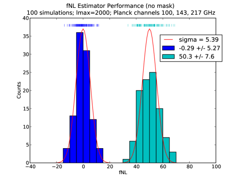
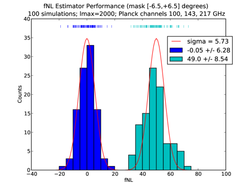
To test our binned estimator, we applied it to 100 CMB-only maps with and , kindly provided by Michele Liguori based on the WMAP5-only best-fit parameters (Liguori et al., 2007). To these maps we added the effects of uniform white noise and a Gaussian beam according to the specifications of the 100, 143, and 217 GHz channels of the Planck experiment (combined in quadrature) (Planck Collaboration, 2006). We have used 64 bins, with divisional parameters such that is maximal.
The results can be found in Fig. 9. Without a mask, we recover for a value of and for of . These results agree with those obtained with the KSW estimator. We also tested with a simple band mask of degrees around the galactic equator and found and , respectively. Here the masked area was filled with the average of the rest of the map and any remaining monopole was subtracted. A more detailed study of the influence of masks and how to treat them will be the subject of a future publication.
The smooth curve in both plots is the predicted Gaussian distribution based on the calculated theoretical variance when nonlinear corrections are ignored. Its standard deviation is without a mask and with the band mask. The modest increase with the mask is due to the decreased sky fraction. We see that for , which corresponds to a detection of several sigma, the actual standard deviation starts deviating from the Gaussian one as nonlinear corrections become important.
6 Discussion
The search for primordial non-Gaussianity is presently in its early stages. Non-Gaussianity of the local type is motivated by multiple-field inflation and if detected would have a substantial impact on our understanding of the physics of the early universe. At present we have only an upper limit with in the interval at 95% confidence according to the official WMAP5 analysis (Komatsu et al., 2009a), which constitutes a hint of a detection. A detection has been claimed in another analysis of the WMAP data by Yadav & Wandelt (2008), and several other alternative analyses, such as using needlets (Lan & Marinucci, 2008; Rudjord et al., 2009) or spherical Mexican hat wavelets (Curto, Martínez-González & Barreiro, 2009), have been published. See also Hikage (2008); Creminelli et al. (2006, 2007); Senatore, Smith & Zaldarriaga (2009); Smith, Senatore & Zaldarriaga (2009). These analyses differ in detail but are broadly consistent. Note that a confirmed detection of a primordial of order 10 would rule out the simplest single-field slow-roll inflation models.
The PLANCK space mission promises to bring about approximately an order of magnitude improvement in sensitivity to so if the present hint of a signal is confirmed, we will have an abundance of signal-to-noise at our disposal, allowing the data to be divided in many ways in order to confirm the predicted shape for the bispectrum and to exclude other non-primordial sources of parasite bispectral power.
In this paper, we demonstrated how a binned bispectrum estimator can be useful to evaluate the perfect template with a modest number of bins, so that applying the estimator is computationally extremely efficient. Compared to other implementations of the optimal estimator, which are likewise fast, the present estimator has the advantage that it can be used to apply other templates, either for or to determine other bispectral characteristics. It will be important to develop models of the expected pattern of bispectral non-Gaussianity arising from foregrounds, instrumental artifacts, and foreground subtraction residuals. Even if very approximate, such templates will be invaluable for excluding non-primordial explanations for a possible future detection. We showed how using a binned estimator one should modify the template for primordial non-Gaussianity of the local type to optimally mask the contaminants.
We also investigated how the acoustic oscillations manifest themselves in the CMB bispectrum from local primordial non-Gaussianity and in particular evaluated the signal-to-noise for detecting various features. Although a rich pattern of non-trivial acoustic oscillations occurs in the central region of triangle shape space, we found that these oscillations contribute negligibly to the total available signal-to-noise. However, the oscillations having the same shape as the power spectrum near the vertices of triangle shape space offer a much larger signal. We also investigated broader features due to the damping, and these may be seen with PLANCK if is large enough. An observation of such features in the bispectrum matching the shape of the two-point power spectrum would constitute a convincing confirmation of a first detection. The absence of a signal in other regions where none is expected also provides a powerful check against foreground and instrumental contamination.
Acknowledgments
We would like to thank Michele Liguori for kindly providing us with simulated sky maps with non-zero that were invaluable for testing and validating our estimator. We would also like to thank Michele Liguori for useful discussions. We thank David Spergel for some insightful comments on the final manuscript.
Note added: After this manuscript was submitted to astro-ph, a paper by Fergusson, Liguori and Shellard (Fergusson et al., 2010) appeared on estimation having some overlap with the ideas developed in this paper.
References
- Acquaviva et al. (2003) Acquaviva, V.; Bartolo, N.; Matarrese, S.; Riotto, A. (2003) “Second order cosmological perturbations from inflation,” Nucl. Phys. B667, 119 (astro-ph/0209156)
- Alishahiha et al. (2004) Alishahiha, M.; Silverstein, E.; Tong, D. (2004) “DBI in the sky,” Phys. Rev. D70, 123505 (hep-th/0404084)
- Amendola (2002) Amendola, L. (2002) “The dependence of cosmological parameters estimated from the microwave background on non-gaussianity,” Ap. J. 569, 595 (astro-ph:0107527)
- Arkani-Hamed et al. (2004) Arkani-Hamed, N.; Creminelli, P.; Mukohyama, S.; Zaldarriaga, M. (2004) “Ghost Inflation,” JCAP 0404, 001 (hep-th/0312100)
- Babich (2005) Babich, D (2005) “Optimal Estimation of Non-Gaussianity,” Phys. Rev. D72, 043003 (astro-ph/0503375)
- Babich et al. (2004) Babich, D.; Creminelli, P.; Zaldarriaga, M. (2004) “The Shape of Non-Gaussianities,” JCAP 0408, 009 (astro-ph/0405356)
- Babich & Zaldarriaga (2004) Babich, D.; Zaldarriaga, M. (2004) “Primordial Bispectrum Information from CMB Polarization,” Phys. Rev. D70, 083005 (astro-ph/0408455)
- Bernardeau et al. (2002) Bernardeau, F.; Colombi, S.; Gatztanaga, E.; Scoccimarro, R. (2002) “Large-Scale Structure of the Universe and Cosmological Perturbation Theory,” Phys. Repts. 367, 1 (astro-ph/0112551)
- Bartolo, Matarrese & Riotto (2002) Bartolo, A.; Matarrese, S.; Riotto, A. (2002) “Non-gaussianity from inflation,” Phys. Rev. D65, 103505 (hep-ph/0112261)
- Bartolo, Komatsu, Matarrese & Riotto (2004) Bartolo, N.; Komatsu, E.; Matarrese, S.; Riotto, A. (2004) “Non-Gaussianity from inflation: theory and observations,” Phys. Repts. 402, 103 (astro-ph/0406398)
- Bartolo, Matarrese & Riotto (2004) Bartolo, N.; Matarrese, S.; Riotto, A. (2004) “On non-Gaussianity in the curvaton scenario,” Phys. Rev. D69, 043503 (hep-ph/0309033)
- Bartolo, Matarrese & Riotto (2004) Bartolo, N.; Matarrese, S.; Riotto, A. (2004) “Evolution of Second-Order Cosmological Perturbations and Non-Gaussianity,” JCAP 0401, 003 (astro-ph/0309692)
- Bartolo & Riotto (2008) Bartolo, N.; Riotto, A. (2008) “On the Non-Gaussianity from Recombination,” (astro-ph/08114584)
- Byrnes et al. (2008) Byrnes, C.T.; Choi, K.Y.; Hall, L.M.H. (2008) “Conditions for large non-Gaussianity in two-field slow-roll inflation,” JCAP 0810, 008 (astro-ph/08071101)
- Byrnes et al. (2009) Byrnes, C.T.; Choi, K.Y.; Hall, L.M.H. (2009) “Large non-Gaussianity from two-component hybrid inflation,” JCAP 0902, 017 (astro-ph/08120807)
- Carvalho (2009) Carvalho, C.S. (2009) “Modelling non-Gaussianity from foreground contaminants,” J. Phys. Conf. Ser. 189, 012006 (astro-ph/09013613)
- Cabella et al. (2009) Cabella, P.; Pietrobon, D.; Veneziani, M.; Balbi, A.; Crittenden, R. de Gasperis, G.; Quercellini, G.; Vittorio, N. (2009) “Foreground influence on primordial non-Gaussianity estimates: needlet analysis of WMAP5-year data,” (astro-ph/09104362)
- Cheung et al. (2008) Cheung, C.; Fitzpatrick,A.L.; Kaplan, J.; Senatore L. (2008) “On the consistency relation of the 3-point function in single-field inflation,” JCAP 0802, 021 (hep-th/07090295)
- Creminelli et al. (2006) Creminelli, P.; Nicolis, A.; Senatore, L.; Tegmark, M.; Zaldarriaga, M. (2006) “Limits on non-gaussianities from WMAP data,” JCAP 0605, 004 (astro-ph/0509029)
- Creminelli et al. (2007) Creminelli, P.; Senatore, L.; Zaldarriaga, M.; Tegmark, M. (2007) “Limits on parameters from WMAP 3yr data,” JCAP 0703, 005 (astro-ph/0610600)
- Creminelli, Senatore & Zaldariaga (2007) Creminelli, P.; Senatore, L.; Zaldarriaga, M. (2007) “Estimators for local non-Gaussianities,” JCAP 0703, 019 (astro-ph/0606001)
- Creminelli & Zaldarriaga (2004a) Creminelli, P.; Zaldarriaga, M. (2004) “CMB 3-point functions generated by non-linearities at recombination,” Phys.Rev.D70, 083532 (astro-ph/0405428)
- Creminelli & Zaldarriaga (2004b) Creminelli, P.; Zaldarriaga, M. (2004) “Single field consistency relation for the 3-point function,” JCAP 0410, 006 (astro-ph/0407059)
- Curto, Martínez-González & Barreiro (2009) Curto, A.; Martínez-González , E.; Barreiro, R.B. (2009) “Improved constraints on primordial non-Gaussianity for the Wilkinson Microwave Anisotropy Probe,” (astro-ph/09021523)
- Donzelli et al. (2009) Donzelli, S; Hansen, F; Liguori, M; Maino, D (2009) “Impact of the 1/f noise and the asymmetric beam on non-Gaussianity searches with Planck,” (astro-ph/09074650)
- Fergusson & Shellard (2007) Fergusson, J.R.; Shellard, E.P.S. (2007) “Primordial non-Gaussianity and the CMB bispectrum,” Phys. Rev. D76, 083523 (astro-ph/0612713)
- Fergusson & Shellard (2009) Fergusson, J.R.; Shellard, E.P.S. (2009) “The shape of primordial non-Gaussianity and the CMB bispectrum,” Phys. Rev. D80, 043510 (astro-ph/0812.3413)
- Fergusson et al. (2010) Fergusson, J.R.; Liguori, M.; Shellard, E.P.S. (2010) “General CMB and Primordial Bispectrum Estimation I: Mode Expansion, Map-Making and Measures of ,” (astro-ph/0912.5516)
- Gorski et al. (2005) Gorski, K.M.; Hivon, Eric; Banday, A.J.; Wandelt, B.D.; Hansen, F.K.; Reinecke, M.; Bartelman M. (2005) “HEALPix: A Framework for high resolution discretization and fast analysis of data distributed on the sphere,” Ap. J. 622, 759 (astro-ph/0409513)
- Green et al (2009) Green, D.; Horn, B.; Senatore, L.; Silverstein, E. (2009) “Trapped Inflation,” (hep-th/09021006)
- Goldberg & Spergel (2008) Gold, B. et al. (2008) “Five-year Wilkinson Microwave Anisotropy Probe (WMAP) Observations: Galactic Foreground Emission,” (arXiv:08030715)
- Goldberg & Spergel (1999) Goldberg, D.M.; Spergel, D.N. (1999) “The Microwave Background Bispectrum, Paper II: A Probe of the Low Redshift Universe,” Phys. Rev. D., 59, 103002 (astro-ph/9811251)
- Heavens (1998) Heavens, A. (1998) “Estimating non-Gaussianity in the microwave background” MNRAS 299, 805
- Hikage (2008) Hikage, C; Matsubara, T; Coles, P; Liguori, M; Hansen, F; Matarrese, S (2008) “Limits on Primordial Non-Gaussianity from Minkowski Functionals of the WMAP Temperature Anisotropies,” MNRAS 389, 1439 (astro-ph/08023677)
- Holman & Tolley (2008) Holman, R.; Tolley, A.J. (2008) “Enhanced Non-Gaussianity from Excited Initial States,” JCAP 0805, 001, (hep-th/07101302)
- Hanson et al. (2009) Hanson, D.; Smith, K.M.; Challinor, A.; Liguori, M. (2009) “CMB lensing and primordial non-Gaussianity,” (astro-ph/09054732)
- Huang (2009) Huang, Q.G. (2009) “A geometric description of the non-Gaussianity generated at the end of multi-field inflation,” JCAP 0906, 035, (hep-th/0904.2649)
- Komatsu & Spergel (2001) Komatsu, E.; Spergel, David N. (2001) “Acoustic signatures in the primary microwave background bispectrum,” Phys. Rev. D63, 063002 (astro-ph/0005036)
- Komatsu et al. (2003) Komatsu, E. et al. (2003) “First Year Wilkinson Microwave Anisotropy Probe (WMAP) Observations: Tests of Gaussianity,” ApJS 148, 119
- Komatsu et al. (2005) Komatsu, E.; Spergel, D.; Wandelt, B. (2005) “Measuring primordial non-Gaussianity in the cosmic microwave background,” Astrophys. J. 634, 14 (astro-ph/0305189)
- Komatsu et al. (2009a) Komatsu E., et al. (2009) “Five-Year Wilkinson Microwave Anisotropy Probe (WMAP) Observations: Cosmological Interpretation,” ApJS 180, 330
- Komatsu et al. (2009b) Komatsu, E. et al. (2009) “Non-Gaussianity as a Probe of the Physics of the Primordial Universe and the Astrophysics of the Low Redshift Universe,” (astro-ph/09024759)
- Lan & Marinucci (2008) Lan, X.; Marinucci, D. (2008) “The needlet bispectrum,” Electronic Journal of Statistics, 2, 332 (astro-ph/08024020)
- Liguori et al. (2007) Liguori, M; Yadav, A; Hansen, F; Komatsu, E; Matarrese, S; Wandelt, B (2007) “Temperature and Polarization CMB Maps from Primordial Non-Gaussianities of the Local Type,” Phys. Rev. D76, 105016, [Erratum-ibid. D77, 029902 (2008)] (astro-ph/07083786)
- Lyth, Ungarelli & Wands (2003) Lyth, D.H.; Ungarelli, C.; Wands, D. (2003) “The primordial density perturbation in the curvaton scenario,” Phys. Rev. D67, 023503 (astro-ph/0208055)
- Maldacena (2003) Maldacena, Juan Martin (2003) “Non-Gaussian features of primordial fluctuations in single field inflationary models,” JHEP 05, 013 (astro-ph/0210603)
- Mangilli & Verde (2009) Mangilli, A.; Verde, L. (2009) “Non-Gaussianity and the CMB Bispectrum: confusion between Primordial and Lensing-Rees Sciama contribution?,” Phys. Rev. D80, 123007 (astro-ph/0906.2317)
- Munshi & Heavens (2009) Munshi, D; Heavens; A (2009) “A New Approach to Probing Primordial Non-Gaussianity,” (astro-ph/09044478)
- Munshi et al. (2009) Munshi, D; Valageas, P; Cooray, A; Heavens, A (2009) “Secondary non-Gaussianity and Cross-Correlation Analysis,” (astro-ph/09073229)
- Naruko & Sasaki (2009) Naruko, A.; Sasaki, M. (2009) “Large non-Gaussianity from multi-brid inflation,” Prog. Theor. Phys. 121, 193 (astro-ph/08070180)
- Nitta et al. (2009) Nitta, D.; Komatsu, E.; Bartolo, N.; Matarrese, S.; Riotto, A. (2009) “CMB anisotropies at second order III: bispectrum from products of the first-order perturbations,” JCAP 0905, 014 (astro-ph/0903.0894)
- Pietrobon et al. (2008) Pietrobon et al. (2008) “Constraints on primordial non-Gaussianity from a needlet analysis of the WMAP-5 data,” (astro-ph/08122478)
- Planck Collaboration (2006) Planck Collaboration (2006) “The Scientific Programme of Planck,” (known as the Bluebook) (astro-ph/0604069)
- Pyne & Carroll (1996) Pyne, T.; Carroll, S.M. (1996) “Higher-Order Gravitational Perturbations of the Cosmic Microwave Background,” Phys. Rev. D53, 2920 (astro-ph/9510041)
- Rigopoulos, Shellard & Van Tent (2005) Rigopoulos, G.I.; Shellard, E.P.S.; Van Tent, B.J.W. (2005) “A simple route to non-Gaussianity in inflation,” Phys. Rev. D72, 083507 (astro-ph/0410486)
- Rigopoulos, Shellard & Van Tent (2006) Rigopoulos, G.I.; Shellard, E.P.S.; Van Tent, B.J.W. (2006) “Large non-Gaussianity in Multiple-Field Inflation,” Phys. Rev. D73, 083522 (astro-ph/0506704)
- Rigopoulos, Shellard & Van Tent (2007) Rigopoulos, G.I.; Shellard, E.P.S.; Van Tent, B.J.W. (2007) “Quantitative bispectra from multifield inflation,” Phys. Rev. D76, 083512 (astro-ph/0511041)
- Rudjord et al. (2009) Rudjord, O.; Hansen, F.K.; Lan, X.; Liguori, M.; Marinucci, D.; Matarrese, S. (2009) “An Estimate of the Primordial Non-Gaussianity Parameter Using the Needlet Bispectrum from WMAP,” Ap. J. 701, 369 (astro-ph/09013154)
- Santos et al. (2003) Santos, M et al., (2003) “Multiple Methods for Estimating the Bispectrum of the Cosmic Microwave Background with Application to the MAXIMA Data,” MNRAS 341,623 (astro-ph/0211123)
- Senatore, Smith & Zaldarriaga (2009) Senatore, L.; Smith, K.M.; Zaldarriaga, M. (2009) “Non-Gaussianities in single field inflation and their optimal limits from the WMAP 5-year data,” (astro-ph/09053746)
- Smith & Zaldarriaga (2006) Smith, K.M.; Zaldarriaga, M. (2006) “Algorithms for bispectra: forecasting, optimal analysis, and simulation,” (astro-ph/0612571)
- Smith, Senatore & Zaldarriaga (2009) Smith, K.M.; Senatore, L.; Zaldarriaga, M. (2009) “Optimal limits on from WMAP 5-year data,” JCAP 0909, 006 (astro-ph/09012572)
- Verde et al. (2000) Verde, L.; Wang, L.; Heavens, A.F.; Kamionkowski, M. (2000) “Large-scale structure, the cosmic microwave background, and primordial non-gaussianity,” MNRAS, 325, 412 (astro-ph/9906301)
- Yadav et al. (2008) Yadav, A.P.S.; Komatsu, E.; Wandelt, B.D.; Liguori, M.; Hansen, F.K.; Matarrese, S. (2008) “Fast Estimator of Primordial Non-Gaussianity from Temperature and Polarization Anisotropies in the Cosmic Microwave Background II: Partial Sky Coverage and Inhomogeneous Noise,” Astrophys.J.678 578 (astro-ph/07114933)
- Yadav & Wandelt (2008) Yadav, Amit P.S.; Wandelt, Benjamin D. (2008) “Evidence of Primordial Non-Gaussianity in the Wilkinson Microwave Anisotropy Probe 3-Year Data at 2.8,” Phys. Rev. Lett. 100, 181301 (astro-ph/07121148)