We consider loop observables in gauged Wess-Zumino-Witten models, and study the action of renormalization group flows on them. In the WZW model based on a compact Lie group $G$, we analyze at the classical level how the space of renormalizable defects is reduced upon the imposition of global and affine symmetries. We identify families of loop observables which are invariant with respect to an affine symmetry corresponding to a subgroup $H$ of $G$, and show that they descend to gauge-invariant defects in the gauged model based on $G/H$. We study the flows acting on these families perturbatively, and quantize the fixed points of the flows exactly. From their action on boundary states, we present a derivation of the “generalized Affleck-Ludwig rule”, which describes a large class of boundary renormalization group flows in rational conformal field theories.

1 Introduction and summary of results

Two-dimensional field theories have a rich set of interesting loop observables, much richer than in higher dimensions. The loop operators of $2D$ conformal field theories (CFT’s), in particular, whose study was pioneered by Bazhanov, Lukyanov and Zamolodchikov [1, 2, 3], have attracted considerable attention. Some of these operators describe interesting condensed-matter systems [4, 5, 6]. They have furthermore proved to be powerful tools for organizing boundary renormalization-group flows [7, 8, 9, 10, 11, 12], and they could play a role as symmetries of string theory [13, 14, 15, 16]. A partial list of further references is [17, 18, 19, 20, 21, 22, 23, 24, 25, 26, 27, 28]. Our aim in the present work will be the study of loop operators in the largest known class of exactly-solvable conformal theories, which includes all known rational CFTs: the Goddard-Kent-Olive (GKO) coset models [29, 30].

The loops under study arise as worldlines of point-like defects, or “quantum impurities”. An impurity is characterized by a state space $V$, that we will choose to be finite-dimensional, and by a Hamiltonian ${\cal H}_{\rm imp}$ which is a ${\rm dim}(V)\times{\rm dim}(V)$ matrix. This latter depends in general on the local bulk fields, which we denote collectively by $\Phi$. The classical loop observables are given by

$${\cal O}(C)={\rm tr}_{V}\,P\,e^{i\oint_{C}ds\,{\cal H}_{\rm imp}(\Phi)}\ ,$$ (1)

where $s$ parametrizes the loop $C$, and $P$ stands for path ordering. In what follows we will mostly work on the cylinder $\mathbb{R}\times S^{1}$, and let $C$ wind once around the cylinder. Strictly-speaking, the worldline of an impurity must be time-like, in which case it cannot possibly be a loop. We may however interpret ${\cal O}(S^{1})$ in the Euclidean theory as the insertion of a (probe) defect at finite temperature. Alternatively, one may take $\mathbb{R}$ to be the time direction, and think of ${\cal O}(S^{1})$ as a fixed-time observable. Both of these interpretations are familiar from the study of the Wilson and Polyakov loops in ordinary gauge theories.

Expression (1) does not, in general, make sense after the bulk fields $\Phi$ have been quantized, because of short-distance divergences. The operators ${\cal O}(C)$ must be first regularized and then renormalized, and this induces a flow in the space of impurity Hamiltonians. Computing these renormalization-group flows is one of the central problems in the subject. The fixed-point operators can often be found exactly by algebraic methods (see e.g. [17, 18, 20, 10]), while in special situations (and for specific renormalization schemes) the full flow may be integrable. In general, however, the only available analytical tool is perturbation theory. A method to compute the RG flows for a class of loop operators in the weakly-coupled Wess-Zumino-Witten (WZW) models has been proposed in ref. [8]. The key idea is to construct the regularized and renormalized operators as elements in the enveloping algebra of the current algebra, $U(\hat{\mathfrak{g}}_{k})$, using an expansion in inverse powers of the level $k$. In this paper we will show how to extend this approach to the weakly-coupled GKO models.

The most general, renormalizable by power-counting and classically scale-invariant defects in two-dimensional $\sigma$-models depend on a number of arbitrary functions on the target manifold. It is possible to reduce this infinite parameter space by imposing extra symmetries. For a WZW model with Lie group $G$, the symmetry of the defect must be a subgroup of the affine $\widehat{G}_{\rm left}\times\widehat{G}_{\rm right}$ bulk symmetry. Our first task, in section 2 below, will be to analyze the various possible reductions. As we will see, global symmetries that act transitively on the target space, such as $G_{\rm left}$, suffice to restrict ${\cal H}_{\rm imp}$ to a finite-dimensional parameter space. However, despite this huge reduction, the renormalization of ${\cal O}(C)$ remains in general an arduous task. A further simplification occurs when we extend the invariance under $G_{\rm left}$ to the full loop group $\widehat{G}_{\rm left}$ and assume that the latter acts trivially on $V$. Defects satisfying these two properties couple only to the right-moving sector of the theory, and will be referred to as holomorphic. Their Hamiltonian is parametrized by ${\rm dim}(\mathfrak{g})$ constant hermitean matrices, $M^{a}$, and depends only on the right-moving WZW currents ${\cal J}_{-}^{a}$,

$${\cal H}_{\rm imp}=-{1\over k}\sum_{a}M^{a}{\cal J}_{-}^{a}\ .$$ (2)

We henceforth focus our attention on holomorphic defects, which can be quantized algebraically, along the lines of ref. [8]. This is a restriction of convenience, not of higher principle.

The parameter space of holomorphic defects can be further reduced by imposing invariance under a global subgroup $H_{\rm right}\subseteq G_{\rm right}$ or a loop subgroup $\widehat{H}_{\rm right}\subseteq\widehat{G}_{\rm right}$. However, while the global symmetry is manifest, the affine symmetry associated with $\widehat{H}_{\rm right}$ is a priori broken by the ultraviolet cutoff. We will nevertheless argue (but will not prove) that a $\widehat{H}_{\rm right}$-invariant subspace of parameter space is present at the quantum level. This will bring us to the main claim of this paper:

The holomorphic, $\widehat{H}_{\rm right}$-invariant defects of the WZW model with group $G\supseteq H$ can be mapped to local defects, with identical RG flows, in the gauged WZW model based on $G/H$.

Notice that in the GKO construction of the state space of the coset model, one also starts from the state space of the parent WZW model, which is then projected to ($\widehat{H}_{\rm left}\times\widehat{H}_{\rm right}$) - invariant states [29, 30, 32]. What we will show in this paper is that a similar procedure works for (a class of) impurities and for their RG flows. The result is not trivial because the gauged and ungauged WZW models are related by a non-local transformation of fields [33, 34, 35].

Let us now describe in more detail this reduction. As will be derived in section 4.2, the RG flow of holomorphic defects in the WZW model is given to leading order in $1/k$ by

$$\frac{dM^{a}}{d\,{\rm log}\epsilon}=\sum_{b,c}\frac{1}{2k}\left[M^{b},\ if^{abc}M^{c}-[M^{a},M^{b}]\right]\;+\;O({1/k^{2}})\,,$$ (3)

where $\epsilon$ is a short-distance cutoff and $f^{abc}$ are the structure constants of the group $G$. These first-order equations describe a gradient flow, i.e. their right-hand-side is the variation of an action (the effective open-string action of [36]):

$$S(M)\,=\,-\frac{1}{8k}\sum_{a,b}\mbox{Tr}([M^{a},M^{b}]^{2})+\frac{1}{6k}\sum_{a,b,c}if^{abc}\mbox{Tr}(M^{a}[M^{b},M^{c}])\;+\;O({1/k^{2}})\,\;.$$ (4)

This action was studied extensively by one of us [37]. Its reduction to defects with a global symmetry $H\subseteq G$ proceeds in two steps: first specify how $H$ acts on $V$, i.e. choose a representation $R$ of $H$ with ${\rm dim}(R)={\rm dim}(V)$, and then require the matrix-valued vector $M$ to be an invariant $H$-tensor. The number of free parameters, for a given $H$ and $R$, is equal to the number of trivial representations in the decomposition of $R\otimes R^{*}\otimes\mathfrak{g}$. (Here $\mathfrak{g}$ is considered as a representation of $H$, and $R^{*}$ is the conjugate of $R$.)

We will decompose the Lie algebra as $\mathfrak{g}=\mathfrak{h}\oplus\mathfrak{g}/\mathfrak{h}$ and use an orthonormal basis $\{e^{a}\}$ of $\mathfrak{g}$ compatible with this decomposition. Indices $i$,$j$,… will run over the generators of $\mathfrak{h}$, while indices $s$,$t$,… will run over generators of $\mathfrak{g}/\mathfrak{h}$. It is useful to give separate names to the $H$-invariant couplings of the corresponding currents,

$${\cal H}_{\rm imp}=-{1\over k}\sum_{a}M^{a}{\cal J}_{-}^{a}=-{1\over k}\left(\sum_{j}\Theta^{j}{\cal J}_{-}^{j}+\sum_{s}\tilde{\Theta}^{s}{\cal J}_{-}^{s}\right)\ ,$$ (5)

where $\Theta$ is an invariant tensor in $R\otimes R^{*}\otimes\mathfrak{h}$ and $\tilde{\Theta}$ an invariant tensor in $R\otimes R^{*}\otimes\mathfrak{g}/\mathfrak{h}$. If $H=G$ and $R$ is irreducible, the invariant Hamiltonian is given by $M^{a}=\lambda\,T^{a}$ with $\lambda$ real and $T^{a}$ the generators of $G$ in the representation $R$. This is the one-parameter reduction of the RG flow analyzed in ref. [8].

The above parameter space of $H$-invariant holomorphic defects is further reduced if one imposes invariance under the action of the loop group $\widehat{H}$. There is a distinguished invariant tensor $\Theta_{R}$ in $R\otimes R^{\ast}\otimes\mathfrak{h}$, namely the one whose matrix elements coincide with those of the generators of $H$ in the representation $R$, normalized with respect to the Killing form of $\mathfrak{g}$. We will show that in the classical theory, the condition of $\widehat{H}$ invariance reads:

$$\Theta=\Theta_{R}\;.$$ (6)

However, while (5) is a consistent truncation of the complete RG flow equations, the reduction (6) is in general inconsistent at higher orders in the $1/k$ expansion. We will argue that the affine symmetry is, nevertheless, preserved on a subspace ${\Sigma}(\widehat{H},R,k)$ of the space of invariant tensors, which is a (small at large $k$) deformation of the classical subspace (6). Its precise form depends on the renormalization scheme. Proving the existence of this invariant subspace at all orders in the $1/k$ expansion is an interesting open mathematical problem. Assuming that it exists, we can identify the RG flows in ${\Sigma}(\widehat{H},R,k)$ with the flows of holomorphic defects in the $G/H$ coset model.

The RG flow of a holomorphic defect can be imprinted on other defects, or on boundaries, through fusion. This has proved to be a convenient way of organizing boundary RG flows [7, 8]. Fusion is the operation that merges the parallel worldlines of two defects, so that the region in between them shrinks to zero. Similarly, a defect loop can be fused with a parallel boundary. These operations are in general singular (see ref. [13]) but for the holomorphic (though not necessarily conformal) defects studied here the fusion is smooth. The RG flows between holomorphic defects given by (3) can therefore be imprinted smoothly on boundaries or on other defects – they are in this sense universal flows.

A simple illustration is provided by the boundary Kondo flows in WZW models. These describe the screening of a boundary “spin”, $S$, whose coupling to the bulk currents is ${\cal H}_{\rm bnry}=\lambda S^{a}J^{a}$. Affleck and Ludwig formulated a general rule [38] to determine the IR fixed point of the flow, in terms of the UV fixed point and the boundary spin. This so-called “absorption-of-boundary-spin” principle, stated originally for the physically most relevant case $G=SU(2)$, can be written succintly as follows:

$${\rm dim}(S)B_{\mu}\rightarrow\sum_{\nu}\mathcal{N}_{\mu\sigma}^{\;\;\nu}B_{\nu}\ .$$ (7)

Here $\mathcal{N}_{\mu\sigma}^{\;\;\nu}$ are the fusion coefficients of the WZW model, $\sigma$ is the highest weight of the representation $S$ of ${\mathfrak{g}}$, and the $B_{\mu}$ are maximally symmetric boundaries (on which left and right currents are identified) labeled by integrable highest weights of the Kac-Moody algebra $\hat{\mathfrak{g}}_{k}$ [39]. It was shown in [8] that the Kondo flows are all imprints of the universal flows acting on holomorphic defects,

$${\rm dim}(S)\mathbbm{1}\rightarrow O_{\sigma}\ ,$$ (8)

where the UV operator on the left corresponds to an impurity with dim($V$) = dim$(S)$ and ${\cal H}_{\rm imp}=0$, while the IR operator on the right commutes with the entire affine algebra, and $O_{\sigma}$ is the quantum version of the trace of the classical monodromy. This IR operator can be constructed explicitly as an element of a completion of the enveloping algebra $U(\hat{\mathfrak{g}}_{k})$ [20] and it obeys:

$$O_{\sigma}O_{\mu}=\sum_{\nu}{\cal N}_{\sigma\mu}^{\;\;\nu}O_{\nu}\ ,\hskip 28.45274pt{\rm and}\hskip 17.07182ptO_{\nu}B_{0}=B_{\nu}\ .$$ (9)

The Affleck-Ludwig rule follows easily from the above two relations.

This rederivation of the Kondo flows has some immediate advantages. First, it shows that the $\beta$-function of the flow (7) does not depend on the UV fixed point $B_{\mu}$. Second, one can fuse the defect flow (8) with other (e.g. symmetry-breaking) boundary states to find new boundary RG flows and fixed points [10]. In particular some, but not all, of the RG flows between twisted WZW boundary states [42] can be obtained in this way. Finally, one can derive relations between different partition functions on the annulus by freely transporting a holomorphic defect from one of the boundaries to the other.

The Affleck-Ludwig rule has been generalized to GKO coset models by Fredenhagen and Schomerus [43, 44, 45]. Conformal boundaries of the $G/H$ model are labelled by pairs $[\mu,\gamma]$ of integrable weights of the Kac-Moody algebras $\hat{\mathfrak{g}}_{k}$ and $\hat{\mathfrak{h}}_{xk}$, modulo some selection and identifications (see [45] for details). Fredenhagen and Schomerus proposed the following set of boundary RG flows:

$$\sum_{\alpha,\gamma}b_{\sigma\alpha}\,\mathcal{N}_{\alpha\beta}^{(\mathfrak{h})\;\gamma}\ B_{[\mu,\gamma]}\ \rightarrow\ \sum_{\nu}\mathcal{N}_{\sigma\mu}^{(\mathfrak{g})\;\nu}\ B_{[\nu,\beta]}\ ,$$ (10)

where $\sigma$, $\mu$, $\nu$ are weights of $\hat{\mathfrak{g}}_{k}$, $\alpha$, $\beta$, $\gamma$ are weights of $\hat{\mathfrak{h}}_{xk}$, $b_{\sigma\alpha}$ are the branching coefficients of the $\mathfrak{h}$-representation of highest weight $\alpha$ in the $\mathfrak{g}$-representation of highest weight $\sigma$, and $\mathcal{N}^{(\mathfrak{h})}$ and $\mathcal{N}^{(\mathfrak{g})}$ are the fusion rules of the corresponding affine algebras. The reader can verify, as a check, that (10) reduces to (7) when $H$ is the trivial subgroup of $G$. The above generalized Affleck-Ludwig rule reproduces a large class of known RG boundary flows in minimal models and in parafermionic theories [45].

Part of our motivation for the present work was the wish to derive the flows (10) as imprints of universal defect flows, by extending the corresponding analysis of the Kondo problem. We will argue that the flows (3) restricted to the $\widehat{H}$-invariant defects account for all the boundary flows predicted by the generalized Affleck-Ludwig rule. The existence of these RG flows, at least at this leading order in $1/k$, can be established analytically. Explicit solutions of the coupled non-linear flow equations can be, of course, also obtained by numerical means.

The rest of this paper provides the arguments and the detailed calculations supporting these claims. We begin, in section 2, with a general analysis of perturbatively-renormalizable defects in the (ungauged) WZW model. We describe the reductions of parameter space when invariance under global or affine bulk symmetries are imposed on a defect. This section extends and rectifies a misleading point in the corresponding discussion of ref. [8]. Section 3 starts with a brief review of classical gauged WZW models and their quantization. We then go on to show how the holomorphic, $\widehat{H}$-invariant WZW defects are mapped to local, gauge-invariant defects of the coset model. We also discuss the relation of special enhanced-symmetry defects with classical monodromies. In section 4 we quantize the holomorphic defects in a perturbative expansion in $1/k$, using the algebraic method of ref. [8]. We derive the flow equations (3), analyze their fixed-point structure and solve them numerically in some simple examples. These examples allow to visualize the invariant subspaces on which the generalized Kondo and the Fredenhagen-Schomerus flows are defined. Finally, in section 5 we first use the enhanced symmetries of (some of) the fixed-point operators to calculate their exact quantum spectrum. This is a straightforward extension of the results of [20]. We then explain how the Fredenhagen-Schomerus flows (10) can be obtained as imprints of our universal defect-flow equations. A technical point concerning the action of the fixed-point operators in the BRST quantization of the coset model is treated separately in appendix A .

2 Symmetries of WZW defects

In this section we analyze the classical symmetries of the defect operators (1). We begin with a general discussion of defect loops and the conformal group, and then proceed to examine the WZW defects and their possible global or affine symmetries. Finally we narrow down to the holomorphic defects, which are the main focus in the rest of the paper. This section extends and clarifies in significant ways the discussion of defect symmetries of ref. [8].

2.1 Conformal, chiral and topological defects

The observables (1) are traced evolution operators for a quantum impurity moving along the trajectory $C$ and interacting locally with the fields in the bulk. The latter are for now classical, while the impurity is from the very start quantum. We are interested in impurities which are scale-invariant at the classical level, so that ${\cal H}_{\rm imp}$ contains no dimensionful couplings. Renormalization may generate couplings with the dimension of mass. These are relevant in the infrared and we will assume that they are tuned to zero.

In a four-dimensional theory scale invariance is very restrictive: it forces ${\cal H}_{\rm imp}$ to be linear in the scalar and/or the gauge fields. In two dimensions, on the other hand, there is much greater freedom. If the bulk theory is a non-linear (ungauged) $\sigma$-model with fields $\Phi$ parametrizing a target manifold ${\cal M}$, the most general classically scale-invariant defect Hamiltonian reads [8]:

$$\int_{C}ds\,{\cal H}_{\rm imp}=\int_{C}d\zeta^{\alpha}\,[\partial_{\alpha}\Phi\cdot{\mathbf{B}}(\Phi)+\epsilon_{\alpha\beta}\partial^{\beta}\Phi\cdot{\mathbf{C}}(\Phi)]\ .$$ (11)

Here $\zeta^{\alpha}$ are the coordinates of the two-dimensional spacetime, and $\epsilon_{\alpha\beta}$ is the antisymmetric tensor. ${\mathbf{B}}\cdot d\Phi$ and ${\mathbf{C}}\cdot d\Phi$ are the pull-backs on the 2D spacetime of arbitrary matrix-valued one-forms ${\mathbf{B}}$ and ${\mathbf{C}}$ on the target ${\cal M}$. There are no dimensionful parameters in ${\cal H}_{\rm imp}$ because $\Phi$ has dimension zero. It is convenient to introduce the short-hand notation

$${\cal W}_{\alpha}\,d\zeta^{\alpha}:=-i(\partial_{\alpha}\Phi\cdot{\mathbf{B}}+\epsilon_{\alpha\beta}\partial^{\beta}\Phi\cdot{\mathbf{C}})\,d\zeta^{\alpha}\ .$$ (12)

We can consider ${\cal W}$ as a (composite) matrix-valued connection form, and the loop observables ${\cal O}(C)$ as the corresponding Wilson loops. However, no assumptions about the transformation properties of ${\cal W}$ are being made at this stage. Notice for later reference that in light-cone coordinates the impurity “Hamiltonian” is   ${\cal H}_{\rm imp}=i{\cal W}_{+}\pm i{\cal W}_{-}$, according to whether $C$ is in the time or in the space direction.

The scale invariance of (11) extends to invariance under all conformal transformations which preserve the defect worldline $C$. This symmetry is further enhanced if, as a result of the field equations, ${\cal W}$ turns out to define a flat connection, i.e. if

$$\partial_{\alpha}\mathcal{W}_{\beta}-\partial_{\beta}\mathcal{W}_{\alpha}+[\mathcal{W}_{\alpha},\mathcal{W}_{\beta}]=0\ .$$ (13)

In this case the non-abelian Stokes theorem implies that ${\cal O}(C)$ is invariant under arbitrary continuous deformations of the curve $C$. Such defects are therefore topological, and on a cylindrical spacetime they define a set of dim$(V)$ conserved charges. A continuous family of such defects gives an infinite number of integrals of motion and is usually tantamount to classical integrability (see for instance [31]).

Quantization breaks, in general, the scale invariance of the defect loop even when the bulk theory is conformal. This is because the definition of ${\cal O}(C)$ requires the introduction of a short-distance cutoff. As the cutoff $\epsilon$ is removed, the coupling functions ${\mathbf{B}}(\Phi)$ and ${\mathbf{C}}(\Phi)$ flow either to infinity or to infrared fixed points where scale-invariance is restored. The fixed-point operators $O^{*}(C)$ commute with the diagonal subalgebra of the full ${\rm Vir}_{\rm left}\oplus{\rm Vir}_{\rm right}$ conformal symmetry of the bulk. More explicitly, if $\overline{L}_{n}$ and $L_{n}$ are the left- and right-moving Virasoro generators on a cylindrical spacetime, then

$$[\,L_{n}-\overline{L}_{-n}\,,\,O^{*}(S^{1})\,]\,=\,0\ \ \ \ \ \mbox{for all}\;n\in{\mathbb{Z}}\ .$$ (14)

Topological operators, first introduced in Conformal Field Theory by Petkova and Zuber [17], commute separately with ${\rm Vir}_{\rm left}$ and ${\rm Vir}_{\rm right}$. As explained for example in [19, 13], the topological defects form a small subset of the much larger class of conformal defects and they are characterized by a vanishing reflection coefficient.

A third interesting class of defects are the chiral defects, which commute with the algebra ${\rm Vir}_{\rm left}$ but not necessarily with ${\rm Vir}_{\rm right}$. Chiral defects need not be scale-invariant, but the fixed points to which they flow are always topological. The different classes of defects are summarized in table 1. Examples of chiral defects include minimal model defects perturbed by fields which are holomorphic but have fractional scaling dimension [1, 23], and defects coupling only to the right-moving currents of the WZW model [8]. In addition to ${\rm Vir}_{\rm left}$, these defects can also be shown to commute with the (closed-string) Hamiltonian on the cylinder, $L_{0}+\bar{L}_{0}$. They may thus be transported freely in the time direction. Therefore they define conserved charges and can imprint their RG flows on boundaries.

Defect type	Defining property
conformal	Commutes with ${\rm Vir}_{\rm diag}$
chiral	Commutes with ${\rm Vir}_{\rm left}$
topological	Commutes with ${\rm Vir}_{\rm left}\oplus{\rm Vir}_{\rm right}$
holomorphic	No dependence on the left-moving sector,
	hence commutes with ${\cal A}_{\rm left}$

Table 1: The four types of defects. Holomorphic defects will be defined in section 2.3. ${\rm Vir}_{\rm diag}$ is the diagonal Virasoro algebra, while ${\cal A}$ denotes the chiral algebra, with respect to which the CFT is rational. All holomorphic defects are chiral, but a chiral defect need not be holomorphic.

2.2 Global versus affine group symmetries

We specialize now to the WZW models, whose action reads [48]

$$I_{\rm WZW}=\frac{k}{16\pi}\,\int_{\Sigma}\,{\rm Tr}^{\prime}\,(\partial^{\alpha}g\,\partial_{\alpha}g^{-1})-\frac{k}{24\pi}\,\int_{\cal B}{\rm Tr}^{\prime}\,(g^{-1}\partial_{\alpha}g\,g^{-1}\partial_{\beta}g\,g^{-1}\partial_{\gamma}g)\,\epsilon^{\alpha\beta\gamma}\ ,$$ (15)

where $g$ takes values in a Lie group $G$, the level $k$ is a positive integer and ${\cal B}$ is a $3d$-manifold whose boundary is the $2d$-spacetime $\Sigma$. To avoid heavy notation, we have assumed that $G$ is simple and compact. More generally, one must choose separately the level of each simple factor of $G$. Following the conventions of [49], we have defined ${\rm Tr}^{\prime}(XY)={\rm tr}_{R}(XY)/{x}_{R}$, where $x_{R}$ is the Dynkin index of the representation $R$. The long roots of $\mathfrak{g}={\rm Lie}(G)$ will always be normalized to $\sqrt{2}$. The classical field equations imply that

$$\partial_{\pm}{\cal J}_{\mp}=0\ ,\ \ \textrm{where}\ \ {\cal J_{-}}=ik\,g^{-1}\partial_{-}g\ \ \ \textrm{ , }\ {\cal J_{+}}=ik\,g\partial_{+}g^{-1}\$$ (16)

and $\zeta^{\pm}=\zeta^{0}\pm\zeta^{1}$. These are the canonically normalized currents of the WZW model which generate the symmetry transformations $g\,\to\,\overline{\Omega}(\zeta^{+})\,g\,\Omega(\zeta^{-})^{-1}$, i.e. the loop extension of the global $G_{\rm left}\times G_{\rm right}$ symmetry of (15). We will denote the loop group by $\widehat{G}_{\rm left}\times\widehat{G}_{\rm right}$.

Consider next a generic, classically scale-invariant impurity Hamiltonian. Its associated one-form field (12) can be parametrized conveniently as follows:

$$({\cal W}_{-}\,,\,{\cal W}_{+})=(\,{\cal M}^{a}(g){\cal J}^{a}_{-}\,,\,\bar{\cal M}^{a}(g){\cal J}^{a}_{+}\,)\ ,\$$ (17)

where ${\cal M}^{a}$ and $\bar{{\cal M}}^{a}$ are ${\rm dim}(\mathfrak{g})$ independent matrix-valued functions on the group manifold, ${\cal J}^{a}_{\pm}$ are the components of the currents along the Lie-algebra direction $a$, and repeated indices are implicitly summed. The total number of independent coupling functions is therefore equal to $2\,{\rm dim}(\mathfrak{g})\times{\rm dim}(V)\times{\rm dim}(V)$. To reduce this large freedom we may impose invariance under a global subgroup $H\subseteq(G_{\rm left}\times G_{\rm right})$ of the bulk symmetry, or under its affine extension $\widehat{H}\subseteq(\widehat{G}_{\rm left}\times\widehat{G}_{\rm right})$. In either case $V$ must carry a unitary $H$-representation $R$ that describes the action of the symmetry on the defect states,

$$\Omega\in H\longrightarrow R(\Omega)\,\in\,{\rm End}(V)\ .$$ (18)

If the symmetry is affine, the action depends on the space-time position of the defect. Now the matrix elements of $Pe^{-\oint{\cal W}}$ will be invariant if and only if a transformation of the bulk field transforms ${\cal W}$ as a gauge connection:

$${\cal W}_{\alpha}\ \to\ R(\Omega)\,{\cal W}_{\alpha}\,R(\Omega)^{-1}+\,R(\Omega)\partial_{\alpha}\ R(\Omega)^{-1}\ .$$ (19)

Of course, the inhomogeneous second term is absent if we only require global symmetry. It should be stressed that ${\cal W}$ is a composite field, so its transformation is determined by that of the field $g$. Thus (19) is a restriction on the couplings ${\cal M}^{a}$ and $\bar{{\cal M}}^{a}$. As will become clear immediately, this restriction is more severe in the affine than in the global case.

Let us focus now on defects preserving the full left global symmetry, $g(\zeta^{\alpha})\to\overline{\Omega}g(\zeta^{\alpha})$ for any constant $\overline{\Omega}\in G_{\rm left}$. This is a transitive symmetry, which can be used to bring $g$ at the impurity position to any desired value. Transitive global symmetries fix all functional dependence in ${\cal H}_{\rm imp}$ and restrict the latter to a finite-dimensional parameter space. In the case at hand, the covariant Hamiltonian must be given by:

$${\cal M}^{a}(g)=-\frac{i}{k}\,\bar{R}(g)M^{a}\,\bar{R}(g^{-1})\ \ \ {\rm and}\ \ \ \ \bar{\cal M}^{a}(g)\,=\,-\frac{i}{k}\,[{\rm Adj}(g^{-1})]^{ab}\,\bar{R}(g)\,\bar{M}^{b}\,\bar{R}(g^{-1})\ ,$$ (20)

where $\bar{R}(g)$ is the WZW field in the representation $\bar{R}$ of $G_{\rm left}$ in which the impurity states transform, ${\rm Adj}(g)$ is the field in the adjoint representation, while $M^{a}$ and $\bar{M}^{a}$ are constant hermitean matrices. (A factor $1/k$ has been pulled out for later convenience.) To verify (19) one uses $\bar{R}(\overline{\Omega}g)=\bar{R}(\overline{\Omega})\bar{R}(g)$ and the simple identity

$${\cal J}^{a}_{+}\,[{\rm Adj}(g^{-1})]^{ab}=[ik\,(\partial_{+}g^{-1})g]^{b}\ .$$ (21)

Both the above expression and the right WZW currents ${\cal J}^{a}_{-}$ are invariant under global $G_{\rm left}$ transformations. It then follows immediately that impurity Hamiltonians of the form (20) are covariant under $G_{\rm left}$, as advertized.

Can we extend this symmetry to $\widehat{G}_{\rm left}$ ? The right currents are invariant, but (21) transforms inhomogeneously when $\overline{\Omega}$ is a non-constant function of $\zeta^{+}$. Inserting in the expression for ${\cal W}$ and comparing with the inhomogeneous piece in (19), we deduce that the affine left symmetry fixes $\bar{M}^{a}=\bar{T}^{a}$, where $\bar{T}^{a}$ are the normalized generators of $\mathfrak{g}$ in the representation $\bar{R}$. The matrix elements of the generators coincide with those of an invariant tensor, so that $\ [{\rm Adj}(g^{-1})]^{ab}\,\bar{R}(g)\,\bar{T}^{\,b}\,\bar{R}(g^{-1})=\bar{T}^{\,a}$. Thus the $\widehat{G}_{\rm left}$-covariant Hamiltonians take the simpler form:

$${\cal M}^{a}(g)=-\frac{i}{k}\,\bar{R}(g)M^{a}\,\bar{R}(g^{-1})\ \ \ {\rm and}\ \ \ \ \bar{\cal M}^{a}(g)=-\frac{i}{k}\,\bar{T}^{a}\ .$$ (22)

The reader can verify that any other choice for $\bar{M}^{a}$ would fail to generate the inhomogeneous piece in (19) for non-constant $\overline{\Omega}(\zeta^{+})$. Notice that the covariant Hamiltonians (20) and (22) depend on the choice of representation $\bar{R}$ for the defect states.

All $\widehat{G}_{\rm left}$-invariant defects are topological at the classical level. This follows from the field equations and the identity $\ \bar{T}^{a}{\cal J}_{+}^{a}=ik\bar{R}(g)\partial_{+}\bar{R}(g^{-1})$, which imply that the connection ${\cal W}$ given by (22) is flat for any choice of $M^{a}$. The same conclusion follows from a different argument: the loop observables of $\widehat{G}_{\rm left}$-invariant defects, ${\cal O}(C)$, have vanishing Poisson brackets with the left-moving currents which generate this symmetry. Since the left-moving component of the energy-momentum tensor ${\rm T}_{++}$ is quadratic in the left currents, its Poisson bracket with ${\cal O}(C)$ is also zero. Thus ${\cal O}(C)$ is chiral and, being conformal, it is automatically topological. Let us pause and take stock of our main conclusion so far: The $G_{\rm left}$-invariant defects of the WZW model with group $G$ are parametrized by a representation $\bar{R}$ of $G$ and by $2\,{\rm dim}(\mathfrak{g})$ hermitean matrices $M^{a},\bar{M}^{a}\in{\rm End}(V)$. For affine $\widehat{G}_{\rm left}$ invariance $\bar{M}^{a}$ must equal $\bar{T}^{a}$, the generators of $G$ in the representation $\bar{R}$.

Quantization respects the global symmetry, so it will not change the form (20) of the coupling functions. Furthermore, for the holomorphic defects studied below, the full left affine symmetry will be manifest since the Hamiltonian only depends on the invariant right currents. Of course, because of the introduction of a UV cutoff, conformal invariance is broken and the couplings run. Nevertheless, in both the global and the affine case, the RG flow takes place in a finite-dimensional parameter space.

It is instructive to contrast this situation with the case of diagonal symmetry $G_{\rm diag}$, which maps $g\to\Omega g\Omega^{-1}$ with $\Omega\in G$ constant. This symmetry is not transitive and the general impurity Hamiltonian depends on arbitrary functions of the conjugacy class of $g$, i.e. of tr$(g)$. For instance the choice $\ {\cal W}=-i\bar{T}^{a}[\lambda(g){\cal J}_{-}^{a}\,d\zeta^{-}+\bar{\lambda}(g){\cal J}_{+}^{a}\,d\zeta^{+}]\,$ respects the diagonal-group symmetry for any class functions $\lambda(g)$ and $\bar{\lambda}(g)$. Taking these functions constant, as in ref. [8], is not however guaranteed by symmetry to be a stable ansatz. The analysis of the non-chiral defects in this reference needs therefore to be carefully re-examined.

2.3 Holomorphic defects and their invariant subspaces

The quantization of the general $G_{\rm left}$-invariant defects (20) is a very interesting, but technically non-trivial problem. What makes it hard, despite the huge reduction of parameter space, is the explicit dependence of the impurity Hamiltonian on the non-holomorphic field $g$. This difficulty persists for general defects with affine $\widehat{G}_{\rm left}$ symmetry. Since we would like to use the current-algebra method of [8], we need a Hamiltonian that only depends on the WZW currents. This restriction should arise from a symmetry, or else it wont be stable under RG flow. Let us now examine how such a Hamiltonian can arise.

For the $g$-dependence to drop out of ${\cal M}^{a}$ we need that $M^{a}$ commutes with $\bar{R}(g)$ for all $a=1\cdots{\rm dim}(\mathfrak{g})$. For $\bar{\cal M}^{a}$ to be independent of $g$, we need $\bar{M}^{a}$ to be a $G$-invariant tensor in $\bar{R}\otimes\bar{R}^{\ast}\otimes\mathfrak{g}$. We can hardly be more explicit without making further assumptions on the representation $\bar{R}$. So suppose that $\bar{R}$ is a direct sum of $n$ isomorphic irreducible representations $\bar{r}$. Then $M^{a}$ has the form $M^{\prime a}\otimes\mathbb{I}_{{\rm dim}(\bar{r})}$, where $M^{\prime a}$ are arbitrary hermitian matrices of size $n\times n$. On the other hand, the most general invariant tensor is of the form $\bar{M}^{a}=\bar{M}^{\prime}\otimes\bar{t}^{a}$, where $\bar{M}^{\prime}$ is an arbitrary $n\times n$ hermitian matrix and $\bar{t}^{a}$ are the generators in the representation $\bar{r}$. Two special cases can occur:

• If $\bar{R}$ is irreducible, $\bar{M}^{a}$ is proportional to $\bar{t}^{a}$ and $M^{a}=km^{a}\mathbb{I}_{n}$. The defect is readily seen to factorize as follows: ${\cal O}(S^{1})=e^{im^{a}\int{\cal J}^{a}_{-}}\ \tilde{\cal O}(S^{1})$, where the first factor involves only the zero modes $\int_{C}d\sigma{\cal J}^{a}_{-}(\sigma)$ of the right currents and the second factor is an antiholomorphic defect depending only on ${\cal J}_{+}$. After quantization, the former acts like a group element on the state space of the WZW model and the latter is of the form considered in [8] in the context of Kondo flows. This case therefore only leads to well known defects.

• If $\bar{R}$ is a direct sum of trivial representations, then $M^{a}$ are arbitrary ${\rm dim}(V)\times{\rm dim}(V)$ hermitian matrices, while $\bar{M}^{a}$ vanishes. The impurity Hamiltonian is in this case given by the connection one-form

  $${\cal W}^{\rm holo}=-\frac{i}{k}\,M^{a}{\cal J}_{-}^{a}\ d\zeta^{-}\ ,$$ (23)

  which now depends only on the right-moving currents. We will call this type of defects holomorphic. Since $F_{+-}^{\rm holo}=\partial_{+}{\cal W}^{\rm holo}_{-}=0$, holomorphic defects are classically topological. The key fact to retain here is that the form (23) of ${\cal W}$ is determined by symmetry, and should therefore remain robust when the loop operator is renormalized.

In general, $\widehat{G}_{\rm left}$-invariant defects coupling only to the Kac-Moody currents (but not to $g$) need not factorize into a holomorphic and antiholomorphic part, because $M^{\prime a}$ and $\bar{M}^{\prime}$ need not commute. In this paper, however, we will restrict ourselves to holomorphic defects.

To further reduce the parameter space of holomorphic defects we need extra symmetries. These should form a global or affine subgroup of the remaining bulk symmetry $\widehat{G}_{\rm right}$. Consider first the case of a global simple subgroup $H\subseteq G_{\rm right}$, and let $R$ be the $H$-representation in which the defect states transform. The requirement of $H$-invariance constrains the matrix-valued vector $M$ to be a $H$-invariant tensor. Since the currents transform as a vector in the adjoint representation of $G$, the invariant tensors correspond to equivariant embeddings of the trivial representation of $\mathfrak{h}$ in a triple-product representation,

$$\mathbb{C}\hookrightarrow R\otimes R^{*}\otimes\mathfrak{g}\ \equiv\ R\otimes R^{*}\otimes(\mathfrak{h}\oplus\mathfrak{g}/\mathfrak{h})\ .$$ (24)

Here $R^{*}$ is the representation conjugate to $R$, lower-case gothic letters denote the Lie algebras, and $\mathfrak{g}$ is considered as a (reducible for proper subgroups) representation of $H\subseteq G$. There is one free parameter in ${\cal H}_{\rm imp}$ for each trivial representation in the decomposition of the above triple product.

As was already discussed in the introduction, it is convenient to use an orthonormal basis of $\mathfrak{g}$ compatible with the decomposition $\mathfrak{g}=\mathfrak{h}\oplus\mathfrak{g}/\mathfrak{h}$. Indices $i$, $j$,… will run over a basis of $\mathfrak{h}$ and indices $s$, $t$,… will run over a basis of $\mathfrak{g}/\mathfrak{h}$. Splitting the adjoint vector $M^{a}$ accordingly, we write

$$M^{a}{\cal J}^{a}_{-}=\sum_{j}\Theta^{j}{\cal J}^{j}_{-}+\sum_{s}\tilde{\Theta}^{s}{\cal J}^{s}_{-}\ \ .$$ (25)

where $\Theta$ is an invariant tensor in $R\otimes R^{*}\otimes\mathfrak{h}$ and $\tilde{\Theta}$ an invariant tensor in $R\otimes R^{*}\otimes\mathfrak{g}/\mathfrak{h}$. There is a distinguished choice, $\Theta_{R}$, for the first of these tensors: it is such that $\Theta_{R}^{j}$ are the generators of $\mathfrak{h}$ in the representation $R$ with unit norm with respect to the bilinear form induced on $\mathfrak{h}$ from the Killing form of $\mathfrak{g}$. This distinguished tensor plays a special role when one considers the extension of the global $H$ symmetry to the full affine subgroup $\widehat{H}\subseteq\widehat{G}_{\rm right}$. The affine transformation $g\to g\Omega(\zeta^{-})$ implies ${\cal J}_{-}\to\Omega{\cal J}_{-}\Omega^{-1}+ik\,\Omega\partial_{-}\Omega^{-1}\$, $\Omega(\zeta^{-})\in H$. Using this and the form of the $H$-invariant couplings $M^{a}$, gives

$${\cal W}_{-}\ \longrightarrow\ R(\Omega){\cal W}_{-}R(\Omega)^{-1}+\sum_{j}\Theta^{j}(\Omega\partial_{-}\Omega^{-1})^{j}\ .$$ (26)

The first, homogeneous term in the transformed ${\cal W}_{-}$ was to be expected from the global $H$ invariance of the defect, while the inhomogeneous second piece follows from (25) and the fact that $\Omega\partial_{-}\Omega^{-1}$ lies in the Lie algebra $\mathfrak{h}$. Comparing this transformation of ${\cal W}_{-}$ with the required transformation (19) leads to the following condition of $\widehat{H}$ invariance:

$$\Theta=\Theta_{R}\ \ .$$ (27)

Affine symmetry fixes, in other words, all the couplings that correspond to equivariant embeddings $\mathbb{C}\hookrightarrow R\otimes R^{*}\otimes\mathfrak{h}$, while leaving the couplings $\tilde{\Theta}$ free.

By construction, the $\widehat{H}$-invariant loop operators have vanishing Poisson brackets with the currents of $H$,

$$\{{\cal J}_{-}^{j}\,,\ {\cal O}(C)\}_{\rm P.B.}=0\ .$$ (28)

The condition (27) is classical, and it is in general modified at the quantum level. The safe criterion of $\widehat{H}$-invariance in the quantum theory is that the canonical commutators which replace the above Poisson brackets vanish. We will denote the invariant subspace on which this condition holds by ${\Sigma}(\widehat{H},R,k)$.

To summarize, invariant subspaces in the parameter space of holomorphic WZW defects can be constructed for any choice of a subgroup $H\subseteq G$ and of a representation $R$. For defects preserving the global symmetry these subspaces are parametrized by two $H$-invariant tensors: ${\Sigma}(H,R)=\{\Theta,\tilde{\Theta}\}$. Defects invariant under the affine extension belong to an invariant subspace ${\Sigma}(\widehat{H},R,k)\subset{\Sigma}(H,R)$. In the classical theory, this is parametrized only by $\tilde{\Theta}$, since the first set of parameters is fixed by the condition $\Theta=\Theta_{R}$. In what follows we will often consider the case when $R$ is the restriction of an irreducible representation of $G$, with generators $T^{a}$. In this case ${\Sigma}(H,R)$ contains the one-dimensional $G$-invariant subspace $M^{a}=\lambda T^{a}$. This intersects the $\widehat{H}$-invariant subspace at a point where the full $\widehat{G}$ symmetry is restored. (In the classical theory the $\widehat{H}$-invariant subspace is $M^{j}=\Theta_{R}^{j}\equiv T^{j}$, and the point of intersection is $\lambda=1$.)

As we will see later, the $\widehat{G}$-invariant point is the endpoint of both the Kondo and the Fredenhagen-Schomerus flows. These flows take place, respectively, within the $G$-invariant and the $\widehat{H}$-invariant subspaces of ${\Sigma}(H,R)$.

2.4 Examples with two parameters

Let us now illustrate the above discussion with some examples. Since part of our motivation was to derive the Fredenhagen-Schomerus boundary flows as imprints of universal defect flows, we will choose in our examples representations $R$ which are restrictions of representations of $G$. This is not in general necessary.

As a first example take $G=SU(2)$ and $H=O(2)$, with $R$ the spin-$j$ representation of $SU(2)$. The most general $U(1)$-invariant defect Hamiltonian reads

$${\cal H}_{\rm imp}^{(j)}\ =\ \sum_{m=-j}^{j}{\kappa^{(m)}}\,|m\rangle\langle m|\ {\cal J}_{-}^{3}\ +\ \sum_{m=-j}^{j-1}\left(\tilde{\kappa}^{(m)}\,|m+1\rangle\langle m|\ {\cal J}_{-}^{-}\ +\ {\rm h.c.}\right)\,\ ,$$ (29)

where $|\,m\rangle$ is the defect state of charge $m$ in the $2j+1$ dimensional representation of $SU(2)$, the index $a=\pm,3$ is the adjoint $SU(2)$ index, and $({\cal J}_{-}^{-})^{*}={\cal J}_{-}^{+}$. The above Hamiltonian depends on $(2j+1)$ real parameters $\kappa^{(m)}$ and $2j$ complex parameters $\tilde{\kappa}^{(m)}$. The minimal case $j=1/2$ has four real parameters.

We may further reduce the number of free parameters in (29) if we impose, in addition, invariance under the Weyl reflection of $\mathfrak{su}(2)$. For $j=1/2$, in particular, the most general $O(2)$-invariant defect has just two real parameters, and its canonically-parametrized Hamiltonian reads:

$${\cal H}_{\rm imp}^{(1/2)}\ =\ -\frac{1}{k\sqrt{2}}\,\Bigl{(}\lambda\,{\sigma^{3}}{\cal J}_{-}^{3}+\tilde{\lambda}\,({\sigma^{1}}\,{\cal J}_{-}^{1}+\,{\sigma^{2}}\,{\cal J}_{-}^{2})\Bigr{)}\ ,$$ (30)

where $\sigma^{a}$ are the Pauli matrices. In this 2-parameter space, one can distinguish three invariant subspaces: on $\lambda=\tilde{\lambda}$ the defect has global $SU(2)$ symmetry, on $\lambda=1$ it has affine $\widehat{U(1)}$ symmetry, while at the intersection $\lambda=\tilde{\lambda}=1$ the full affine symmetry $\widehat{SU(2)}$ is restored. We will revisit this example in section 4.

As a second example, consider $G=SU(2)\times SU(2)^{\prime}$ and $H$ the diagonal $SU(2)$. Now ${\rm adj}({\mathfrak{g}})$ decomposes into two spin-1 representations of $H$. Thus, for $R=(j,0)$ or $(0,j)$, the defect Hamiltonian has two arbitrary parameters corresponding to the two trivial representations in the decomposition of $(j)\otimes(j)\otimes[(1)\oplus(1)]$. Explicitly,

$${\cal H}_{\rm imp}^{(j,0)}\ =\ -\frac{1}{2k}\Bigl{(}\lambda\,t^{a}({\cal J}_{-}^{a}+{\cal J}_{-}^{\prime a})+\tilde{\lambda}\,t^{a}({\cal J}_{-}^{a}-{\cal J}_{-}^{\prime a})\Bigr{)}\;,$$ (31)

with $\{t^{a}\}$ the generators in the spin-$j$ representation of $SU(2)$. The interested reader can work out the invariant subspaces in this case. For other representations of $G$ the number of free parameters rapidly increases. For instance if $R=(j,1/2)$ with $j\geq 1$, the tensor product

$$\left[\left(j-\frac{1}{2}\right)\oplus\left(j+\frac{1}{2}\right)\right]\otimes\left[\left(j-\frac{1}{2}\right)\oplus\left(j+\frac{1}{2}\right)\right]\otimes[(1)\oplus(1)]$$ (32)

contains the trivial representation eight times. This is the number of free real parameters for defects with diagonal $SU(2)$ symmetry in this model.

We conclude this subsection with a counting argument. Let $R=r_{1}\oplus\cdots r_{N_{R}}$ be the decomposition of $R$ in representations of $H$, and $\mathfrak{g}=\mathfrak{h}\oplus\mathfrak{g/h}\equiv\mathfrak{h}\oplus\mathfrak{g_{1}}\oplus\cdots\oplus\mathfrak{g}_{N_{G}}\$ be a decomposition of the Lie algebra of $G$ in $H$-invariant subspaces. There exist $N_{R}$ independent tensors corresponding to the generators of $\mathfrak{h}$ in the representations $r_{j}$, and at least another $N_{G}$ independent tensors that identify $\mathfrak{g}_{j}$ with the corresponding representation in $R\otimes{R}^{*}={\rm adj}(\mathfrak{g})\oplus\cdots$. Thus the number of free parameters, i.e. the number of equivariant embeddings (24), is at least $N_{R}+N_{G}$. Generically, this number is larger. For instance, for the defects described by (29) we have $N_{R}=2j+1$, $N_{G}=2$, while the number of free real parameters is $6j+1$. For proper subgroups $H\subset G$ there are at least two parameters, and exactly two when $R$, $\mathfrak{h}$ and $\mathfrak{g/h}$ are all irreducible under the action of $H$. This is precisely the form of the Hamiltonians (30) and (31). Note that when counting irreducible representations it is important to take discrete factors of $H$ into account.

In our discussion of RG flows, the above 2-parameter examples will be simpler to analyze and to visualize, but multi-parameter cases do not present new conceptual difficulties.

3 Reduction to the gauged WZW models

In this section, we will explain how the holomorphic, $\widehat{H}$-invariant defects of the previous section can be identified with local defects in the $G/H$ coset model. An analogous reduction to invariant sectors is well-known to work for states in the bulk. In order to make the paper self-contained, and to introduce some notation and conventions, we begin by briefly reviewing how this latter reduction works. Readers familiar with gauged WZW models may want to skip the first two subsections and jump directly to 3.3.

3.1 Review of the bulk theory

The Goddard-Kent-Olive coset construction [29, 30] unifies in a single framework all known rational conformal field theories. This construction has been shown to have a Lagrangian description in terms of the partial gauging of the $G_{\rm left}\times G_{\rm right}$ symmetry of the WZW model [33, 34, 32, 35, 51, 52, 53, 54, 55]. Any subgroup of the (non-anomalous) diagonal symmetry, $H\subseteq G_{\rm diag}$, of the WZW model can be in principle gauged by coupling the currents to a gauge connection $A$. The corresponding action reads

$$\hskip-34.1433pt{I}_{\rm GKO}(g,A)\,=\,I_{\rm WZW}(g)+$$ (33)

$$\frac{k}{2\pi}\int_{\Sigma}{\rm Tr}^{\prime}\,(A_{+}g^{-1}\partial_{-}g+A_{-}g\partial_{+}g^{-1}+A_{+}g^{-1}A_{-}g-A_{+}A_{-})\ ,$$

where our conventions are the same as for (15). This action is indeed invariant under the gauge transformations

$$g\to hgh^{-1}\ \ \ \ \ {\rm and}\ \ \ \ \ A_{\alpha}\to hA_{\alpha}h^{-1}+h\partial_{\alpha}h^{-1}\ ,$$ (34)

where $h(\zeta^{+},\zeta^{-})$ takes values in $H$, while $A_{\alpha}(\zeta^{+},\zeta^{-})$ belongs to the subalgebra $\mathfrak{h}:={\rm Lie}(H)\subseteq\mathfrak{g}$. The invariance of the action follows from the Polyakov-Wiegmann identity

$$I_{\rm WZW}(gh)=I_{\rm WZW}(g)+I_{\rm WZW}(h)+\frac{k}{2\pi}\,\int_{\Sigma}{\rm Tr}^{\prime}\,(h\partial_{+}h^{-1}\,g^{-1}\partial_{-}g)\ .$$ (35)

For a detailed discussion of the gauging of the Wess-Zumino term see [52], and for the effect of boundaries see [55]. Extremizing the action with respect to $A_{\alpha}$ gives

$$g^{-1}D_{-}g\Bigl{|}_{\mathfrak{h}}=gD_{+}g^{-1}\Bigl{|}_{\mathfrak{h}}=0\ ,$$ (36)

where $|_{\mathfrak{h}}$ denotes the projection onto the Lie subalgebra $\mathfrak{h}$, and the covariant derivative is defined by $D_{\alpha}X:=\partial_{\alpha}X+[A_{\alpha},X]$. Further extremizing (33) with respect to the field $g$ gives two more equations, which for $g^{-1}\delta g$ in $\mathfrak{h}$ or in its orthogonal complement read:

$$F(A)=0\hskip 8.53581pt{\rm and}\hskip 8.53581ptD_{+}(g^{-1}D_{-}g)=0\ .$$ (37)

As a check, note that the above equations reduce to those of the (ungauged) WZW model when $H$ is the identity subgroup, as expected.

The action of the gauged WZW model can be rewritten in a suggestive form by the non-local field redefinition [33, 34, 32, 35]

$$A_{-}:=h_{1}\partial_{-}h_{1}^{-1}\hskip 8.53581pt{\rm and}\hskip 8.53581ptA_{+}:=h_{2}\partial_{+}h_{2}^{-1}\ .$$ (38)

The new fields, $h_{1}(\zeta^{+},\zeta^{-}),h_{2}(\zeta^{+},\zeta^{-})\in H$ are single-valued provided spacetime has no closed lightlike curves. Inserting the above expressions in the action (33) and using the Polyakov-Wiegmann identity gives

$${I}_{\rm GKO}(g,A)\,=\,I_{\rm WZW}(h_{1}^{-1}gh_{2})-I_{\rm WZW}(h_{1}^{-1}h_{2})\ .$$ (39)

The gauge transformations read: $g\to hgh^{-1}$ and $h_{i}\to hh_{i}$, so that invariance of the action is now manifest. It also follows immediately that

$$\partial_{\pm}{\cal J}^{G}_{\mp}=0\ \ \ \ \mathrm{and}\ \ \ \ \partial_{\pm}{\cal J}^{H}_{\mp}=0\ ,$$ (40)

where ${\cal J}^{G}_{\pm}$ are the WZW currents constructed from $\tilde{g}:=h_{1}^{-1}gh_{2}\hskip-1.70717pt\in\hskip-1.70717ptG$, and ${\cal J}^{H}_{\pm}$ are the currents built out of $\tilde{h}:=h_{1}^{-1}h_{2}\hskip-1.70717pt\in\hskip-1.70717ptH$. Because the field redefinition (38) involves derivatives, there exist additional non-dynamical equations, which impose constraints on the classical phase space. In the case at hand, they come from (36) and from the flatness of the gauge connection. For a cylindrical spacetime, these imply respectively

$${\cal J}^{G}_{\pm}\Bigr{|}_{\mathfrak{h}}={\cal J}^{H}_{\pm}\ \ \ \ \mathrm{and}\ \ \ \ \ \ {\cal J}^{H}_{\pm}=\mp ik\,\Lambda_{H}\ ,$$ (41)

where $\Lambda_{H}$ is a constant element of the Cartan subalgebra of ${\mathfrak{h}}$. In order to derive the second equation, notice that in the gauge $A_{+}=0$, the flatness of the connection implies that $A_{-}$ is a function of $\zeta^{-}$. By a (single-valued) gauge transformation that depends only on $\zeta^{-}$, we can then bring $A_{-}$ to a constant element defined up to conjugacy, and which can therefore be chosen in the fundamental alcove of the Cartan subalgebra. Put differently, the only physical degree of freedom of the gauge field on the cylinder is a gauge-invariant Wilson line.

To summarize, the classical gauged WZW model can be described by the set of equations (36) and (37), or equivalently by (40) and (41).

3.2 Quantization and state space

Equations (40) and (41) are the starting point for a canonical quantization of the gauged WZW model. The currents ${\cal J}^{G}_{\mp}$ form, after quantization, two copies of the Kac-Moody algebra $\hat{\mathfrak{g}}_{k}$ at level $k$. Explicitly,

$$J^{a}_{-}(\sigma)=\sum_{n\in\mathbf{Z}}J^{a}_{n}\,e^{-in\sigma}\ \ \ \mathrm{with}\ \ \ \ [J^{a}_{n},J^{b}_{m}]=if^{abc}J^{c}_{n+m}+kn\,\delta^{ab}\delta_{n+m,0}\ ,$$ (42)

and likewise for the left-moving currents $J^{a}_{+}(\sigma)$ whose modes will be denoted by $\bar{J}^{a}_{-n}$. We work here on the cylinder, with $\zeta^{1}\equiv\sigma$ the spatial coordinate. The index $a$ refers to an orthonormal basis for the Lie algebra ${\mathfrak{g}}$, which splits into two bases under the decomposition $\mathfrak{g}=\mathfrak{h}\oplus\mathfrak{g/h}$.

In the canonical or GKO quantization [29, 30, 32] of the model, the first of the two sets of conditions (41) are imposed as operator equations. This means that the currents of $H$ are, from the very start, identified with the naturally-embedded subalgebra(s) $\hat{\mathfrak{h}}_{xk}\subset\hat{\mathfrak{g}}_{k}$. The second set of conditions (41) can then be imposed only as (weak) constraints on physical states. More explicitly, if $\hat{\mathfrak{h}}_{(-)}\oplus\hat{\mathfrak{h}}_{(0)}\oplus\hat{\mathfrak{h}}_{(+)}$ is the Cartan-Weyl decomposition of the right-moving affine algebra, then the physical-state conditions read

$$J^{a}_{n}\,|{\rm phys}\rangle=0\ \ \ \ \ \ \ \mbox{for all}\;J^{a}_{n}\in\hat{\mathfrak{h}}_{(+)}\ \ ,$$ (43)

with a similar condition for the $\bar{J}^{a}_{n}$. Recall that $\hat{\mathfrak{h}}_{(+)}$ contains all positive-frequency modes of the $H$-currents (i.e. all modes $J^{a}_{n}\in\hat{\mathfrak{h}}$ with $n>0$) as well as those zero-frequency generators that correspond to positive roots of the Lie algebra ${\mathfrak{h}}$.

The implementation of the above conditions amounts to decomposing the highest-weight integrable modules $L^{\mathfrak{g}}_{(\nu,k)}$ of $\hat{\mathfrak{g}}_{k}$ into $\hat{\mathfrak{h}}_{xk}$ modules:

$$L^{\mathfrak{g}}_{(\nu,k)}=\bigoplus_{\gamma}L^{\mathfrak{h}}_{(\gamma,xk)}\otimes L^{\mathfrak{g}/\mathfrak{h}}_{[\nu,\gamma]}\ .$$ (44)

The pairs of highest weights $[\nu,\gamma]$ label the coset fields (the level labels are here suppressed). The coset modules $L^{\mathfrak{g}/\mathfrak{h}}_{[\nu,\gamma]}$ are the graded equivalent of the branching coefficients $b_{\nu\gamma}$ in the decomposition of representations of the corresponding Lie algebras. They carry an action of the coset vertex algebra, which contains all normal-ordered products of generators of $\hat{\mathfrak{g}}_{k}$ commuting with every element in $\hat{\mathfrak{h}}_{xk}$. The modules $L^{\mathfrak{g}/\mathfrak{h}}_{[\nu,\gamma]}$ are the basic building blocks of the state space of the GKO coset models. To complete the construction one needs to mod out residual discrete gauge symmetries. This leads to some identifications of coset fields – the reader can consult [49] and [54] for more details.

A different but equivalent approach is the BRST quantization of the theory, which was studied in [51, 53]. In this approach one quantizes the two WZW actions of (39) independently, thereby obtaining two different current algebras, one for $G$ at level $k$ and one for $H$ at level $-xk-2\check{h}_{\mathfrak{h}}$. The shift in the second level, equal to twice the dual Coxeter number of $\mathfrak{h}$, arises from non-trivial Jacobians, which also introduce a set of decoupled ghosts. We will describe the structure of the state space in the BRST formalism in the appendix A.

The important lesson to retain from this brief review is the following: the spectrum of the $G/H$ model can be obtained algebraically, by first constructing the states of the associated WZW model with group $G$, and then projecting onto $(\widehat{H}_{\rm left}\times\widehat{H}_{\rm right})$-invariant sectors. The auxiliary WZW fields, on the other hand, are related to the local fields, $g$ and $A_{\alpha}$, by the non-local redefinition (38) and (39). To prove that the $\widehat{H}$-invariant defects of subsection 2.3 can be identified with GKO defects, we need to work backwards, i.e. to show that they arise from local gauge-invariant couplings to $g$ and $A_{\alpha}$.

3.3 Gauge invariant defects

For the WZW defects studied in section (2) the imposition of (global or affine) symmetries was optional. In a gauge theory, on the other hand, only gauge-invariant probes are allowed. Thus, if ${\cal W}(g,A)$ is the composite connection form integrated along the defect loop, then under the gauge transformations (34) we must have

$${\cal W}_{\alpha}\ \to\ R(h)\,{\cal W}_{\alpha}\,R(h)^{-1}+\,R(h)\partial_{\alpha}\ R(h^{-1})\ ,$$ (45)

where the defect transforms in a representation $R$ of the gauge group $H$. Condition (45) is similar to the condition (19) of section 2, with one important difference: the transformations $\Omega$ in section 2 were elements of the loop group, whereas here $h(\zeta^{0},\zeta^{1})$ can have arbitrary dependence on the spacetime coordinates.

The simplest choice obeying (45) is ${\cal W}_{\alpha}=\sum_{j}\Theta_{R}^{j}A^{j}_{\alpha}\,$, with $\Theta_{R}^{j}$ the generators of $H$ in the representation $R$ (see section 2.3). This choice corresponds to the standard Wilson loop of an external probe coupling minimally to the gauge field $A_{\alpha}$. More general couplings are however possible. Any extra term which is of dimension one (for classical scale invariance) and transforms homogeneously is suitable. It is easy to construct such allowed couplings using the covariant “currents”, $g^{-1}D_{\alpha}g$, and class functions. We will not try here to be exhaustive, but rather focus immediately on the gauge-invariant defects that will make contact with the holomorphic defects of WZW models. These correspond to the choice

$$\mathcal{W}\ =\ \sum_{j}\Theta_{R}^{j}A^{j}_{\alpha}\,d\zeta^{\alpha}+\sum_{a}\tilde{\Theta}^{a}\,(g^{-1}D_{-}g)^{a}\,d\zeta^{-}\ ,$$ (46)

where $\tilde{\Theta}^{a}$ are the components of an $\mathfrak{h}$-invariant tensor on $\mathfrak{g}\otimes R\otimes R^{\ast}$. A simple calculation gives for the field strength of the above connection form

$$\epsilon^{\alpha\beta}\left(\partial_{\alpha}\mathcal{W}_{\beta}-\partial_{\beta}\mathcal{W}_{\alpha}+[\mathcal{W}_{\alpha},\mathcal{W}_{\beta}]\right)\,=\,\sum_{j}\Theta_{R}^{j}F(A)^{j}+\sum_{a}\tilde{\Theta}^{a}(D_{+}(g^{-1}D_{-}g))^{a}\ .$$ (47)

By virtue of the field equations (37), the right-hand side vanishes so the connection (46) is flat. The corresponding defects are therefore classically topological.

Since the loop operators of the above defects are gauge invariant, we can evaluate them in any given gauge. A convenient choice is $h_{2}=1\Longrightarrow A_{+}=0$, where $h_{2}$ was defined by eq. (38). A straightforward calculation, using the definitions of the auxiliary WZW currents given in subsection 3.1, then leads to $\mathcal{W}_{+}=0$ and

$$ik\,\mathcal{W}_{-}\ =\ \sum_{j}\left[\Theta_{R}^{j}({\cal J}^{H}_{-})^{j}+\tilde{\Theta}^{j}({\cal J}^{G}_{-}-{\cal J}^{H}_{-})^{j}\right]\,+\,\sum_{s}\tilde{\Theta}^{s}({\cal J}^{G}_{-})^{s}\ .$$ (48)

Notice that in this gauge the defect loop can be expressed entirely in terms of the right-moving auxiliary WZW currents. The second term in the square brackets vanishes, at the classical level, because of the current identification (41). In the canonical (GKO) quantization, this identification holds as an operator identity so we may as well consider the simpler connection

$$ik\,\mathcal{W}_{-}\ =\ \sum_{j}\Theta_{R}^{j}({\cal J}^{G}_{-})^{j}\,+\,\sum_{s}\tilde{\Theta}^{s}({\cal J}^{G}_{-})^{s}\ .$$ (49)

In the BRST quantization of the coset model, on the other hand, one has to work with the form (48) of the gauge connection.

Equation (49) is the main result of this section. It shows that, when expressed in terms of the auxiliary WZW currents, our class of GKO defects is the same as the $\widehat{H}$-invariant holomorphic defects analyzed in section 2. This follows from the comparison of the above expression with eqs. (23), (25) and (27) of section 2. Notice, in particular, that the defect coupling to the currents of $\mathfrak{h}$ has been frozen precisely as in eq. (27). The couplings $\tilde{\Theta}^{j}$ are unphysical and have dropped out from the final expression for $\mathcal{W}$. This can be also seen more directly from the covariant eqs. (46) and (36).

The above identification of WZW and GKO defects holds at the classical level. In the quantum theory both terms in (49) are renormalized and the invariant subspace of parameter space is implicitly defined by the conditions

$$[{J}_{-}^{j}\,,\,{O}(C)]=0\ ,$$ (50)

for all generators ${J}_{-}^{j}$ of $\widehat{H}$. These conditions must be imposed order by order in the $1/k$ expansion. Since the affine $\widehat{H}$ symmetry cannot have an anomaly on the one-dimensional worldline of the defect, we expect no obstruction to imposing this gauge symmetry at the quantum level. Recall that in the WZW model the parameter subspace ${\Sigma}(\widehat{H},R,k)$ was fixed by the requirement of $\widehat{G}_{\rm left}\times\widehat{H}_{\rm right}$ symmetry for defects transforming in the $(0,R)$ representation of the symmetry groups. Based on the above identification, one would then conclude that such an invariant subspace of parameter space also exists for the GKO defects. This would have been hard to show directly, because the GKO model has no Kac-Moody symmetries. The existence of holomorphic defects in the latter model means that the left-Virasoro and the gauge symmetries can be compatibly imposed at the quantum level.

The Wilson loop of the connection (49) has a simple interpretation at the special value $\tilde{\Theta}^{s}=0$ and, when $R$ is the restriction of a representation of $G$, also at the special value $\tilde{\Theta}^{s}=T^{s}$ (with $T^{a}$ the generators of $G$ in $R$). At these special values, it measures the classical monodromies of the gauge-invariant fields $\tilde{h}$ and $\tilde{g}$ defined in subsection (3.1). These fields obey the WZW equations, which imply the following factorization into left-moving and right-moving parts:

$$\tilde{h}(\zeta^{+},\zeta^{-})=\tilde{h}_{+}^{-1}(\zeta^{+})\,\tilde{h}_{-}(\zeta^{-})\ \ \ \mathrm{and}\ \ \ \tilde{g}(\zeta^{+},\zeta^{-})=\tilde{g}_{+}^{-1}(\zeta^{+})\,\tilde{g}_{-}(\zeta^{-})\ .$$ (51)

Solutions on the cylinder are therefore classified by their classical monodromies

$$\tilde{h}_{\pm}(\zeta^{\pm}\pm 2\pi)=u^{H}\,\tilde{h}_{\pm}(\zeta^{\pm})\ \ \ \mathrm{and}\ \ \ \tilde{g}_{\pm}(\zeta^{\pm}\pm 2\pi)=u^{G}\,\tilde{g}_{\pm}(\zeta^{\pm})\ ,$$ (52)

where $u^{H}\in H$ and $u^{G}\in G$ are constant group elements. The above loop observables are traces of these constant matrices in the representation $R$,

$${\cal O}(S^{1})=\begin{cases}\mathrm{tr}_{R}({u}^{H})&\text{if $\tilde{\Theta}^{s}=0$,}\\ \mathrm{tr}_{R}({u}^{G})&\text{if $\tilde{\Theta}^{s}=T^{s}$.}\end{cases}$$ (53)

The values of these traces determine the conjugacy class of the monodromies. This is the only non-ambiguous data, since $\tilde{h}_{\pm}$ and $\tilde{g}_{\pm}$ can be redefined by left multiplication with constant group elements. Using this freedom one can bring the monodromy matrices to canonical form:

$${u}^{H}=\exp(2\pi\Lambda_{H})\ \ \ \mathrm{and}\ \ \ {u}^{G}=\exp(2\pi\Lambda_{G})\ ,$$ (54)

where $\Lambda_{H}$ and $\Lambda_{G}$ belong to the corresponding Cartan tori. The classical monodromies take continuous values in these tori, while in the quantum theory they are discretized as we will later see. In the special case of the abelian WZW model, i.e. of a free compact scalar field, ${\Lambda}_{G}$ is just the momentum zero mode.

To summarize, we have identified a family of flat gauge connections in the gauged WZW models. In a specific gauge, they can be expressed in terms of the right-moving auxiliary current $\mathcal{J}^{G}_{-}$, and can therefore be studied within the ungauged WZW model. The corresponding Wilson loops define gauge-invariant, classically-conserved observables, which interpolate between traces of classical monodromies at the two special points $\tilde{\Theta}^{s}=0$ and $\tilde{\Theta}^{s}=T^{s}$. Analogous observables can be, of course, constructed with the left-moving currents. We turn now to the quantization of these classical observables. As we will show, the classical-monodromy points will correspond to fixed points of the renormalization group flow.

4 Perturbative quantization and RG flows

In this section we will quantize perturbatively in ${1}/{k}$ the holomorphic WZW defects (23) and study their renormalization-group flows. This is an extension of the analysis of refs. [8, 20]. The main result is summarized by the RG flow equation (3). We will verify to the leading order, and argue more generally, that the flow preserves the gauge-invariant subspaces of parameter space described in the previous subsection. On these subspaces, the defects and RG flows of the WZW model can be identified with defects and flows of the corresponding coset model.

4.1 Regularization of loop operators

As has been shown in section 2, the most general holomorphic, $\hat{G}_{\rm left}$-invariant defect of the WZW model is parametrized by dim$(\mathfrak{g})$ hermitean matrices $M^{a}$, so that ${\cal H}_{\rm imp}^{\rm holo}=-\frac{1}{k}\,M^{a}{\cal J}_{-}^{a}\$. We will occasionally drop the adjoint index, and write $M$ for the vector of matrices whose components are $\{M^{a}\}$. We work on the cylinder with coordinates $(\zeta^{0},\zeta^{1})=(\tau,\sigma)$ where $\sigma\simeq\sigma+2\pi$ is the periodic coordinate. Throughout this section $C=S^{1}$ will be the $\sigma$ circle, and the dependence of the loop observables on $C$ will be dropped. (Note that with our conventions the ”Hamiltonian” for a spacelike curve is   $i{\cal H}_{\rm imp}^{\rm holo}={\cal W}^{\rm holo}_{-}$). Taylor expanding the exponential in (1) gives the following expression for the loop operator:

$${\cal O}(M)=\sum_{N=0}^{\infty}\,(ik)^{-N}\,\mathrm{tr}(M^{a_{1}}\cdots M^{a_{N}})\oint_{\sigma_{1}}\hskip-3.98337pt\cdots\hskip-2.84526pt\oint_{\sigma_{N}}\hskip-2.84526pt\theta({\sigma_{1}\geq\cdots\geq\sigma_{N}})\,{\cal J}_{-}^{a_{1}}(\sigma_{1})\cdots{\cal J}_{-}^{a_{N}}(\sigma_{N})\ .$$ (55)

Here the path-ordering function $\theta$ equals one when $2\pi\geq\sigma_{1}\geq\cdots\geq\sigma_{N}\geq 0$ and zero otherwise, and ${\cal J}^{a}_{-}(\sigma)$ are the right-moving classical currents. Notice that the above Taylor expansion is written as a series in inverse powers of $k$. To justify a perturbative treatment, we will assume that the level $k\gg 1$, and that the coupling matrices $M^{a}$ have entries of order 1.

In order to quantize the operator (55) we must replace the classical currents by their quantum counterparts. We will use calligraphic and regular symbols to distinguish these two. The quantum currents generate a Kac-Moody algebra:

$$J^{a}_{-}(\sigma)=\sum_{n\in\mathbf{Z}}J^{a}_{n}\,e^{-in\sigma}\ \ \ \mathrm{with}\ \ \ \ [J^{a}_{n},J^{b}_{m}]=if^{abc}J^{c}_{n+m}+kn\,\delta^{ab}\delta_{n+m,0}\ .$$ (56)

Inserting this in (55) gives a divergent expression, because products of quantum currents at coincident points are singular. We can remedy the situation by introducing a frequency cutoff :

$$J^{a}_{-}(\sigma)\to J^{a}_{{\rm reg}}(\sigma):=\sum_{n\in\mathbf{Z}}J^{a}_{n}\,e^{-in\sigma-|n|\epsilon/2}\;,\;\;\epsilon>0\ .$$ (57)

This makes operator products finite, but does not fully specify the regularization prescription, because of a subtle and important issue which we now discuss.

The issue has to do with operator ordering, and with the symmetry of the loop operator under (rigid) translations of $\sigma$. In the classical theory the order of multiplication of the currents in eq. (55) does not matter (only the order of multiplication of the matrices $M^{a_{i}}$ does). The same would be true in the quantum theory if the singularities at $\sigma_{j}=\sigma_{j+1}$ were regularized by point splitting, because the currents $J^{a}_{-}(\sigma)$ at space-like separations commute. However the regularized currents (57) do not commute, even when $\sigma_{i}\not=\sigma_{j}$. Thus, as part of the regularization prescription for the loop operator, an ordering of the r.h.s. in eq. (55) must be specified. A good choice consists in summing over the $N$ cyclic permutations of the currents, and over the $N$ order-reversed permutations for which one must furthermore complex-conjugate the matrices $M^{a}$. The full regularization prescription reads:

$$\mathrm{tr}(M^{a_{1}}\cdots M^{a_{N}}) \mathcal{J}^{a_{1}}_{-}(\sigma_{1})\cdots\mathcal{J}^{a_{N}}_{-}(\sigma_{N})\to$$

$$\frac{1}{2N}\mathrm{tr}(M_{\rm o}^{a_{1}}\cdots M_{\rm o}^{a_{N}})\sum_{\pi\in\mathbb{Z}/N\mathbb{Z}}J^{a_{1}}_{\rm reg}(\sigma_{\pi(1)})\cdots J^{a_{N}}_{\rm reg}(\sigma_{\pi(N)})\;+$$ (58)

$$\frac{1}{2N}\mathrm{tr}((M_{\rm o}^{a_{1}})^{\ast}\cdots(M_{\rm o}^{a_{N}})^{\ast})\sum_{\pi\in\mathbb{Z}/N\mathbb{Z}}J^{a_{N}}_{\rm reg}(\sigma_{\pi(N)})\cdots J^{a_{1}}_{\rm reg}(\sigma_{\pi(1)})\;.$$

We have here introduced the symbol $M_{\rm o}$ for the bare coupling matrices, while $M$ will stand for the renormalized ones. As explained in [8], the above regularization respects the classical symmetries under translations of $\sigma$, as well as under hermitian conjugation followed by orientation reversal. The $\sigma$-translations are generated by the combination $L_{0}-\bar{L}_{0}$ of the Virasoro zero modes. Being holomorphic, the regularized loop operator furthermore commutes with all left Virasoro generators. It is thus also invariant under translations along $\tau$, generated by $L_{0}+\bar{L}_{0}$. This crucial property ensures the universality of induced boundary flows (cf. [8]).

Making the replacement (4.1) in the expansion (55), inserting the mode expansion (57) and performing the $\sigma$ integrations, gives a well-defined regularized expression, $O_{\rm reg}(M_{\rm o},\epsilon)$, for the loop operator as a series in the Laurent modes $J^{a}_{n}$. To compute the action of this operator on the highest-weight modules forming the state space of the theory, we have to normal order the currents. This produces terms that diverge when $\epsilon\to 0$. Our main (renormalizability) hypothesis is that these divergences can be absorbed in a redefinition of the couplings, and in an overall multiplicative factor. More precisely, we assume that there exist effective couplings $M(M_{\rm o},\epsilon)$, and a constant (c-number) multiplicative factor $Z(M_{\rm o},\epsilon)$ such that the following limit is well-defined:

$$O_{\rm ren}(M):=\lim_{\epsilon\to 0}\ \ Z(M_{\rm o},\epsilon)\,O_{\rm reg}(M_{\rm o}(M,\epsilon),\epsilon)\ .$$ (59)

Here -log$Z$ is a self-energy counterterm, and $M_{\rm o}(M,\epsilon)$ is the inverse of the matrix-valued function $M(M_{\rm o},\epsilon)$. This inversion is possible at least near $M_{\rm o}=0$, where $M=M_{\rm o}+o(M_{\rm o}^{2})$. The existence of the limit (59) is based on the assumption of power-counting renormalizability, which states that all divergences can be removed by subtracting from ${\cal H}_{\rm imp}$ local counterterms of dimension $\leq 1$. The only such counterterms consistent with the $\hat{G}_{\rm left}$ symmetry is a constant plus couplings of the same form as (23).

We will not give here a proof of renormalizability at all orders in the perturbative expansion. This is an interesting mathematical problem, but we expect no surprises. We will limit ourselves to a computation of the leading $1/k$ contribution to $M(M_{\rm o},\epsilon)$, and of the associated $\beta$-function that describes the evolution of the couplings from the ultraviolet to the infrared.

4.2 Renormalization and the $\beta$-function

Let us consider the $N$th term in the Taylor expansion (55) and denote the corresponding operator, regularized as was explained in the previous subsection, by $(ik)^{-N}O_{\rm reg}^{(N)}$. A tedious but straightforward calculation [8] gives the following expressions for the first four operators of the Taylor series in terms of the Kac-Moody currents:

$$O_{\rm reg}^{(1)}=2\pi\,{\rm tr}(M_{\rm o}^{a})\;J_{0}^{a}\ ,\ \ \ \ O_{\rm reg}^{(2)}=2\pi^{2}\,{\rm tr}(M_{\rm o}^{a}M_{\rm o}^{b})\;J_{0}^{a}J_{0}^{b}\ ,$$ (60)

$$O_{\rm reg}^{(3)}=\frac{2\pi^{2}}{3}\;{\rm tr}(M_{\rm o}^{a}M_{\rm o}^{b}M_{\rm o}^{c})\Bigl{[}\,\frac{\pi}{3}\;J_{0}^{a}J_{0}^{b}J_{0}^{c}\ +\sum_{n\not=0}\frac{i}{n}J^{a}_{-n}J^{b}_{n}J^{c}_{0}\;e^{-|n|\epsilon}+{\rm cyclic}+{\rm reversed}\;\Bigr{]}\ ,$$ (61)

and

$$\hskip-2.84544ptO_{\rm reg}^{(4)}\hskip-2.84526pt = \hskip 2.84526pt\frac{\pi^{2}}{2}\;{\rm tr}(M_{\rm o}^{a}M_{\rm o}^{b}M_{\rm o}^{c}M_{\rm o}^{d})\;\Biggl{[}\,\frac{\pi^{2}}{6}J_{0}^{a}J_{0}^{b}J_{0}^{c}J^{d}_{0}\,+\,\sum_{n\not=0}\frac{i\pi}{n}J^{a}_{-n}J^{b}_{n}J^{c}_{0}J^{d}_{0}\,e^{-|n|\epsilon}$$ (62)

$$\hskip-42.67912pt\quad+\sum_{n\not=0}\frac{1}{n^{2}}\left(J^{a}_{-n}J^{b}_{n}J^{c}_{0}J^{d}_{0}-J^{a}_{-n}J^{b}_{0}J^{c}_{n}J^{d}_{0}\right)e^{-|n|\epsilon}+\hskip-5.69054pt\sum_{\stackrel{{\scriptstyle\scriptstyle m,l,n\not=0}}{{m+n+l=0}}}\hskip-2.84526pt\frac{1}{ml}\,J^{a}_{m}J^{b}_{n}J^{c}_{l}J^{d}_{0}\,e^{-(|n|+|m|+|l|)\epsilon/2}$$

$$\quad-\frac{1}{2}\sum_{m,n\not=0}\frac{1}{mn}J^{a}_{-n}J^{b}_{n}J^{c}_{-m}J^{d}_{m}\ e^{-|n|\epsilon-|m|\epsilon}\;+\;{\rm cyclic}+{\rm reversed}\;\Biggr{]}\ .$$

Repeated upper indices in these expressions are implicitly summed, and “cyclic” or “reversed” denote the terms generated by cyclic or reversed permutations, see (4.1). For reasons that will become clear in a minute, the operators $O_{\rm reg}^{(N)}$ for $N\geq 5$ will not be needed in our leading-order calculation of the $\beta$-function.

In order to organize the calculation, note first that without loss of generality we can take all matrices $M^{a}$ (bare and renormalized) to be traceless. Indeed, any $M^{a}$ can be written as $M^{a}=m^{a}k\mathbb{I}+\tilde{M}^{a}$, with $m^{a}$ a number and $\tilde{M}^{a}$ traceless. The term proportional to the identity commutes (in the classical theory) with everybody else. It can be pulled outside the path-ordering prescription, so that the loop observable factorizes: ${\cal O}(M)={\rm exp}(im^{a}\oint{\cal J}^{a}_{-})\,{\cal O}(\tilde{M})$. The first factor depends only on the current zero modes, and requires no renormalization. We may thus drop it (as well as the tilde) and take $M^{a}$ traceless. In this case $O_{\rm reg}^{(1)}=0$ and the first non-trivial term in the Taylor expansion is $O_{\rm reg}^{(2)}$.

Let us focus on the divergent contributions to this term, which arise from the normal ordering of $O_{\rm reg}^{(N)}$ for $N\geq 3$. We want to regroup these corrections into a single expression:

$$-\frac{2\pi^{2}}{k^{2}}\,{\rm tr}\left(M^{a}M^{b}\right)J^{a}_{0}J^{b}_{0}\ ,\ \ \ {\rm with}\ \ \ M^{a}=M_{\rm o}^{a}+{1\over k}\Delta_{1}^{a}(M_{\rm o},\epsilon)+{1\over k^{2}}\Delta_{2}^{a}(M_{\rm o},\epsilon)+\cdots$$ (63)

The leading correction to the effective coupling, $\Delta_{1}$, can only arise from the $N=3,4$ terms in the Taylor expansion of the loop operator. This is because the $N$th term starts out with $N-2$ more currents and more powers of $1/k$ than the $N=2$ term. Reordering these currents can at most compensate $[N/2-1]$ inverse powers of $k$. Here $[x]$ stands for the integer part of $x$, and the maximal compensation arises when all current commutators are replaced by the central term of the Kac-Moody commutator. It follows that $O_{\rm reg}^{(N)}$ can contribute to the $n$th correction of the effective coupling in the quadratic term only if $N-2\geq n\geq N-2-[N/2-1]$. For $n=1$ this gives $N=3$ or $4$, as claimed. Moreover, $O_{\rm reg}^{(4)}$ can only contribute if two currents are replaced by the central term of the Kac-Moody commutator. These remarks simplify drastically the calculation of $\Delta_{1}^{a}(M_{\rm o},\epsilon)$.

To perform this calculation, we must normal-order the operators $O_{\rm reg}^{(N)}$, i.e. pass all the positive-frequency modes to the right of all the negative modes. The prescription is not unique because (unlike what happens for the free field) same-sign current modes do not commute. The rearrangement of same-sign modes does not, however, introduce new divergences. Following [8], we define the normal-ordered cubic operator as follows:

$$:O^{(3)}(M): = \frac{4\pi^{3}}{3}\;{\rm tr}(M^{\{a}M^{b}M^{c\}})\;J_{0}^{a}J_{0}^{b}J_{0}^{c}\$$ (64)

$$\hskip 28.45274pt-\,{4\pi^{2}}\;{\rm tr}([M^{a},M^{b}]M^{c})\,\sum_{n>0}\frac{i}{n}J^{a}_{-n}J^{b}_{0}J^{c}_{n}\ ,$$

where curly brackets denote symmetrization of the indices. A straightforward calculation, with the help of the Kac-Moody commutators, then gives:

$$O_{\rm reg}^{(3)}(M_{\rm o}) = :O(M_{\rm o}):-\,4\pi^{2}\,{\rm tr}([M_{\rm o}^{a},M_{\rm o}^{b}]M_{\rm o}^{c})f^{abd}\sum_{n>0}\frac{1}{n}(J^{c}_{-n}J^{d}_{n}+J^{d}_{-n}J^{c}_{n})$$ (65)

$$\hskip 28.45274pt+\,2\pi^{2}\,{\rm tr}([M_{\rm o}^{a},M_{\rm o}^{b}]M_{\rm o}^{c})f^{abd}\,J^{c}_{0}J^{d}_{0}\left(\sum_{n>0}\frac{e^{-\epsilon n}}{n}\right)$$

$$\hskip 28.45274pt-\,\frac{2\pi^{2}}{3}\;k\,{\rm tr}([M_{\rm o}^{a},M_{\rm o}^{b}]M_{\rm o}^{c})f^{abc}\,\left(\sum_{n>0}{e^{-\epsilon n}}\right)\ ,$$

up to terms that vanish in the limit $\epsilon\to 0$. The first line in the above expression is a well-defined operator, equal to the normal-ordered product plus a finite correction. The second line is a logarithmically-divergent addition to $O^{(2)}$, which we will absorb in a redefinition of the couplings $M^{a}$. Finally, the third line gives a (linearly-divergent) self-energy correction that can be absorbed in the multiplicative constant $Z(M_{\rm o},\epsilon)$.

For the $N=4$ term of the Taylor expansion we will be less systematic, and focus directly on the divergent, order $k$ contributions to the quadratic operator $J_{0}^{c}J_{0}^{d}$. More explicitly, we write

$$O_{\rm reg}^{(4)}(M_{\rm o})\ =\ :O^{(4)}(M_{\rm o}):\ +\ k\,\Xi^{cd}(M_{\rm o},\epsilon)\,J_{0}^{c}J_{0}^{d}+\cdots\ ,$$ (66)

where the dots include contributions to the quadratic operator of order $k^{0}=1$, renormalizations of the matrices $M^{a}$ entering in the cubic operator, self-energy corrections, and finite terms. Notice that $O_{\rm reg}^{(4)}(M_{\rm o})$ comes multiplied by a factor $k^{-4}$, so that the $O(1)$ contributions to the quadratic operator renormalize the couplings $M$ at order $k^{-2}$. Since we are here only interested in the renormalization of order $k^{-1}$, such contributions can be safely dropped. Note also that, by the assumption of renormalizability, we only need to compute the corrections to $J_{0}^{a}J_{0}^{b}$. All the other operators should be made finite by the same redefinition of the couplings $M$.

To calculate $\Xi^{ab}$ we will consider each term of $O_{\rm reg}^{(4)}(M_{\rm o})$, as given by eq. (62), in turn. Recall that we need to replace one commutator by the central extension of the Kac-Moody algebra, in order to get the desired factor of $k$. We use the notation $X\hookrightarrow\xi^{cd}$ to mean that, after normal ordering, the operator $X$ makes a contribution $\xi^{cd}$ to $k\Xi^{cd}$. We then have:

• $J_{0}^{a}J_{0}^{b}J_{0}^{c}J^{d}_{0}$ : This term needs no normal ordering and does not generate a contribution to $\Xi^{cd}$.

• ${1\over n}\,J^{a}_{-n}J^{b}_{n}J^{c}_{0}J^{d}_{0}$ : This term could contribute through the central term in the commutator $[J^{a}_{-n},J^{b}_{n}]$. A careful calculation however gives:

  $$\frac{i\pi^{3}}{2}\;{\rm tr}(M_{\rm o}^{a}M_{\rm o}^{b}M_{\rm o}^{c}M_{\rm o}^{d})\sum_{n\neq 0}(\frac{1}{n}J^{a}_{-n}J^{b}_{n}J^{c}_{0}J^{d}_{0}e^{-|n|\epsilon}+\;{\rm cycl.}\;+\;{\rm rev.})$$

  $$\hookrightarrow\ 2i\pi^{3}k\;{\rm tr}(M_{\rm o}^{a}M_{\rm o}^{a}M_{\rm o}^{c}M_{\rm o}^{d})\left(\sum_{n>0}e^{-|n|\epsilon}-\sum_{n<0}e^{-|n|\epsilon}\right)=0\;.$$

  We used here the cyclic invariance of the trace, and the fact that the matrices $M_{\rm o}^{a}$ are hermitean. The cancellation between the $n>0$ and $n<0$ sums is due to the factor of $n$ in the central extension: depending on the sign of $n$, either $J_{n}J_{-n}$ or $J_{-n}J_{n}$ must be reordered. Notice that this contribution would have been linearly divergent, so by power-counting it could not possibly renormalize the couplings $M$.

• ${1\over n^{2}}\,J^{a}_{-n}J^{b}_{n}J^{c}_{0}J^{d}_{0}$ : Because of the extra factor of $n$, the (now logarithmically-divergent) contributions do not cancel. A straightforward calculation gives:

  $$\frac{\pi^{2}}{2}\;{\rm tr}(M_{\rm o}^{a}M_{\rm o}^{b}M_{\rm o}^{c}M_{\rm o}^{d})\sum_{n\neq 0}(\frac{1}{n^{2}}J^{a}_{-n}J^{b}_{n}J^{c}_{0}J^{d}_{0}\,e^{-|n|\epsilon}+\;{\rm cycl.}\;+\;{\rm rev.})$$

  $$\hookrightarrow\ 4\pi^{2}k\;{\rm tr}(M_{\rm o}^{a}M_{\rm o}^{a}M_{\rm o}^{c}M_{\rm o}^{d})\left(\sum_{n>0}\frac{e^{-|n|\epsilon}}{n}\right)\;.$$ (67)

• ${1\over n^{2}}\,J^{a}_{-n}J^{b}_{0}J^{c}_{n}J^{d}_{0}$ : This term makes a similar contribution. After renaming dummy indices:

  $$-\frac{\pi^{2}}{2}\;{\rm tr}(M_{\rm o}^{a}M_{\rm o}^{c}M_{\rm o}^{b}M_{\rm o}^{d})\sum_{n\neq 0}(\frac{1}{n^{2}}J^{a}_{-n}J^{c}_{0}J^{b}_{n}J^{d}_{0}\,e^{-|n|\epsilon}+\;{\rm cycl.}\;+\;{\rm rev.})$$

  $$\hookrightarrow\ -4\pi^{2}k\;{\rm tr}(M_{\rm o}^{a}M_{\rm o}^{c}M_{\rm o}^{a}M_{\rm o}^{d})\left(\sum_{n>0}\frac{e^{-|n|\epsilon}}{n}\right)\;.$$ (68)

• ${1\over ml}\,J^{a}_{m}J^{b}_{n}J^{c}_{l}J^{d}_{0}$ : This does not contribute to $\Xi^{ab}$, because it contains no pair of currents with equal but opposite frequencies, whose commutator could give the central term.

• ${1\over nm}\,J^{a}_{-n}J^{b}_{n}J^{c}_{-m}J^{d}_{m}$ : Likewise it does not contribute because $n,m\not=0$, so there is no way to produce the two necessary current zero modes.

To summarize, $k\Xi^{ab}$ is the sum of the two expressions (67) and (68). Inserting this sum in eq. (66) gives the sought-after contribution of $O_{\rm reg}^{(4)}(M_{\rm o})$ to the renormalization of $O^{(2)}$. Adding the contribution from the cubic term, and collecting everything, leads to the following expression for the renormalized quadratic operator:

$$-\frac{2\pi^{2}}{k^{2}}{\rm tr}\left(M_{\rm o}^{c}M_{\rm o}^{d}+\frac{i}{k}f^{abc}[M_{\rm o}^{a},M_{\rm o}^{b}]M_{\rm o}^{d}\,\log\epsilon+\frac{2}{k}M_{\rm o}^{a}[M_{\rm o}^{a},M_{\rm o}^{c}]M_{\rm o}^{d}\,\log\epsilon+O\left(\frac{1}{k^{2}}\right)\right)J^{c}_{0}J^{d}_{0}\ .$$ (69)

The three contributions in the above sum come, respectively, from the quadratic, cubic and quartic terms in the Taylor expansion of the defect-loop operator $O_{\rm reg}(M_{\rm o})$. We have used

$$\sum_{n>0}\frac{e^{-|n|\epsilon}}{n}=-\log\epsilon+O(\epsilon)\;,$$ (70)

and we have dropped terms which vanish in the limit $\epsilon\to 0$.

A simple calculation shows that the expression (69) can be put in the form (63) if we define the renormalized couplings $M$ as follows:

$$M^{a}=M_{\rm o}^{a}+\frac{1}{2k}\log\epsilon\,\left[M_{\rm o}^{b},\,if^{abc}M_{\rm o}^{c}-[M_{\rm o}^{a},M_{\rm o}^{b}]\right]+O\bigg{(}\frac{1}{k^{2}}\bigg{)}\;.$$ (71)

Taking the derivative with respect to $\log\epsilon$ gives the $\beta$-function of the running couplings. In principle, to eliminate all $\epsilon$ dependence, the $\beta$-function should be expressed in terms of the renormalized rather than the bare couplings. To the leading order that concerns us here, however, this is a trivial rewriting because $M_{\rm o}^{a}=M^{a}+O(1/k)$. We thus find:

$$\beta^{a}(M)=-\frac{dM^{a}}{d\log\epsilon}=-\frac{1}{2k}\left[M^{b},\,if^{abc}M^{c}-[M^{a},M^{b}]\right]+O\bigg{(}\frac{1}{k^{2}}\bigg{)}\;.$$ (72)

These beta functions coincide with the gradient of the effective matrix action (4), computed in ref. [36]. We have essentially rederived this effective action from a closed-string point of view. Note that the renormalization scale is implicitly the radius of the cylinder base which has been set equal to 1, so that the flow is in the sense of decreasing $\epsilon$. This explains the minus sign in the definition of the $\beta$-function above.

4.3 Fixed points and RG flows

From the expression (72) for the $\beta$ function it follows immediately that the RG flow preserves all global group symmetries. This conclusion is actually valid at all orders of the $1/k$ expansion. Indeed, our regularization and renormalization scheme is such that the $\beta$-function is given by (i) products of the matrices $M^{a}$, and (ii) contractions of their upper indices with either the structure constants, or the Killing metric of $\mathfrak{g}$. All these operations are covariant, so any global $H$ symmetry of the defect will be preserved by the RG flow, as claimed.

The situation is more subtle for affine symmetries. Recall from the analysis of section 2.3 that holomorphic $H$-symmetric defects are parametrized by the invariant tensors $\Theta$ and $\tilde{\Theta}$. Classical $\widehat{H}$-invariance fixed $\Theta$ to be equal to the distinguished invariant tensor $\Theta_{R}$ associated with the representation $R$. Using, in the right-hand-side of (72), the identities

$$[\Theta_{R}^{j},\Theta_{R}^{l}]=if^{jli}\,\Theta_{R}^{i}\ \ \ {\rm and}\ \ [\Theta_{R}^{j},\tilde{\Theta}^{s}]=if^{jsu}\tilde{\Theta}^{u}\$$ (73)

shows that if $\Theta=\Theta_{R}$, then $\beta^{j}=0$ for any $H$-invariant tensor $\tilde{\Theta}^{s}$. Thus the couplings frozen by classical $\widehat{H}$ symmetry are not renormalized at this leading order, i.e. the subspace (27) of parameter space is preserved by the RG flow. Furthermore, with the help of the same identities, one can show that (for all $n\in\mathbb{Z}$ and $j=1,\cdots,{\rm dim}\mathfrak{h}$)

$$[J^{j}_{n},\,O_{\rm ren}(\Theta_{R},\tilde{\Theta})]=0\ \$$ (74)

at the first non-trivial order in the expansion (i.e. up to terms of order $1/k^{3}$). At this order, the results of the classical analysis thus continue to hold.

How about higher orders in $1/k$? Since there are no chiral anomalies on the one-dimensional defect worldline, which would obstruct the gauge symmetry at the quantum level, we expect that the affine $\widehat{H}$ symmetry can still be imposed. There is however, no reason to expect that (74) will continue to hold, and that $\beta^{j}=0$, along the classically-invariant subspace $\Theta=\Theta_{R}$. The quantum–invariant subspace, $\Sigma(\widehat{H},R,k)$, along which $O_{\rm ren}$ commutes with the algebra $\widehat{\mathfrak{h}}_{xk}$, will in general be a deformation of (27). It should be defined by the vanishing of invariant tensors, $F$, in $R\otimes R^{*}\otimes\mathfrak{h}$ which are built out of $\Theta$ and $\tilde{\Theta}$ and which depend on the choice of renormalization scheme:

$$0=F^{j}(\Theta,\tilde{\Theta})=(\Theta^{j}-\Theta_{R}^{j})+O(1/k)\ \ .$$ (75)

Further support for these claims is provided by the explicit construction of the loop operator as a central element of a completion of the enveloping algebra $U(\widehat{\mathfrak{h}}_{xk})$, at special points of the invariant subspace which are fixed points of the RG flow [20]. This will be discussed in more detail in section 5.

Assuming that the above statements are valid, we may identify the WZW defects in the invariant subspace (75), and their RG flows, with defects and flows in the $G/H$ coset model. As a check of consistency, note that the defect-loop operators in the WZW model were by construction invariant under rigid tanslations on the cylinder, i.e.

$$[L_{0}^{G}\ ,\ O_{\rm ren}(M)]\ =\ 0\ \ \ \forall\ M\ .$$ (76)

Using the GKO construction [29] of the Virasoro algebra, $L^{G/H}_{n}=L_{n}^{G}-L_{n}^{H}$, and the fact that $L_{n}^{G}$ and $L_{n}^{H}$ are quadratic in the corresponding Kac-Moody currents, one then finds

$$[L_{0}^{G/H}\ ,\ O_{\rm ren}(M)]\ =\ [L_{0}^{G}\ ,\ O_{\rm ren}(M)]=0$$ (77)

on the subspace $\Sigma(\widehat{H},R,k)$ on which $[J^{j}_{n},O_{\rm ren}]=0$. Our holomorphic loop operators are therefore also invariant under rigid translations in the GKO model. Their RG flow can thus be imprinted smoothly on any boundary.

Let us go back now to the flow equations (72). Its known fixed points, analyzed in ref. [36, 42, 37], are essentially of two types: either the $M^{a}$ are commuting matrices, or a subset of them forms a representation of a subalgebra $\mathfrak{h}\subseteq\mathfrak{g}$. The symmetry breaking fixed points with $\mathfrak{h}\neq\mathfrak{g}$ were described in [42, 37]. In particular, when $R$ is the restriction of a representation of $G$, the following three fixed points are always present:

$$(0,0)\ ,\hskip 28.45274pt(T^{j},0)\ ,\hskip 19.91684pt{\rm and}\ \ \ (T^{j},T^{s})\ .$$ (78)

where, as previously, $M=(\Theta^{j},\tilde{\Theta}^{s})$ gives the components of the adjoint vector (of matrices) in the linear subspaces $\mathfrak{h}$ and $\mathfrak{g}/\mathfrak{h}$, and $T$ are the normalized generators of $G$ in $R$. We denote the corresponding loop operators respectively by dim$(R)\,\mathbb{I}$ , $O_{R}^{\mathfrak{h}}$ and $O_{R}^{\mathfrak{g}}$. It can be proved that the fixed point corresponding to $O_{R}^{\mathfrak{g}}$ is stable when $R$ does not contain isomorphic $\mathfrak{g}$-subrepresentations [37], while the other two (in general) are not. We also know, based on the analysis of [8], that ${\rm dim}(R)\,\mathbb{I}\to O_{R}^{\mathfrak{h}}$ and ${\rm dim}(R)\,\mathbb{I}\to O_{R}^{\mathfrak{g}}$ are generalized Kondo flows (where in the first one, the defect couples only to the currents in the subalgebra $\mathfrak{h}$). We therefore expect the following flow diagram:

$$\begin{diagram}$$ (79)

Indicated, in square brackets, are the symmetries that can be preserved along the flows. The only flow preserving the affine, $\widehat{H}$, symmetry is indicated by a solid arrow. This class of flows descends from the WZW to the $G/H$ model and provides, as we will see in section 5.2, an explanation for the generalized Affleck-Ludwig rule [43, 44, 45].

We will now exhibit the existence of these flows in the two simple examples of section 2.4. The study of the more general RG-flow equation (72) presents no conceptual difficulties, and should be easy to perform numerically.

4.4 Two examples

The first example has $G=SU(2)$, $H=O(2)$, and the defect transforming in the fundamental representation of $SU(2)$. The most general Hamiltonian preserving the global $O(2)$ symmetry was given by eq. (30), which we repeat here for the readers’ convenience:

$${\cal H}_{\rm imp}^{(1/2)}(\lambda,\tilde{\lambda})\ =\ -\frac{1}{\sqrt{2}k}\,\Bigl{(}\lambda\,{\sigma^{3}}{\cal J}_{-}^{3}+\tilde{\lambda}\,({\sigma^{1}}\,{\cal J}_{-}^{1}+\,{\sigma^{2}}\,{\cal J}_{-}^{2})\Bigr{)}\ .$$

Inserting this in the expression (72) for the $\beta$-function gives:

$${d\lambda\over dt} \ =\ \frac{2}{k}\tilde{\lambda}^{2}(1-\lambda)+O\left({1\over k^{2}}\right)$$

$${d\tilde{\lambda}\over dt}\ =\ \frac{1}{k}\tilde{\lambda}\,(2\lambda-\lambda^{2}-\tilde{\lambda}^{2})+O\left({1\over k^{2}}\right)$$ (80)

where $t=-{\rm log}\epsilon$ is the renormalization-group “time”. The flow in this two-parameter space is shown in the left-hand side of Figure 1. Two invariant subspaces are $\lambda=\tilde{\lambda}$, for global $SU(2)$ symmetry, and $\lambda=1$ for affine $\widehat{O}(2)$ symmetry. The RG flows on these invariant subspaces (colored, respectively, in the figure in green and red) are the Kondo, and the Fredenhagen-Schomerus flows. The full affine $\widehat{SU}(2)$ invariance is restored at their intersection. The RG equations (4.4) are also symmetric under the discrete transformations $\tilde{\lambda}\rightarrow-\tilde{\lambda}$, and $\lambda\rightarrow 2-\lambda$. The first is induced by the internal automorphism $\exp(\pi iJ^{3}_{0}/\sqrt{2})$ of $\mathfrak{g}$. The second is an accidental symmetry of the action (4) for matrices restricted according to the 2-parameter ansatz corresponding to the defect Hamiltonian (30).

Note also that the $\tilde{\lambda}=0$ axis is a line of marginal deformations. This is not surprising, because at $\tilde{\lambda}=0$, the defect observable involves only $\sigma^{3}$ and no renormalization is necessary to make sense of the corresponding operator at the quantum level. Indeed, the path ordering has no effect and the integration of the Hamiltonian of the defect can be performed explicitly, yielding the zero mode of $J^{3}$ in the exponent. As a result the loop operator coincides with the multiplication by an element of the Cartan torus of $SU(2)$. This transformation is a global symmetry and is therefore marginal.

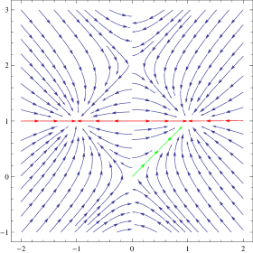
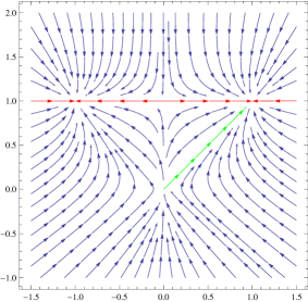
Figure 1: The pattern of flows for the two examples discussed in the text: $G=SU(2)$, $H=O(2)$ (left) and $G=SU(2)\times SU(2)$, $H=SU(2)_{\rm diag}$ (right). $\lambda$ and $\tilde{\lambda}$ are plotted respectively along the vertical and horizontal axis. The Kondo flows of the $G$-symmetric defects ($\lambda=\tilde{\lambda}$), analyzed in [8], are shown in green. The flows along the $\widehat{H}$-invariant subspaces ($\lambda=1$) are drawn in red. They descend to the Fredenhagen-Schomerus flows in the $G/H$ coset models. The symmetry $\tilde{\lambda}\rightarrow-\tilde{\lambda}$ corresponds to automorphisms of the algebras $\mathfrak{g}$, as explained in the text. Both cases have fixed points at $(0,0),(0,1)$ and $(1,\pm 1)$. In the first example, the first two fixed points lie on the $\lambda$ axis, which is a line of marginal deformations.

The second example of section 2.4 has $G=SU(2)\times SU(2)^{\prime}$, $H=SU(2)_{\rm diag}$ and a defect associated to a representation $R=(j,0)$ of $G$. The general Hamitlonian (31) has again two free parameters. It reads

$${\cal H}_{\rm imp}^{(j,0)}(\lambda,\tilde{\lambda})=-\frac{1}{2k}\Bigl{[}\lambda\,\vec{t}\cdot(\vec{\cal J}_{-}+\vec{\cal J}_{-}^{\prime})+\tilde{\lambda}\,\vec{t}\cdot(\vec{\cal J}_{-}-\vec{\cal J}_{-}^{\prime})\Bigr{]}\ ,$$

where $\vec{t}$ is the triplet of $SU(2)$ generators in the representation of spin $j$. A straightforward calculation leads to the following $\beta$-function equations in this example:

$${d\lambda_{\pm}\over dt} \ =\ \frac{8}{k}\lambda_{\pm}(\lambda_{\pm}-\lambda_{\pm}^{2}-\lambda_{\mp}^{2})+O\left({1\over k^{2}}\right)\ ,$$ (81)

where $\lambda_{\pm}=(\lambda\pm\tilde{\lambda})/2$ are the couplings to the two $SU(2)$ factors of $G$. The RG flow (81) is exhibited in the right-hand-side of Figure 1. Local gauge invariance fixes $\lambda=\lambda_{+}+\lambda_{-}=1$, leaving $\tilde{\lambda}$ as the only running coupling. On the diagonal line, $\lambda=\tilde{\lambda}$, the full global $G$ symmetry is restored. Finally, on the $\lambda$ axis only the currents of $SU(2)_{\rm diag}$ enter in the defect Hamiltonian. The flow diagram (79) is realized on these three invariant lines. The flow (in red) along the line $\lambda=1$ is the only one that descends to the coset model. The symmetry under the exchange $\lambda_{+}\leftrightarrow\lambda_{-}$ corresponds here to the outer automorphism exchanging the two factors of $G$.

5 Exact quantization and boundary flows

The non-perturbative quantization of the holomorphic defects for generic $M^{a}$ is at present an open problem. On the other hand, the special fixed-point operators which correspond to the classical monodromies (see section 3.3) can be quantized along the lines of [20] exactly. We will now explain how this works and then use the exact spectrum of the quantum monodromy traces to derive the generalized Affleck-Ludwig rule (10).

5.1 Exact quantization of the fixed-point defects

Throughout this section, we choose $R$ to be an irreducible representation of $G$ of highest weight $\mu$, and write ${O}_{\mu}^{\mathfrak{g}}$ and ${O}_{\mu}^{\mathfrak{h}}$ for the two fixed-point loop operators denoted ${O}_{R}^{\mathfrak{g}}$ and ${O}_{R}^{\mathfrak{h}}$ in the previous section. Closely related loop operators were constructed in ref. [20] in the context of ungauged WZW models. We will apply here the same quantization technique to construct the relevant operators in the ungauged WZW model and then check that they have well-defined actions on the state space of the gauged model (i.e. are gauge invariant).

Let us consider first the stable, maximally-symmetric fixed point at $M^{a}=T^{a}$. The central idea in [20] was to use two properties of the classical loop observable: it involves only the holomorphic current and it has vanishing Poisson bracket with it. Demanding these properties to be preserved by quantization, we ask that ${O}_{\mu}^{\mathfrak{g}}$ should be expressed as a series in the generators of $\hat{\mathfrak{g}}_{k}$ and that it commutes with all these generators. More precisely, ${O}_{\mu}^{\mathfrak{g}}$ should be a central element in an appropriate completion $\bar{U}(\hat{\mathfrak{g}}_{k})$ of the enveloping algebra $U(\hat{\mathfrak{g}}_{k})$. Building up on [58], a recursive algorithm was presented in [20] to compute the series expressing $O^{\mathfrak{g}}_{\mu}$ in terms of the currents $J^{G}$. As it is central, $O^{\mathfrak{g}}_{\mu}$ acts by scalar multiplication on each irreducible highest-weight module of $\hat{\mathfrak{g}}_{k}$. The quantization procedure also provides its eigenvalue:

$$O^{\mathfrak{g}}_{\mu}=\chi^{\mathfrak{g}}_{\mu}\left(-\frac{2\pi i}{k+\check{h}_{\mathfrak{g}}}(\nu+\rho_{\mathfrak{g}})\right)\mathbbm{1}\qquad\mbox{on }L^{\mathfrak{g}}_{(\nu,k)}\ .$$ (82)

Here $\chi^{\mathfrak{g}}_{\mu}$ is the character of $R$ seen as a function on the weight space of $\mathfrak{g}$, while $\check{h}_{\mathfrak{g}}$ and $\rho_{\mathfrak{g}}$ are the dual Coxeter number and the Weyl vector of $\mathfrak{g}$. In particular, if $\nu$ and $\mu$ are integrable weights of $\hat{\mathfrak{g}}_{k}$, then this expression simplifies to

$$O^{\mathfrak{g}}_{\mu}=\frac{S^{\mathfrak{g}}_{\mu\nu}}{S^{\mathfrak{g}}_{0\nu}}\mathbbm{1}\qquad\mbox{on }L^{\mathfrak{g}}_{(\nu,k)}\ ,$$ (83)

where $S^{\mathfrak{g}}_{\mu\nu}$ is the modular $S$-matrix element of $\hat{\mathfrak{g}}_{k}$. As noted in the introduction, and further discussed in subsection 3.3, $O^{\mathfrak{g}}_{\mu}$ is the quantum analog of the trace of the classical monodromy matrix (for early semi-classical studies, see [40, 41]).

A comment is in order here concerning the two fixed points, at $\tilde{\lambda}=\pm 1$, in the $SU(2)/O(2)$ example of section 4.4. Recall that the map $\tilde{\lambda}\rightarrow-\tilde{\lambda}$ can be implemented by conjugating the $SU(2)$ currents with the operator $\exp\left(\frac{\pi i}{\sqrt{2}}J^{3}_{0}\right)$. Since this commutes with $O^{\mathfrak{g}}_{\mu}$, we conclude that the loop operators at these two fixed points coincide.

Let us come now to the unstable fixed point at $(\Theta^{j},\tilde{\Theta}^{s})=(T^{j},0)$. Again, the corresponding classical loop observable is characterized by two facts: it is built out of the restriction of the WZW current to the subgroup $H$ and its Poisson bracket with the restricted current vanishes. We deduce that $O^{\mathfrak{h}}_{\mu}$ has to be an element of the center of the completed enveloping algebra $\bar{U}(\hat{\mathfrak{h}}_{kx})$ and it can be constructed along the same lines. Such operators were considered in [20] as loop operators breaking the chiral symmetry of the WZW model from $\hat{\mathfrak{g}}$ to $\hat{\mathfrak{h}}\times\hat{\mathfrak{g}}/\hat{\mathfrak{h}}$, where the second factor denotes the coset vertex algebra. The action of the quantum operator, $O^{\mathfrak{h}}_{\mu}$, on a highest weight $\hat{\mathfrak{h}}$-module $L^{\mathfrak{h}}_{(\beta,\kappa)}$ reads

$$O^{\mathfrak{h}}_{\mu}=\sum_{\alpha}b_{\mu\alpha}\,O^{\mathfrak{h}}_{\alpha}=\sum_{\alpha}b_{\mu\alpha}\,\chi^{\mathfrak{h}}_{\alpha}\left(-\frac{2\pi i}{\kappa+\check{h}_{\mathfrak{h}}}(\gamma+\rho_{\mathfrak{h}})\right)\mathbbm{1}\qquad\mbox{on }L^{\mathfrak{h}}_{(\gamma,\kappa)}\ ,$$ (84)

where $\kappa$ is the level and $\gamma$ is an integrable highest weight of the Kac-Moody algebra $\hat{\mathfrak{h}}_{\kappa}$. Furthermore, $b_{\mu\alpha}$ are the branching coefficients in the decomposition of $R$ in irreducible $\mathfrak{h}$-representations of highest weight $\alpha$. Note that here and in what follows we use Greek letters from the middle of the alphabet to denote highest weights, and corresponding representations of $\mathfrak{g}$, while letters from the beginning of the alphabet stand for highest weights and representations of the subalgebra $\mathfrak{h}$.

Let us now check the gauge invariance of the operators constructed. The coset modules, which form the building blocks of the state space of the coset model, are constructed by taking the quotient by the action of the Kac-Moody subalgebra $\hat{\mathfrak{h}}\subseteq\hat{\mathfrak{g}}$. Any operator commuting with the action of $\hat{\mathfrak{h}}$ has a well-defined action on the coset modules, and therefore on the state space of the coset model. But $O^{\mathfrak{g}}_{R}$ and $O^{\mathfrak{h}}_{R}$ commute with $\hat{\mathfrak{h}}\subseteq\hat{\mathfrak{g}}$ by construction. As a matter of fact, $O^{\mathfrak{g}}_{R}$ commutes with $\hat{\mathfrak{g}}$ and $O^{\mathfrak{h}}_{R}$, being a central element in $\hat{U}(\hat{\mathfrak{h}}_{kx})\subseteq\hat{U}(\hat{\mathfrak{g}}_{k})$, commutes with the action of $\hat{\mathfrak{h}}$. Using the decomposition (44) of the integrable modules of $\hat{\mathfrak{g}}_{k}$ in terms of modules of $\hat{\mathfrak{h}}_{xk}$ and modules of the coset vertex algebra, we deduce that the actions of the two fixed point operators are given by

$$O^{\mathfrak{g}}_{\mu}=\frac{S^{\mathfrak{g}}_{\mu\nu}}{S^{\mathfrak{g}}_{0\nu}}\mathbbm{1}\ ,\qquad\mbox{and}\ \ \ O^{\mathfrak{h}}_{\mu}=\sum_{\alpha}b_{\mu\alpha}\,\frac{S^{\mathfrak{h}}_{\alpha\gamma}}{S^{\mathfrak{h}}_{0\gamma}}\mathbbm{1}\qquad\mbox{on }\ \ L^{\mathfrak{g}/\mathfrak{h}}_{[\nu,\gamma]}\ ,$$ (85)

where $S^{\mathfrak{g}}$ and $S^{\mathfrak{h}}$ are the modular $S$-matrices for $\mathfrak{g}_{k}$ and $\mathfrak{h}_{xk}$, and $b_{\mu\alpha}$ the branching coefficients. Remark that they both act by scalar multiplication on the coset modules, and therefore commute with the action of the coset vertex algebra.

In appendix A we will show how to rederive the above results in the BRST quantization of the gauged WZW model.

5.2 The generalized Affleck-Ludwig rule

We have argued in this paper that there exist RG flows of holomorphic defects in the GKO model based on the coset $G/H$, which send

$$O^{\mathfrak{h}}_{\mu}\mapsto O^{\mathfrak{g}}_{\mu}\ ,$$ (86)

for any $G$-representation of highest weight $\mu$. These are the flows marked in red in the examples of figure 1. We have computed explicitly these flows at the leading order in $1/k$, and the loop operators at the two fixed points exactly. We have also explained in section 4 how the renormalized operator along the flow can be made to commute with translations on the cylinder. Following the ideas of [7, 8], we can thus push the defect to a conformal boundary and induce automatically a boundary RG flow. We will now explain how the flow (86) can be used to derive the generalized Affleck-Ludwig rule [43, 44, 45], i.e. expression (10) of the introduction.

We start by reviewing the construction of boundary states in coset models (see [45] for more details). Recall that the primary fields are labeled by pairs $(\mu,\alpha)$ of integrable weights for $\hat{\mathfrak{g}}_{k}$ and $\hat{\mathfrak{h}}_{xk}$. Not all of these pairs are admissible, and some pairs must be identified (see for instance [49], chapter 18). Let us write $[\mu,\alpha]$ for the equivalence classes of the admissible pairs, and denote by $\mathcal{P}$ the set of these equivalence classes. The modular S-matrix of the coset theory can be expressed in term of the modular S-matrices of $\hat{\mathfrak{g}}_{k}$ and $\hat{\mathfrak{h}}_{xk}$ as follows :

$$S^{\mathfrak{g}/\mathfrak{h}}_{[\mu,\alpha],[\nu,\beta]}=nS^{\mathfrak{g}}_{\mu\nu}(S^{\mathfrak{h}})^{-1}_{\alpha\beta}\ ,$$ (87)

where we chose particular representatives $(\mu,\alpha)$ and $(\nu,\beta)$ in the equivalence classes $[\mu,\alpha]$ and $[\nu,\beta]$, and $n$ denotes the number of pairs in each equivalence class. The right-hand side of (87) is, of course, independent of this choice.

We can construct conformal boundary states for this theory, starting with any representation of the fusion algebra by matrices with non-negative integer entries. More specifically, we consider a set of matrices $N_{[\mu,\alpha]}$, indexed by the primary fields of our coset model, with non-negative integer matrix elements $(N_{[\mu,\alpha]})_{I}^{\ J}$. These must form a representation of the fusion algebra:

$$N_{[\mu,\alpha]}\ N_{[\nu,\beta]}=\sum_{[\rho,\gamma]}\mathcal{N}_{[\mu,\alpha],[\nu,\beta]}^{\qquad[\rho,\gamma]}\ N_{[\rho,\gamma]}\ ,$$ (88)

where $\mathcal{N_{\rm XY}^{\ \ \rm Z}}$ are the fusion coefficients. They must furthermore obey the conditions

$$N_{[0,0]}=\mathbbm{1}\qquad\mbox{and }\ \ \ N_{[\mu,\alpha]}=(N_{[\mu^{\ast},\alpha^{\ast}]})^{T}\ ,$$ (89)

where $\mu^{\ast}$ is the weight conjugate to $\mu$. Now since the fusion rules form a commutative algebra, all of its irreducible representations are one-dimensional. The latter are labeled by the coset fields $[\nu,\beta]$ and given explicitly by

$$[\mu,\alpha]\mapsto\frac{S^{\mathfrak{g}/\mathfrak{h}}_{[\mu,\alpha],[\nu,\beta]}}{S^{\mathfrak{g}/\mathfrak{h}}_{[0,0],[\nu,\beta]}}\ .$$ (90)

The representation provided by $N$ decomposes into these irreducible representations as follows:

$$\sum_{J}(N_{[\mu,\alpha]})_{I}^{\ J}\ \psi_{J}^{[\nu,\beta],i}=\frac{S^{\mathfrak{g}/\mathfrak{h}}_{[\mu,\alpha],[\nu,\beta]}}{S^{\mathfrak{g}/\mathfrak{h}}_{[0,0],[\nu,\beta]}}\ \psi_{I}^{[\nu,\beta],i}\ ,$$ (91)

where $\psi^{[\nu,\beta],i}$ are the common eigenvectors of the matrices $N$. We included, for completeness, $i$ as a possible multiplicity index, and we denote this multiplicity by $n_{[\nu,\beta]}$. Attention: the indices in this subsection should not be confused with those in the rest of the paper.

Consider next the torus partition function of the coset model

$$Z(q,\bar{q})=Z_{[\mu,\alpha],[\nu,\beta]}\,\chi^{\mathfrak{g}/\mathfrak{h}}_{[\mu,\alpha]}(q)\,\chi^{\mathfrak{g}/\mathfrak{h}}_{[\nu,\beta]}(\bar{q})\ ,$$

where $\chi^{\mathfrak{g}/\mathfrak{h}}_{[\mu,\alpha]}(q)$ is the character of the coset module $L^{\mathfrak{g}/\mathfrak{h}}_{[\mu,\alpha]}$. Suppose moreover that there exists an automorphism $\Omega$ of the coset vertex algebra, such that $Z_{[\nu,\beta],\Omega[\nu,\beta]}=n_{[\nu,\beta]}$. We can then build an elementary boundary state for each value of the matrix index $I$ :

$$B_{I}\ \equiv\ \sum_{[\nu,\beta]\in\mathcal{P}}\ \frac{\psi^{[\nu,\beta],i}_{I}}{\sqrt{S^{\mathfrak{g}/\mathfrak{h}}_{[0,0],[\nu,\beta]}}}|\,[\nu,\beta],i\rangle\!\rangle\ ,$$ (92)

where $|\,[\nu,\beta],i\rangle\!\rangle$ are the Ishibashi states corresponding to the $n_{[\nu,\beta]}$ orthogonal coset modules, isomorphic to $L^{\mathfrak{g}/\mathfrak{h}}_{[\nu,\beta]}\otimes L^{\mathfrak{g}/\mathfrak{h}}_{\Omega[\nu,\beta]}$, in the closed-string spectrum.

We are at long last ready to compute the RG flows induced on conformal boundaries by our holomorphic-defect flow (86). Acting with the UV and IR fixed-point operators on the conformal boundary state $B_{I}$, and inserting the exact formulae (85), leads to:

$$\sum_{\alpha}b_{\mu\alpha}\sum_{[\nu,\gamma]\in\mathcal{P}}\frac{S^{\mathfrak{h}}_{\alpha\gamma}}{S^{\mathfrak{h}}_{0\gamma}}\frac{\psi^{[\nu,\gamma],i}_{I}}{\sqrt{S^{\mathfrak{g}/\mathfrak{h}}_{[0,0],[\nu,\gamma]}}}|\,[\nu,\gamma],i\rangle\!\rangle\mapsto\sum_{[\nu,\gamma]\in\mathcal{P}}\frac{S_{\mu\nu}}{S_{0\nu}}\frac{\psi^{[\nu,\gamma],i}_{I}}{\sqrt{S^{\mathfrak{g}/\mathfrak{h}}_{[0,0],[\nu,\gamma]}}}|\,[\nu,\gamma],i\rangle\!\rangle\ .$$ (93)

Using the identities (which follow from (87))

$$\left(\frac{S^{\mathfrak{h}}_{\alpha\gamma}}{S^{\mathfrak{h}}_{0\gamma}}\right)^{-1}\ =\ \frac{S^{\mathfrak{g}/\mathfrak{h}}_{[0,\alpha],[\nu,\gamma]}}{S^{\mathfrak{g}/\mathfrak{h}}_{[0,0],[\nu,\gamma]}}\qquad\mbox{and}\qquad\frac{S^{\mathfrak{g}}_{\mu\nu}}{S^{\mathfrak{g}}_{0\nu}}=\frac{S^{\mathfrak{g}/\mathfrak{h}}_{[\mu,0],[\nu,\gamma]}}{S^{\mathfrak{g}/\mathfrak{h}}_{[0,0],[\nu,\gamma]}}\ ,$$ (94)

as well as the definition (91) of the coefficients $\psi$, we finally find the boundary flows:

$$\sum_{\alpha}b_{\mu\alpha}\sum_{J}(N_{[0,\alpha]})_{I}^{\ J}B_{J}\ \ \mapsto\ \ \sum_{J}(N_{[\mu,0]})_{I}^{\ J}B_{J}\ .$$ (95)

This is precisely the generalization of the Affleck-Ludwig rule to coset models described in refs. [43, 44, 45]. The RG flows (10) of the introduction are a special instance of the above rule, where $N_{[\mu,0]}$ are replaced by the fusion matrices ${\cal N}_{[\mu,0]}$ (and the matrix indices $I,J\cdots$ run over $\mathcal{P}$). The fusion matrices form themselves a representation of the fusion algebra, and the boundary states constructed out of them are the maximally symmetric boundary states first constructed by Cardy [39]. Note, as a consistency check, that the coefficients of the boundary states on both sides of (95) are non-negative integers. For a detailed account of the boundary RG flows falling in the scope of the generalized Affleck-Ludwig rule in the critical Ising model, the tricritical Ising model and the three states Potts model, see the appendix B of [45]. Our derivation of this rule from flows of holomorphic bulk defects shows its universality, in particular the fact that the beta functions are independent of the boundary condition.

Let us note in closing that bulk defects of a conformal field theory, A, can be viewed via the folding trick [5, 59] as boundaries of the theory A$\otimes{P}({\rm A})$, where ${P}$ is the parity transformation. Equations (9) on the other hand suggest that, in certain situations, holomorphic defects can be in one-to-one correspondence with boundaries of the (single-copy) theory A. “Under what conditions does this happen?” is a question that deserves further investigation.

Aknowledgements We thank Anton Alekseev, Ilka Brunner, Denis Bernard, Ingo Runkel, Samson Shatashvili and Kostya Zarembo for discussions. This work has been supported by the European Networks ’Superstring Theory’ (MRTN-CT-2004-512194) and ‘Forces Universe’ (MRTN-CT-2004-005104) and by the Agence Nationale pour la Recherche (contract 05-BLAN-0079-01). S.M. is supported in part by the fellowship PBGE2–121187 of the Swiss National Science Foundation.

Appendix A Quantum monodromies in the BRST scheme

We have seen in this paper that the endpoints of the Fredenhagen-Schomerus flows were defects with classical couplings $(\Theta^{j},\tilde{\Theta}^{s})=(T^{j},0)$ and $(T^{j},T^{s})$. In section 5.1 we have constructed, in the GKO quantization scheme, the corresponding quantum-monodromy operators $O^{\mathfrak{h}}_{\mu}$ and $O^{\mathfrak{g}}_{\mu}$. We will here show that the same result can be obtained in the BRST quantization. The starting point in the BRST scheme is the expression (48) for the impurity Hamiltonian, with the choice $\tilde{\Theta}^{j}=T^{j}$ for the unphysical couplings. With this choice, at the two endpoints of the flow the defect couples only to the currents, respectively, of $H$ and $G$. The two fixed-point operators are thus central elements in the enveloping algebras of the two independent Kac-Moody algebras: $\hat{\mathfrak{g}}$ at level $k$ and $\hat{\mathfrak{h}}$ at level $-xk-2\check{h}_{\mathfrak{h}}$. We will show that these fixed-point operators have the same action as their counterparts in the GKO quantization of the model.

Let us first review briefly how one derives in the BRST scheme the GKO space of states described in section 3.2. For more details we refer the reader to [51, 53]. Recall that we have an embedding $\hat{\mathfrak{h}}\subseteq\hat{\mathfrak{g}}$ of Kac-Moody algebras for each embedding of finite semisimple Lie algebras $\mathfrak{h}\subseteq\mathfrak{g}$. Accordingly, a highest weight integrable module $L^{\mathfrak{g}}_{(\nu,k)}$ for $\hat{\mathfrak{g}}$ at level $k$ decomposes into $\hat{\mathfrak{h}}$-modules at level $xk$ according to eq. (44),

$$L^{\mathfrak{g}}_{(\nu,k)}=\bigoplus_{\gamma}L^{\mathfrak{h}}_{(\gamma,xk)}\otimes L^{\mathfrak{g}/\mathfrak{h}}_{[\nu,\gamma]}\ .$$

The coset modules $L^{\mathfrak{g}/\mathfrak{h}}_{[\nu,\gamma]}$ carry an action of the coset vertex algebra, which is composed of all the normal-ordered products of generators of $\hat{\mathfrak{g}}$ that commute with every element in $\hat{\mathfrak{h}}$. These modules are the building blocks of the state space of the GKO coset models.

By contrast in the BRST scheme the classical currents $\mathcal{J}^{G}$ and $\mathcal{J}^{H}$ are quantized separately into generators $J^{G}$ and $J^{H}$, and the gauged WZW model starts out as a direct product of three non-interacting theories:

• a WZW theory based on $G$ at level $k$, with current $J^{G}$;

• a WZW theory based on $H$ at level $-xk-2\check{h}_{\mathfrak{h}}$, with current $J^{H}$, where $x$ is the embedding index of $\mathfrak{h}$ in $\mathfrak{g}$, and $\check{h}_{\mathfrak{h}}$ is the dual Coxeter number of $\mathfrak{h}$; and

• a system of ghosts in the adjoint representation of $\mathfrak{h}$.

As a result, the extended space before the BRST projection to physical states, is made out of tensor products of three highest-weight modules:

$$L^{\mathfrak{g}}_{(\nu,k)}\otimes L^{\mathfrak{h}}_{(-\gamma-2\rho_{\mathfrak{h}},-xk-2\check{h}_{\mathfrak{h}})}\otimes L^{\mbox{\tiny ghosts}}\ .$$ (96)

Here $\nu$ is an integrable weight of $\hat{\mathfrak{g}}_{k}$, $\gamma$ an integrable weight of $\hat{\mathfrak{h}}_{xk}$, $\rho_{\mathfrak{h}}$ is the Weyl vector of ${\mathfrak{h}}$ (the half sum of its positive roots), and $L^{\mbox{\tiny ghosts}}$ is a module for the ghost algebra which plays a spectator role in our discussion. It is understood that ${J}^{G}$ acts on the first factor and ${J}^{H}$ on the second one. A basis of representatives of the relative BRST cohomology of this module is provided by states such that [53]:

• their component in the first factor lies in a given summand $L^{\mathfrak{h}}_{(\gamma,xk)}\otimes L^{\mathfrak{g}/\mathfrak{h}}_{[\nu,\gamma]}$ of (44), and is of the form $|\,0,\gamma,xk\rangle\otimes|\,\phi\rangle$, where the first state is the highest weight vector of $L^{\mathfrak{h}}_{(\gamma,xk)}$ while the second is an arbitrary state of $L^{\mathfrak{g}/\mathfrak{h}}_{[\nu,\gamma]}$ ;

• their component in the second factor is the highest weight vector $|\,0,-\gamma-2\rho_{\mathfrak{h}},-xk-2\check{h}_{\mathfrak{h}}\rangle$;

• their ghost component is the ghost vacuum $|\,0,\mbox{ghosts}\rangle$.

It follows rather easily that the relative BRST cohomology of (96) is isomorphic to $L^{\mathfrak{g}/\mathfrak{h}}_{[\nu,\gamma]}$. As the latter is the building block of the GKO construction of the state space, the equivalence of the BRST and GKO approaches at the level of state space can be established.

Let us now go back to the fixed-point operators $O^{\mathfrak{g}}_{\mu}$ and $O^{\mathfrak{h}}_{\mu}$. To each state $|\,\phi\rangle\in L^{\mathfrak{g}/\mathfrak{h}}_{[\nu,\gamma]}$ in the GKO construction corresponds a representative

$$|\,\phi_{\rm BRST}\rangle=|\,0,\gamma,xk\rangle\otimes|\,\phi\rangle\otimes|\,0,-\gamma-2\rho_{\mathfrak{h}},-xk-2\check{h}_{\mathfrak{h}}\rangle\otimes|\,0,\mbox{ghosts}\rangle$$ (97)

in the relative BRST cohomology of the gauged WZW model. The IR operator $O^{\mathfrak{g}}_{\mu}$ acts on the first two factors of (97), i.e. on a state in the module $L^{\mathfrak{g}}_{(\nu,k)}$ of $\mathfrak{g}_{k}$. Its action is thus given by (82), i.e. it is the same as in the GKO quantization.

The story is more interesting for the UV operator $O^{\mathfrak{h}}_{\mu}$ which acts on the third factor in the decomposition (97). Our first task is to establish that the central elements constructed in [58, 20] have a well-defined action on the Kac-Moody modules for $\hat{\mathfrak{h}}$ at the subcritical level $-\check{h}_{\mathfrak{h}}-2k$. Let us recall how central operators in a completion of the universal enveloping algebra of $\hat{\mathfrak{h}}$ were constructed by a recursive procedure in these references. First consider the triangular decomposition of $\hat{\mathfrak{h}}$ : $\hat{\mathfrak{h}}=\hat{\mathfrak{h}}_{+}\oplus\hat{\mathfrak{h}}_{0}\oplus\hat{\mathfrak{h}}_{-}$, where $\hat{\mathfrak{h}}_{0}$ is the Cartan subalgebra. Define the following functions on the affine weight space $(\hat{\mathfrak{h}}_{0})^{\ast}$ :

$$T_{\omega}(\alpha)=2(\alpha+\hat{\rho}_{\mathfrak{h}}-\omega,\omega)\ ,$$

where the index $\omega$ is an element of the affine root lattice, and $\hat{\rho}_{\mathfrak{h}}$ is the affine Weyl vector of $\hat{\mathfrak{h}}$. (Recall that the affine Weyl vector has a horizontal part equal to the Weyl vector $\rho_{\mathfrak{h}}$ of the horizontal Lie algebra $\mathfrak{h}$ and a level equal to the dual Coxeter number $\check{h}_{\mathfrak{h}}$.) Consider also the subset $L\subset(\hat{\mathfrak{h}}_{0})^{\ast}$, defined by $\alpha\in L\Leftrightarrow T_{n\psi}(\alpha+\varphi)\neq 0$ for each positive affine root $\psi$, each positive integer $n$, and $\varphi$ in the affine root lattice. Given any function $f$ analytic on $L$, it is possible to construct a central operator which has a well defined action on every module with highest weight $\alpha\in L$. The central operator acts on the module with highest weight $\alpha$ by scalar multiplication by $f(\alpha)$. Note that these modules are exactly the irreducible Verma modules of the Kac-Moody algebra, and that $L$ contains neither the integrables weights nor the weights at negative level appearing in the state space of the gauged WZW model.

In order to obtain a central operator that is well-defined on integrable modules, additional conditions must be imposed on the function $f$ defining the operator. These conditions take the following form [58] :

$$T_{n\psi}(\alpha)=0\qquad\Rightarrow\qquad f(\alpha)=f(\alpha-n\psi)$$ (98)

for $\psi$ a real positive root. A slightly stronger but more conceptual condition is that $f$ should be invariant under the action of the Weyl group shifted by the Weyl vector $\rho_{\mathfrak{h}}$. One can easily check that the function (82) used to define Wilson operators satisfies this property. When the conditions (98) are satisfied, it is proved in [58] (Theorem 2) that the central operator has a well defined action on any highest weight module whose highest weight lies in $-\hat{\rho}_{\mathfrak{h}}+K$, where $K$ is the Tits cone of $\hat{\mathfrak{h}}$. The Tits cone is defined as the set of all the weights which have negative scalar product with a finite number of roots only. The set $-\hat{\rho}_{\mathfrak{h}}+K$ does contain all the integrable weights of $\hat{\mathfrak{h}}$, but not our subcritical level weights. Indeed, a weight with negative level never belongs to $K$, because its scalar product with roots of sufficiently high grade would always be negative. Therefore, weights with level below the critical level $-\check{h}_{\mathfrak{h}}$ cannot belong to $-\hat{\rho}_{\mathfrak{h}}+K$, and we cannot use Theorem 2 of [58] to conclude that our operators have a well-defined action on the $\hat{\mathfrak{h}}$-modules entering the BRST quantization of the gauged WZW model.

However, a careful analysis of the proof of this theorem shows that whenever the condition (98) is satisfied, the action of central operators can be extended across the planes $T_{n\psi}(\alpha)=0$ for any $\psi$ such that $(\psi,\psi)>0$. So it may be impossible to perform this extension only on weights satisfying $T_{n\Psi}(\alpha)=0$, where $\Psi$ is the imaginary simple root of the Kac-Moody algebra. The scalar product of $\Psi$ with an affine weight gives the level of this weight, so for a generic affine weight $\alpha$ of level $\kappa$, we have

$$T_{n\Psi}(\alpha)=2(\alpha+\hat{\rho}_{\mathfrak{h}}-n\Psi,n\Psi)=2n(\kappa+\check{h}_{\mathfrak{h}})\ .$$ (99)

The extension may therefore fail only for weights with critical level $\kappa=-\check{h}_{\mathfrak{h}}$. This is not the case in the problem at hand, since $k>0$ so that our weights are strictly subcritical. We conclude that the quantum-monodromy operators do have a well-defined action on each of the modules appearing in the state space of the gauged WZW model in the BRST quantization.

This rather lengthy argument shows that we can compute the action of $O^{\mathfrak{h}}_{\mu}$ on the third factor of (97) by using eq. (84) with the replacements: $\gamma\to-\gamma-2\rho_{\mathfrak{h}}$ and $\kappa\to-xk-2\check{h}_{\mathfrak{h}}$. From the trivial identity

$$-\frac{2\pi i}{xk+\check{h}_{\mathfrak{h}}}(\gamma+\rho_{\mathfrak{h}})\,=\,-\frac{2\pi i}{(-xk-2\check{h}_{\mathfrak{h}})+\check{h}_{\mathfrak{h}}}\left((-\gamma-2\rho_{\mathfrak{h}})+\rho_{\mathfrak{h}}\right)$$ (100)

we then conclude that the action of this fixed-point operator is the same in the GKO and BRST quantizations of the gauged WZW model.

References

- [1] V. V. Bazhanov, S. L. Lukyanov and A. B. Zamolodchikov, “Integrable structure of conformal field theory, quantum KdV theory and thermodynamic Bethe ansatz”, Commun. Math. Phys. 177 (1996) 381–398, hep-th/9412229.
- [2] V. V. Bazhanov, S. L. Lukyanov and A. B. Zamolodchikov, “Integrable structure of conformal field theory II. Q-operator and DDV equation”, Commun. Math. Phys. 190 (1997) 247–278, hep-th/9604044.
- [3] V. V. Bazhanov, S. L. Lukyanov and A. B. Zamolodchikov, “Integrable structure of conformal field theory. III: The Yang-Baxter relation”, Commun. Math. Phys. 200 (1999) 297–324, hep-th/9805008.
- [4] C. L. Kane and M. P. A. Fisher, “Transmission through barriers and resonant tunneling in an interacting one-dimensional electron gas”, Phys. Rev. B46 (1992) 15233.
- [5] M. Oshikawa and I. Affleck, “Boundary conformal field theory approach to the critical two-dimensional Ising model with a defect line”, Nucl. Phys. B495 (1997) 533–582, cond-mat/9612187.
- [6] For a recent reference see, for example, P. Fendley, M. P. A. Fisher and C. Nayak, “Boundary Conformal Field Theory and Tunneling of Edge Quasiparticles in non-Abelian Topological States”, Annals Phys. 324 (2009) 1547–1572, cond-mat/0902.0998.
- [7] K. Graham and G. M. T. Watts, “Defect lines and boundary flows”, JHEP 0404 (2004) 019 hep-th/0306167.
- [8] C. Bachas and M. Gaberdiel, “Loop operators and the Kondo problem”, JHEP 0411 (2004) 065, hep-th/0411067.
- [9] S. Fredenhagen, M. R. Gaberdiel and C. Schmidt-Colinet, “Bulk flows in Virasoro minimal models with boundaries”, arXiv:0907.2560 [hep-th].
- [10] S. Monnier, “New WZW D-branes from the algebra of Wilson loop operators”, JHEP 0910 (2009) 016, arXiv:0907.2921 [hep-th].
- [11] I. Brunner, D. Roggenkamp and S. Rossi, “Defect Perturbations in Landau-Ginzburg Models”, arXiv:0909.0696 [hep-th].
- [12] M. Kormos, I. Runkel and G. M. T. Watts, “Defect flows in minimal models”, arXiv:0907.1497 [hep-th].
- [13] C. Bachas, “On the Symmetries of Classical String Theory”, arXiv:0808.2777 [hep-th].
- [14] J. Fröhlich, J. Fuchs, I. Runkel and C. Schweigert, “Kramers-Wannier duality from conformal defects”, Phys. Rev. Lett. 93 (2004) 070601, cond-mat/0404051.
- [15] J. Fröhlich, J. Fuchs, I. Runkel and C. Schweigert, “Duality and defects in rational conformal field theory”, Nucl. Phys. B763 (2007) 354–430, hep-th/0607247.
- [16] I. Brunner, H. Jockers and D. Roggenkamp, “Defects and D-Brane Monodromies”, arXiv:0806.4734 [hep-th].
- [17] V. B. Petkova and J. B. Zuber, “Generalised twisted partition functions”, Phys. Lett. B504 (2001) 157–164, hep-th/0011021.
- [18] T. Quella and V. Schomerus, “Symmetry breaking boundary states and defect lines”, JHEP 0206 (2002) 028, hep-th/0203161.
- [19] T. Quella, I. Runkel and G. M. T. Watts, “Reflection and Transmission for Conformal Defects”, JHEP 0704 (2007) 095, hep-th/0611296.
- [20] A. Alekseev and S. Monnier, “Quantization of Wilson loops in Wess-Zumino-Witten models”, JHEP 08 (2007) 039, hep-th/0702174.
- [21] A. Mikhailov and S. Schafer-Nameki, “Perturbative study of the transfer matrix on the string worldsheet in AdS(5)xS(5)”, arXiv:0706.1525[hep-th].
- [22] I. Brunner and D. Roggenkamp, “B-type defects in Landau-Ginzburg models”, JHEP 0708 (2007) 093, arXiv:0707.0922[hep-th].
- [23] I. Runkel, “Perturbed Defects and T-Systems in Conformal Field Theory”, J. Phys. A41 (2008) 105401, arXiv:0711.0102 [hep-th].
- [24] C. Bachas and I. Brunner, “Fusion of conformal interfaces”, JHEP 0802 (2008) 085, arXiv:0712.0076[hep-th].
- [25] I. Brunner and D. Roggenkamp, “Defects and Bulk Perturbations of Boundary Landau-Ginzburg Orbifolds”, JHEP 0804 (2008) 001, arXiv:0712.0188[hep-th].
- [26] D. Gang and S. Yamaguchi, “Superconformal defects in the tricritical Ising model”, JHEP 0812 (2008) 076, arXiv:0809.0175 [hep-th].
- [27] G. Sarkissian and C. Schweigert, “Some remarks on defects and T-duality”, Nucl. Phys. B819 (2009) 478–490, arXiv:0810.3159 [hep-th].
- [28] G. Sarkissian, “Defects and Permutation branes in the Liouville field theory”, arXiv:0903.4422 [hep-th].
- [29] P. Goddard, A. Kent, and D. I. Olive, “Virasoro algebras and coset space models”, Phys. Lett. B152 (1985) 88–92.
- [30] P. Goddard, A. Kent, and D. I. Olive, “Unitary Representations of the Virasoro and Supervirasoro Algebras”, Commun. Math. Phys. 103 (1986) 105–119.
- [31] O. Babelon, D. Bernard, and M. Talon, Introduction to Classical Integrable Systems. Cambridge University Press, February, 2007.
- [32] P. Bowcock, “Canonical Quantization of the Gauged Wess-Zumino Model”, Nucl. Phys. B316 (1989) 80–100.
- [33] K. Gawedzki and A. Kupiainen, “G/H conformal field theory from gauged WZW model”, Phys. Lett. B215 (1988) 119–123.
- [34] K. Gawedzki and A. Kupiainen, “Coset Construction from Functional Integrals”, Nucl. Phys. B320 (1989) 625.
- [35] D. Karabali, Q.-H. Park, H. J. Schnitzer, and Z. Yang, “A GKO construction based on a path integral formulation of gauged Wess-Zumino-Witten actions”, Phys. Lett. B216 (1989) 307–312.
- [36] A. Y. Alekseev, A. Recknagel, and V. Schomerus, “Brane dynamics in background fluxes and non-commutative geometry”, JHEP 05 (2000) 010, hep-th/0003187.
- [37] S. Monnier, “D-branes in Lie groups of rank 1”, JHEP 08 (2005) 062, hep-th/0507159.
- [38] I. Affleck and A. W. W. Ludwig, “The Kondo effect, conformal field theory and fusion rules”, Nucl. Phys. B352 (1991) 849–862.
- [39] J. L. Cardy, “Boundary Conditions, Fusion Rules And The Verlinde Formula”, Nucl. Phys. B324 (1989) 581–596.
- [40] D. Gepner and E. Witten, “String Theory on Group Manifolds”, Nucl. Phys. B 278 (1986) 493–549.
- [41] A. Alekseev and S. L. Shatashvili, “Quantum Groups and WZW Models”, Commun. Math. Phys. 133 (1990) 353–368.
- [42] A. Y. Alekseev, S. Fredenhagen, T. Quella, and V. Schomerus, “Non-commutative gauge theory of twisted D-branes”, Nucl. Phys. B646 (2002) 127–157, hep-th/0205123.
- [43] S. Fredenhagen and V. Schomerus, “D-branes in coset models”, JHEP 02 (2002) 005, hep-th/0111189.
- [44] S. Fredenhagen and V. Schomerus, “On boundary RG-flows in coset conformal field theories”, Phys. Rev. D67 (2003) 085001, hep-th/0205011.
- [45] S. Fredenhagen, “Organizing boundary RG flows”, Nucl. Phys. B660 (2003) 436–472, hep-th/0301229.
- [46] J. M. Maldacena, “Wilson loops in large N field theories”, Phys. Rev. Lett. 80 (1998) 4859–4862, hep-th/9803002.
- [47] S. J. Rey and J. T. Yee, “Macroscopic strings as heavy quarks in large N gauge theory and anti-de Sitter supergravity”, Eur. Phys. J. C 22, 379 (2001) hep-th/9803001..
- [48] E. Witten, “Nonabelian bosonization in two dimensions”, Commun. Math. Phys. 92 (1984) 455–472.
- [49] P. Di Francesco, P. Mathieu, and D. Sénéchal, Conformal Field Theory. Springer, 1997.
- [50] R. Dovgard and D. Gepner, “On conformal field theories with low number of primary fields”, arXiv:0811.1904[hep-th].
- [51] D. Karabali and H. J. Schnitzer, “BRST quantization of the gauged WZW action and coset conformal field theories”, Nuclear Physics B 329 (Jan., 1990) 649–666.
- [52] E. Witten, “On Holomorphic factorization of WZW and coset models”, Commun. Math. Phys. 144 (1992) 189–212.
- [53] S. Hwang and H. Rhedin, “The BRST Formulation of G/H WZNW models”, Nucl. Phys. B406 (1993) 165–186, hep-th/9305174.
- [54] K. Hori, “Global aspects of gauged wess-zumino-witten models”, Commun. Math. Phys. 182 (1996) 1–32, hep-th/9411134.
- [55] K. Gawedzki, “Boundary wzw, g/h, g/g and cs theories”, Annales Henri Poincare 3 (2002) 847–881, hep-th/0108044.
- [56] C. Bachas, J. Hoppe and B. Pioline, “Nahm equations, N = 1* domain walls, and D-strings in AdS(5) x S(5)”, JHEP 0107 (2001) 041, hep-th/0007067.
- [57] P. B. Kronheimer, “Instantons and the geometry of the nilpotent variety”, J. Diff. Geom. 32 (1990) 473.
- [58] V. G. Kac, “Laplace operators of infinite-dimensional Lie algebras and theta functions”, Proc. Nat. Acad. Sci. U.S.A. 81 (1984), no. 2, Phys. Sci., 645–647.
- [59] C. Bachas, J. de Boer, R. Dijkgraaf and H. Ooguri, “Permeable conformal walls and holography”, JHEP 0206 (2002) 027, hep-th/0111210.