Parallel Proximal Algorithm for Image Restoration Using Hybrid Regularization – Extended Version

Abstract

Regularization approaches have demonstrated their effectiveness for solving ill-posed problems. However, in the context of variational restoration methods, a challenging question remains, namely how to find a good regularizer. While total variation introduces staircase effects, wavelet domain regularization brings other artefacts, e.g. ringing. However, a trade-off can be made by introducing a hybrid regularization including several terms non necessarily acting in the same domain (e.g. spatial and wavelet transform domains). While this approach was shown to provide good results for solving deconvolution problems in the presence of additive Gaussian noise, an important issue is to efficiently deal with this hybrid regularization for more general noise models. To solve this problem, we adopt a convex optimization framework where the criterion to be minimized is split in the sum of more than two terms. For spatial domain regularization, isotropic or anisotropic total variation definitions using various gradient filters are considered. An accelerated version of the Parallel Proximal Algorithm is proposed to perform the minimization. Some difficulties in the computation of the proximity operators involved in this algorithm are also addressed in this paper. Numerical experiments performed in the context of Poisson data recovery, show the good behaviour of the algorithm as well as promising results concerning the use of hybrid regularization techniques.

1 Introduction

During the last decades, convex optimization methods have been shown to be very effective for solving inverse problems. On the one hand, algorithms such as Projection Onto Convex Sets (POCS) [2, 3, 4, 5, 6] have become popular for finding a solution in the intersection of convex sets. POCS was used in data recovery problems [7] in order to incorporate prior information on the target image (e.g. smoothness constraints). Some variants of POCS such as ART (Algebraic Reconstruction Technique) [8] or PPM (Parallel Projection Method) [9, 10] were also proposed to achieve iteration parallelization. Additional variants of POCS can be found in [11]. Other parallel approaches such as block-iterative surrogate constraint splitting methods were considered to solve a quadratic minimization problem under convex constraints [12] which may include a total variation constraint (see also [13]). However the method in [12] based on subgradient projections is not applicable to non-differentiable objective functions.

On the other hand, some denoising approaches were based on wavelet transforms [14], and more generally on frame representations [15, 16, 17, 18]. In [19, 20, 21, 22], algorithms which belong to the class of forward-backward algorithms were proposed in order to restore images degraded by a linear operator and a noise perturbation. Forward-backward iterations allow us to minimize a sum of two functions assumed to be in the class $\Gamma_{0}({\mathcal{H}})$ of lower semicontinuous convex functions defined on a Hilbert space ${\mathcal{H}}$, and taking their values in $]-\infty,+\infty]$, which are proper (i.e. not identically equal to $+\infty$). In addition, one of these functions must be Lipschitz differentiable on ${\mathcal{H}}$. In [23], this algorithm was investigated by making use of proximity operator tools [24] firstly proposed by Moreau in [25]. In [26], applications to frame representations were developed and a list of closed form expressions of several proximity operators was provided. Typically, forward-backward methods are appropriate when dealing with a smooth data fidelity term e.g. a quadratic function and a non-smooth penalty term such as an $\ell_{1}$-norm promoting sparsity in the considered frame [27, 28]. The computation of the proximity operator associated with the $\ell_{1}$-norm indeed reduces to a componentwise soft-thresholding [29, 30]. Another optimization method known as the Douglas-Rachford algorithm [31, 32, 33, 34] was then proposed for signal/image recovery problems [34] to relax the Lipschitz differentiablity condition required in forward-backward iterations. In turn, the latter algorithm requires the knowledge of the proximity operators of both functions. This algorithm was then extended to the minimization of a sum of a finite number of convex functions [35], the proximity operator of each function still being assumed to be known. One of the main advantages of this algorithm called Parallel ProXimal Algorithm (PPXA) is its parallel structure which makes it easily implementable on multicore architectures. PPXA is well suited to deconvolution problems in the presence of additive Gaussian noise, where the proximity operator associated with the fidelity term takes a closed form [35]. To minimize a sum of two functions one of which is quadratic, another interesting class of parallel convex optimization algorithms was proposed by Fornasier et al. in [36, 37]. However, in a more general context, particularly when the noise is not additive Gaussian and a wider class of degradation operators is considered, the proximity operator associated with data fidelity term does not have a closed form, which prevents the direct use of PPXA and the algorithms in [36] and [37]. Therefore, other solutions have to be looked for. For Poisson noise, a first solution is to resort to the Anscombe transform [38], while a second one consists of approximating the Poisson data fidelity term with a gradient Lipschitz function [39]. Both approaches require the use of a nested iterative algorithm [38, 39], combining forward-backward and Douglas-Rachford iterations. Nested algorithms may however appear limited for two main reasons: the parallelization of the related iterations is difficult, and the number of functions to be minimized is in practice limited to three. More recently, approaches related to augmented Lagrangian techniques [40, 41] have been considered in [42, 43, 44, 45]. These methods are well-adapted when the linear operator is a convolution and Fourier diagonalization techniques can thus be used, but for more general linear degradation operators, a large-size linear system of equations has to be solved numerically at each iteration of the algorithm.

The objective of this paper is to propose an adaptation of PPXA to minimize criteria used in a wide panel of restoration problems such as those involving a convolution or decimated convolution operator using a finite-support kernel and non-necessarily additive Gaussian noise. Decimated convolutions are important in practice since they are often encountered in super-resolution problems. To apply proximal methods, it seems that we should be able to compute the proximity operator associated with the fidelity term for a large class of noise distributions. When the proximity operator cannot be easily computed, we will show that a splitting approach may often be employed to circumvent this difficulty. This is the main contribution of this paper.

Moreover, based on similar splitting techniques and in the spirit of existing works on deconvolution in the presence of Gaussian noise [21, 35, 46, 47], a twofold regularization composed of a sparsity term and a total variation term is performed in order to benefit from each regularization. We will consider this type of hybrid regularization by investigating different discrete forms of the total variation.

The paper is organized as follows: first, in Section 2, we present the considered restoration problem and the general form of the associated criterion to be minimized. Then, in Section 3, the definition and some properties of proximity operators as well as explicit forms related to the data fidelity term in a restoration context and to a discretization of the total variation are provided. Section 4 introduces an accelerated version of PPXA which allows us to efficiently solve frame-based image recovery problems. Section 5.1 shows how the results obtained in the two previous sections can be used for solving restoration problems where a regularization is performed both in the spatial and in the wavelet domains. Finally, in Section 5.2, the effectiveness of the proposed approach is demonstrated by experiments for the restoration of images degraded by a blur (or a decimated blur) with finite-support kernel and by a Poisson noise. Some conclusions are drawn in Section 6.

2 Background

2.1 Image restoration

The degradation model considered throughout this paper is the following:

$$z=\mathcal{D_{\alpha}}(T\overline{y})$$ (1)

where $\overline{y}$ denotes the original image of global size $N$ degraded by a non-negative valued convolutive operator $T:\mathbb{R}^{N}\rightarrow\mathbb{R}^{M}$ and contaminated by a noise non necessarily additive, the effect of which is denoted by $\mathcal{D_{\alpha}}$. Here, $\alpha$ is a positive parameter which characterizes the noise intensity. The vector $z\in\mathbb{R}^{M}$ represents the observed data of size $M$. For example, $\mathcal{D_{\alpha}}$ may denote the addition of a zero-mean Laplacian noise with standard-deviation $\alpha$, or the corruption by an independent Poisson noise with scaling parameter $\alpha$. $T$ represents a convolution or a decimated convolution operator using a finite-support kernel.

Our objective is to recover the image $\overline{y}$ from the observation $z$ by using some prior information on its frame coefficients and its spatial properties.

2.2 Frame representation

In inverse problems, certain physical properties of the target solution $\overline{y}$ are most suitably expressed in terms of the coefficients $\overline{x}=(\overline{x}^{(k)})_{1\leq k\leq K}\in\mathbb{R}^{K}$ of its representation $\overline{y}=\sum_{k=1}^{K}\overline{x}^{(k)}e_{k}$ with respect to a family of vectors $(e_{k})_{1\leq k\leq K}$ in the Euclidean space $\mathbb{R}^{N}$. Recall that a family of vectors $(e_{k})_{1\leq k\leq K}$ in $\mathbb{R}^{N}$ constitutes a frame if there exist two constants $\underline{\nu}$ and $\overline{\nu}$ in $\,\left]0,+\infty\right[$ such that

$$(\forall y\in\mathbb{R}^{N})\qquad\underline{\nu}\|y\|^{2}\leq\sum_{k=1}^{K}|{e_{k}}^{\top}{y}|^{2}\leq\overline{\nu}\|y\|^{2}.\;$$ (2)

The associated frame operator is the injective linear operator $F\colon\mathbb{R}^{N}\to\mathbb{R}^{K}\colon y\mapsto({e_{k}}^{\top}{y})_{1\leq k\leq K}$, the adjoint of which is the surjective linear operator $F^{\top}\colon\mathbb{R}^{K}\to\mathbb{R}^{N}\colon(x^{(k)})_{1\leq k\leq K}\mapsto\sum_{k=1}^{K}x^{(k)}e_{k}$. When $\underline{\nu}=\overline{\nu}=\nu$ in (2), $(e_{k})_{1\leq k\leq K}$ is said to be a tight frame. In this case, we have

$$F^{\top}F=\nu\mathrm{Id},$$ (3)

where $\mathrm{Id}$ denotes the identity matrix. A simple example of a tight frame is the union of $\nu$ orthonormal bases, in which case $\underline{\nu}=\overline{\nu}=\nu$. For instance, a 2D real (resp. complex) dual-tree wavelet decomposition is the union of two (resp. four) orthonormal wavelet bases [18]. Curvelets [15] constitute another example of tight frame. Historically, Gabor frames [48] have played an important role in many inverse problems. Under some conditions, contourlets [49] also constitute tight frames. When $F^{-1}=F^{\top}$, an orthonormal basis is obtained. Further constructions as well as a detailed account of frame theory in Hilbert spaces can be found in [50].

In such a framework, the observation model becomes

$$z=\mathcal{D_{\alpha}}(TF^{\top}\overline{x})$$ (4)

where $\overline{x}$ represents the frame coefficients of the original data ($\overline{y}=F^{\top}\overline{x}\in\mathbb{R}^{N}$ is the target data of size $N$). Our objective is now to recover $\overline{x}$ from the observation $z$.

2.3 Minimization problem

In the context of inverse problems, the original image can be restored by solving a convex optimization problem of the form:

$$\mbox{Find}\quad\widehat{x}\in\underset{x\in\mathbb{R}^{K}}{\mathrm{Argmin}\,}\quad\sum_{j=1}^{J}f_{j}(x)$$ (5)

where $(f_{j})_{1\leq j\leq J}$ are functions of $\Gamma_{0}(\mathbb{R}^{K})$ (see [35] and references therein) and the restored image is $\widehat{y}=F^{\top}\widehat{x}$.

A particular popular case is when $J=2$; the minimization problem thus reduces to the minimization of the sum of two functions which, under a Bayesian framework, can be interpreted as a fidelity term $f_{1}$ linked to noise and an a priori term $f_{2}$ related to some prior probabilistic model put on the frame coefficients (some examples will be given in Section 5).

In this paper, we are especially interested in the case when $J>2$, which may be fruitful for imposing additional constraints on the target solution. At the same time, when considering a frame representation (which, as already mentioned, often allows us to better express some properties of the target solution), the convex optimization problem (5) can be re-expressed as:

$$\mbox{Find}\quad\widehat{x}\in\underset{x\in\mathbb{R}^{K}}{\mathrm{Argmin}\,}\quad\sum_{j=1}^{S}g_{j}(F^{\top}x)+\sum_{j=S+1}^{J}f_{j}(x)$$ (6)

where $(g_{j})_{1\leq j\leq S}$ are functions of $\Gamma_{0}(\mathbb{R}^{N})$ and $(f_{j})_{S+1\leq j\leq J}$ are functions of $\Gamma_{0}(\mathbb{R}^{K})$, related to the image or to the frame coefficients, respectively. The terms for $j\in\{1,\ldots,S\}$ related directly to the pixel values may be the data fidelity term, or a pixel range constraint term, whereas, the functions of indices $j\in\{S+1,\ldots,J\}$ defined on frame coefficients are often chosen from some classical prior probabilistic model. For example, they may correspond to the minus log-likelihood of independent variables following generalized Gaussian distributions [51].

We will now present convex analysis tools which are useful to deal with such minimization problems.

3 Proximal tools

3.1 Definition and examples

A fundamental tool which has been widely employed in the recent convex optimization literature is the proximity operator [24] first introduced by Moreau in 1962 [52, 25]. The proximity operator of $\varphi\in\Gamma_{0}(\mathbb{R}^{X})$ is defined as

$$\mathrm{prox}_{\varphi}\colon\mathbb{R}^{X}\to\mathbb{R}^{X}\colon u\mapsto\arg\min_{v\in\mathbb{R}^{X}}\displaystyle{\frac{1}{2}}\left\|v-u\right\|^{2}+\varphi(v).$$ (7)

Thus, if $C$ is a nonempty closed convex set of $\mathbb{R}^{X}$, and $\iota_{C}$ denotes the indicator function of $C$, i.e., $\forall u\in\mathbb{R}^{X}$, $\iota_{C}(u)=0$ if $u\in C$, $+\infty$ otherwise, then, $\mathrm{prox}_{\mathrm{\iota_{C}}}$ reduces to the projection $P_{C}$ onto $C$. Other examples of proximity operators corresponding to the potential functions of standard log-concave univariate probability densities have been listed in [23, 26, 35]. Some of them will be used in the paper and we will thus recall the proximity operators of the potentials associated with a Gamma distribution (which is closely related to the Kullback-Leibler divergence [53]) and with a generalized Gaussian distribution, before dealing with the Euclidean norm in dimension 2.

Example 3.1

[34] Let $\alpha>0$ and set

$$\varphi\colon \mathbb{R}\to\,\left]-\infty,+\infty\right]$$

$$\eta\mapsto\begin{cases}-\chi\ln(\eta)+\alpha\eta,&\text{if}\;\;\chi>0\;\;\text{and}\;\;\eta>0;\\ \alpha\eta,&\text{if}\;\;\chi=0\;\;\text{and}\;\;\eta\geq 0;\\ +\infty,&\text{otherwise}.\end{cases}$$ (8)

Then, for every $\eta\in\mathbb{R}$,

$$\mathrm{prox}_{\varphi}\eta=\frac{\eta-\alpha+\sqrt{|\eta-\alpha|^{2}+4\chi}}{2}.$$ (9)

Example 3.2

[26] Let $\chi>0$, $p\in[1,+\infty[$, and set

$$\varphi\colon\mathbb{R}\to\,\left]-\infty,+\infty\right]\colon\eta\mapsto\chi|\eta|^{p}.$$ (10)

Then, for every $\eta\in\mathbb{R}$, $\mathrm{prox}_{\varphi}\eta$ is given by

$$\begin{cases}\mathrm{sign}(\eta)\max\{|\eta|-\chi,0\}&\mbox{if $p=1$}\\ \eta+\frac{4\chi}{3\;.\;2^{1/3}}\big{(}(\epsilon-\eta)^{1/3}-(\epsilon+\eta)^{1/3}\big{)}\\ \qquad\mbox{where}\quad\epsilon=\sqrt{\eta^{2}+256\chi^{3}/729}&\mbox{if $p=\frac{4}{3}$}\\ \eta+\frac{9\chi^{2}\mathrm{sign}(\eta)}{8}\Big{(}1-\sqrt{1+\frac{16|\eta|}{9\chi^{2}}}\Big{)}&\mbox{if $p=\frac{3}{2}$}\\ \frac{\eta}{1+2\chi}&\mbox{if $p=2$}\\ \mathrm{sign}(\eta)\frac{\sqrt{1+12\chi|\eta|}-1}{6\chi}&\mbox{if $p=3$}\\ \end{cases}$$ (11)

where $\mathrm{sign}$ denotes the signum function. In Example 3.2, it can be noticed that the proximity operator associated with $p=1$ reduces to a soft thresholding.

Example 3.3

[35] Let $\mu>0$ and set

$$\varphi\colon\mathbb{R}^{2}\to\mathbb{R}\colon(\eta_{1},\eta_{2})\mapsto\mu\sqrt{|\eta_{1}|^{2}+|\eta_{2}|^{2}}.$$ (12)

Then, for every $(\eta_{1},\eta_{2})\in\mathbb{R}^{2}$,

$$\mathrm{prox}_{\varphi}(\eta_{1},\eta_{2})=\begin{cases}\Big{(}1-\frac{\mu}{\sqrt{|\eta_{1}|^{2}+|\eta_{2}|^{2}}}\Big{)}(\eta_{1},\eta_{2}),&\text{if}\;\;\sqrt{|\eta_{1}|^{2}+|\eta_{2}|^{2}}>\mu;\\ (0,0),&\text{otherwise}.\end{cases}$$ (13)

3.2 Proximity operators involving a linear operator

We will now study the problem of determining the proximity operator of a function $g=\Psi\circ T$ where $T:\mathbb{R}^{N}\rightarrow\mathbb{R}^{M}$ is a linear operator,

$$\Psi\!\colon\!\mathbb{R}^{M}\!\to\!\,\left]-\infty,+\infty\right]\!\colon\!(u^{(m)})_{1\leq m\leq M}\mapsto\sum_{m=1}^{M}\psi_{m}(u^{(m)})$$ (14)

and, for every $m\in\{1,\ldots,M\}$, $\psi_{m}\in\Gamma_{0}(\mathbb{R})$. As will be shown next, the proximity operator of this function can be determined in a closed form for specific cases only. However, $g$ can be decomposed as a sum of functions for which the proximity operators can be calculated explicitly. Firstly, we introduce a property concerning the determination of the proximity operator of the composition of a convex function and a linear operator, which constitutes a generalization of [34, Proposition 11] for separable convex functions. The proof of the following proposition is provided in Appendix 7.

Proposition 3.4

Let $X\in\mathbb{N}^{*}$, $Y\in\mathbb{N}^{*}$, and let $(o_{m})_{1\leq m\leq Y}$ be an orthonormal basis of $\mathbb{R}^{Y}$. Let $\Upsilon$ be a function such that

$$(\forall u\in\mathbb{R}^{Y})\qquad\Upsilon(u)=\sum_{m=1}^{Y}\psi_{m}({o_{m}}^{\top}{u})$$ (15)

where $(\psi_{m})_{1\leq m\leq Y}$ are functions in $\Gamma_{0}(\mathbb{R})$. Let $L$ be a matrix in $\mathbb{R}^{Y\times X}$ such that

$$\underbrace{LL^{\top}}_{D}=\sum_{m=1}^{Y}\Delta_{m}o_{m}o_{m}^{\top}$$ (16)

where $(\Delta_{m})_{1\leq m\leq Y}$ is a sequence of positive reals.
Then $\Upsilon\circ L\in\Gamma_{0}(\mathbb{R}^{X})$ and, for every $v\in\mathbb{R}^{X}$

$$\mathrm{prox}_{\Upsilon\circ L}v=v+L^{\top}D^{-1}\big{(}\mathrm{prox}_{D\Upsilon}(Lv)-Lv\big{)}$$ (17)

where $D\Upsilon$ is the function defined by

$$(\forall u\in\mathbb{R}^{Y})\qquad D\Upsilon(u)=\sum_{m=1}^{Y}\Delta_{m}\psi_{m}\big{(}{o_{m}}^{\top}{u}\big{)}.$$ (18)

The function $\Psi$ defined in (14) is separable in the canonical basis of $\mathbb{R}^{M}$. However, for an abitrary convolutive (or decimated convolutive) operator $L=T$, (16) is generally not satisfied. Nevertheless, assume that $(\mathbb{I}_{i})_{1\leq i\leq I}$ is a partition of $\{1,\ldots,M\}$ in nonempty sets. For every $i\in\{1,\ldots,I\}$, let $M_{i}$ be the number of elements in $\mathbb{I}_{i}$ ($\sum_{i=1}^{I}M_{i}=M$) and let $\Upsilon_{i}\,:\,\mathbb{R}^{M_{i}}\to\,\left]0,+\infty\right[\,:\,(u^{(m)})_{m\in\mathbb{I}_{i}}\mapsto\sum_{m\in\mathbb{I}_{i}}\psi_{m}(u^{(m)})$. If, for every $i\in\{1,\ldots,M\}$, $t_{i}$ is the vector of $\mathbb{R}^{N}$ corresponding to the $i$-th row vector of $T$, we have then $g=\sum_{i=1}^{I}\Upsilon_{i}\circ T_{i}$ where $T_{i}$ is a linear operator from $\mathbb{R}^{N}$ to $\mathbb{R}^{M_{i}}$ associated with a matrix

$$\begin{bmatrix}{t}_{m_{1}}\;\ldots\;{t}_{m_{M_{i}}}\end{bmatrix}^{\top}$$ (19)

and $\mathbb{I}_{i}=\{m_{1},\ldots,m_{M_{i}}\}$. The following assumption will play a prominent role in the rest of the paper:

Assumption 3.5

For every $i\in\{1,\ldots,I\}$, $({t}_{m})_{m\in\mathbb{I}_{i}}$ is a family of non zero orthogonal vectors.

Then, $g$ can be decomposed as a sum of $I$ functions $(\Upsilon_{i}\circ T_{i})_{1\leq i\leq I}$ where, for every $i\in\{1,\ldots,I\}$, $D_{i}=T_{i}T_{i}^{\top}$ is associated with an invertible diagonal matrix $\mathrm{Diag}(\Delta_{i,1},\ldots,\Delta_{i,M_{i}})$. According to Proposition 3.4, we have then, for every $y\in\mathbb{R}^{N}$,

$$\mathrm{prox}_{\Upsilon_{i}\circ T_{i}}y=y+T_{i}^{\top}D_{i}^{-1}\big{(}\mathrm{prox}_{D_{i}\Upsilon_{i}}(T_{i}y)-T_{i}y\big{)}.$$ (20)

Remark 3.6

1. Note that Assumption 3.5 is obviously satisfied when $I=M$, that is when, for every $i\in\{1,\ldots,I\}$, $\mathbb{I}_{i}$ reduces to a singleton.

2. It can be noticed that the application of $T_{i}$ or $T_{i}^{\top}$ reduces to standard operations in signal processing. For example, when $T$ corresponds to a convolutive operator, the application of $T_{i}$ consists of two steps: a convolution with the impulse response of the degradation filter and a decimation for selected locations ($m\in\mathbb{I}_{i}$). The application of $T_{i}^{\top}$ also consists of two steps: an interpolation step (by inserting zeros between data values of indices $m\in\mathbb{I}_{i}$) followed by a convolution with the filter with conjugate frequency response.

The fundamental idea behind the previously introduced partition $(\mathbb{I}_{i})_{1\leq i\leq I}$, is to form groups of non-overlapping – and thus orthogonal – shifts of the convolution kernel so as to be able to compute the corresponding proximity operators. To reduce the number of proximity operators to be computed, one usually wants to find the smallest integer $I$ such that, for every $i\in\{1,\ldots,I\}$, $({t}_{m})_{m\in\mathbb{I}_{i}}$ is an orthogonal family. For the sake of simplicity, we will consider the case of a 1D deconvolution problem, where $N$ represents the original signal size whereas $M$ corresponds to the degraded signal size, the extension to 2D deconvolution problems being straightforward. Different configurations concerning the impact of boundary effects on the convolution operator will be studied: first, we will consider the case when no boundary effect occurs. Then, boundary effects introduced by zero padding and by a periodic convolution will be taken into account. Finally, the special case of decimated convolution will be considered. $Q$ designates in the sequel the length of the kernel and $(\theta_{q})_{0\leq q<Q}$ its values.

1. One-dimensional convolutive models without boundary effect.
   We typically have the following Tœplitz structure:

   $$\begin{bmatrix}{t}_{1}^{\top}\\ \vdots\\ {t}_{M}^{\top}\end{bmatrix}=\begin{bmatrix}\theta_{Q-1}&\ldots&\theta_{1}&\theta_{0}&0&\ldots&0\\ 0&\ddots&&&\ddots&\ddots&\vdots\\ \vdots&\ddots&\ddots&&&\ddots&0\\ 0&\ldots&0&\theta_{Q-1}&\ldots&\theta_{1}&\theta_{0}\end{bmatrix}$$ (21)

   where $M=N-Q+1\geq Q$.
   In order to satisfy Assumption 3.5, we can choose $I=Q$ and, for every $i\in\{1,\ldots,I\}$,

   $$\mathbb{I}_{i}=\big{\{}{m\in\{1,\ldots,M\}}~{}\big{|}~{}{(m-i)\!\!\mod I=0}\big{\}}.$$ (22)

   Hence, we have for all $i\in\{1,\ldots,I\}$,

   $$\Delta_{i,1}=\ldots=\Delta_{i,M_{i}}=\sum_{q=0}^{Q-1}|\theta_{q}|^{2}.$$ (23)

   In this case, $g$ can be decomposed as a sum of $Q$ functions, whose proximity operators can be easily calculated.

2. One-dimensional zero-padded convolutive models.
   The following Tœplitz matrix is considered:

   $$\begin{bmatrix}{t}_{1}^{\top}\\ \vdots\\ {t}_{M}^{\top}\end{bmatrix}=\begin{bmatrix}\theta_{0}&0&\ldots&\ldots&\ldots&\ldots&0\\ \theta_{1}&\theta_{0}&\ddots&&&&\vdots\\ \vdots&\ddots&\ddots&\ddots&&&\vdots\\ \theta_{Q-1}&&\ddots&\ddots&\ddots&&\vdots\\ 0&\ddots&&\ddots&\ddots&\ddots&\vdots\\ \vdots&\ddots&\ddots&&\ddots&\ddots&0\\ 0&\ldots&0&\theta_{Q-1}&\ldots&\theta_{1}&\theta_{0}\end{bmatrix}$$ (24)

   where $M=N\geq 2Q$. In this case, $I$ can be chosen equal to $Q$ and the index sets $(\mathbb{I}_{i})_{1\leq i\leq I}$ are still given by (22). However, the diagonal parameters are not all equal as in the previous example. We have indeed, for every $i\in\{1,\ldots,I\}$,

   $$\begin{cases}\Delta_{i,1}=\sum_{q=0}^{i-1}|\theta_{q}|^{2}\\ \Delta_{i,2}=\ldots=\Delta_{i,M_{i}}=\sum_{q=0}^{Q-1}|\theta_{q}|^{2}.\end{cases}$$ (25)

3. One-dimensional periodic convolutive models.
   In this case, a matrix having a circulant structure [54] is involved:

   $$\begin{bmatrix}{t}_{1}^{\top}\\ \vdots\\ {t}_{M}^{\top}\end{bmatrix}=\begin{bmatrix}\theta_{0}&0&\ldots&0&\theta_{Q-1}&\ldots&\theta_{1}\\ \theta_{1}&\theta_{0}&\ddots&&\ddots&\ddots&\vdots\\ \vdots&&\ddots&\ddots&&\ddots&\theta_{Q-1}\\ \theta_{Q-1}&&&\ddots&\ddots&&0\\ 0&\ddots&&&\ddots&\ddots&\vdots\\ \vdots&\ddots&\ddots&&&\ddots&0\\ 0&\ldots&0&\theta_{Q-1}&\ldots&\theta_{1}&\theta_{0}\end{bmatrix}$$ (26)

   where $M=N\geq Q$. In order to satisfy Assumption 3.5, we subsequently set $I=\min\{i\geq Q\mid(M-i)\!\!\mod Q=0\}$ and, for every $i\in\{1,\ldots,I\}$,

   $$\mathbb{I}_{i}=\begin{cases}\{i\}&\!\!\!\!\!\!\!\!\!\!\!\!\!\!\!\!\!\!\!\!\!\!\!\!\!\!\!\!\!\!\!\!\!\!\!\!\mbox{if $i\leq Q-1$}\\ \big{\{}{m\in\{Q,\ldots,M\}}~{}\big{|}~{}{(m-i)\!\!\mod Q=0}\big{\}}&\\ &\!\!\!\!\!\!\!\!\!\!\!\!\!\!\!\!\!\!\!\!\!\!\!\!\!\!\!\!\!\!\!\!\!\!\!\!\mbox{otherwise.}\end{cases}$$ (27)

   The diagonal parameters are then given by (23).
   Another choice which was made in [1] is to set $I=\min\{i\geq Q\mid M\!\!\mod i=0\}$ and to proceed as in (22) and (23). This solution may be preferred due to its simplicity, when the resulting value of $I$ is small.

4. One-dimensional $d$-decimated zero-padded convolutive models.
   We get the following matrix of $\mathbb{R}^{M\times N}$ where $N=Md\geq 2Q$.

$$\begin{bmatrix}{t}_{1}^{\top}\\ \vdots\\ {t}_{M}^{\top}\end{bmatrix}=\begin{bmatrix}\mbox{\begin{tabular}[]{c c c c c c c c c c c}$\theta_{d-1}$&$\ldots$&$\theta_{0}$&$0$&$\ldots$&$\ldots$&$\ldots$&$\ldots$&$\ldots$&$\ldots$&$0$\\ $\theta_{2d-1}$&$\ldots$&$\theta_{d-1}$&$\ldots$&$\theta_{0}$&$0$&$\ldots$&$\ldots$&$\ldots$&$\ldots$&$0$\\ $\vdots$&$\ddots$&&$\ddots$&&$\ddots$&$\ddots$&&&&$\vdots$\\ &&$\ddots$&&$\ddots$&&$\ddots$&$\ddots$&&&$\vdots$\\ 0&&&$\ddots$&&$\ddots$&&$\ddots$&$\ddots$&&$\vdots$\\ $\vdots$&$\ddots$&&&$\ddots$&&$\ddots$&&$\ddots$&$\ddots$&$\vdots$\\ $\vdots$&&$\ddots$&&&$\ddots$&&$\ddots$&&$\ddots$&0\\ $0$&$\ldots$&$\ldots$&$0$&$\theta_{Q-1}$&$\ldots$&$\theta_{2d-1}$&$\ldots$&$\theta_{d-1}$&$\ldots$&$\theta_{0}$\end{tabular}}\end{bmatrix}.$$ (28)

• In order to satisfy Assumption 3.5, we subsequently set $I=\big{\lceil}\frac{Q}{d}\big{\rceil}$ and the index sets $(\mathbb{I}_{i})_{1\leq i\leq I}$ are still given by (22). We have indeed, for every $i\in\{1,\ldots,I\}$,

  $$\begin{cases}\Delta_{i,1}=\sum_{q=0}^{\min(id,Q)-1}|\theta_{q}|^{2}\\ \Delta_{i,2}=\ldots=\Delta_{i,M_{i}}=\sum_{q=0}^{Q-1}|\theta_{q}|^{2}.\end{cases}$$ (29)

  Note that, when $d\geq Q$, $({t}_{m})_{m\in\{1,\ldots,M\}}$ is an orthogonal family, and thus $I=1$.

Remark 3.7

In the previous example (the non-decimated example being a special case when $d=1$), the computational complexity of applying each operator $T_{i}$ or $T_{i}^{\top}$ with $i\in\{1,\ldots,I\}$ is $O(Md)$ and we have about $Q/d$ proximity operators $\mathrm{prox}_{\Upsilon_{i}\circ T_{i}}$ to compute. Assuming a complexity $O(M_{i})$ for computing $\mathrm{prox}_{D_{i}\Upsilon_{i}}$, the overall computational complexity is $O(M(2Q+1))$. In turn, if we choose $I=M$, the complexity of computation of $T_{i}$ or $T_{i}^{\top}$ is $O(Q)$, but we have about $M$ proximity operators $\mathrm{prox}_{\Upsilon_{i}\circ T_{i}}$ to compute. Thus, the overall computational complexity remains of the same order as previously. This means that limiting the number of proximity operators to be computed has no clear advantage in terms of computational complexity, but it allows us to reduce the memory requirement (gain of a factor $Md/Q$ for the storage of the results of the proximity operators).

3.3 Discrete forms of total variation and associated proximity operator

Total variation [55] represents a powerful regularity measure in image restoration for recovering piecewise homogeneous areas with sharp edges [56, 57, 58, 59, 60]. Different versions of discretized total variation can be found in the literature [55, 61, 35]. Our objective here is to consider discrete versions for which the proximity operators can be easily computed. The main idea will be to split the total variation term in a sum of functions the proximity operators of which have a closed form. The considered form of the total variation of a digital image $y=(y_{n_{1},n_{2}})_{0\leq n_{1}<N_{1},0\leq n_{2}<N_{2}}\in\mathbb{R}^{N_{1}\times N_{2}}$ is

$$\mathrm{tv}(y)=\sum_{n_{1}=0}^{N_{1}-P_{1}}\sum_{n_{2}=0}^{N_{2}-P_{2}}\rho_{\rm{tv}}\big{(}(y_{h})_{n_{1},n_{2}},(y_{v})_{n_{1},n_{2}}\big{)},$$ (30)

where $\rho_{\rm{tv}}\in\Gamma_{0}(\mathbb{R}^{2})$, and $y_{h}$ and $y_{v}$ are two discrete gradients computed in orthogonal directions through FIR filters with impulse responses of size $P_{1}\times P_{2}$. More precisely, in the above expression, we have

$$\begin{cases}(y_{h})_{n_{1},n_{2}}&=\mathrm{tr}(H^{\top}Y_{n_{1},n_{2}})\\ (y_{v})_{n_{1},n_{2}}&=\mathrm{tr}(V^{\top}Y_{n_{1},n_{2}})\end{cases}$$ (31)

where $H\in\mathbb{R}^{P_{1}\times P_{2}}$ and $V\in\mathbb{R}^{P_{1}\times P_{2}}$ are the filter kernel matrices here assumed to have unit Frobenius norm, and for every $(n_{1},n_{2})\in\{0,\ldots,N_{1}-P_{1}\}\times\{0,\ldots,N_{2}-P_{2}\}$, $Y_{n_{1},n_{2}}=(y_{n_{1}+p_{1},n_{2}+p_{2}})_{0\leq p_{1}<P_{1},0\leq p_{2}<P_{2}}$ denotes a block of $P_{1}\times P_{2}$ neighbouring pixels. Since the proximity operator associated with the so-defined total variation does not take a simple expression in general, (30) can be split in “block terms” by following an approach similar to that in Section 3.2:

$$(\forall y\in\mathbb{R}^{N_{1}\times N_{2}})\qquad\mathrm{tv}(y)=\sum_{p_{1}=0}^{P_{1}-1}\sum_{p_{2}=0}^{P_{2}-1}\mathrm{tv}_{p_{1},p_{2}}(y)$$ (32)

where, for every $p_{1}\in\{0,\ldots,P_{1}-1\}$ and $p_{2}\in\{0,\ldots,P_{2}-1\}$,

$$\mathrm{tv}_{p_{1},p_{2}}(y)=\!\!\!\!\!\!\sum_{n_{1}=0}^{\lfloor\frac{N_{1}-p_{1}}{P_{1}}\rfloor-1}\sum_{n_{2}=0}^{\lfloor\frac{N_{2}-p_{2}}{P_{2}}\rfloor-1}\!\!\!\!\!\!\rho_{\rm{tv}}\big{(}(y_{h})_{n_{1},n_{2}}^{p_{1},p_{2}},(y_{v})_{n_{1},n_{2}}^{p_{1},p_{2}}\big{)}$$ (33)

and the notation $(\cdot)_{n_{1},n_{2}}^{p_{1},p_{2}}=(\cdot)_{P_{1}n_{1}+p_{1},P_{2}n_{2}+p_{2}}$ has been used. A closed form expression for the proximity operator of the latter function can be derived as shown below (the proof is provided in Appendix 8).

Proposition 3.8

Under the assumption that $\mathrm{tr}(HV^{\top})=0$, for every

$$y=(y_{n_{1},n_{2}})_{0\leq n_{1}<N_{1},0\leq n_{2}<N_{2}}\in\mathbb{R}^{N_{1}\times N_{2}}$$

and $\mu>0$, we have

$$(\forall(p_{1},p_{2})\in\{0,\ldots,P_{1}-1\}\times\{0,\ldots,P_{2}-1\})\quad\mathrm{prox}_{\mu\mathrm{tv}_{p_{1},p_{2}}}y=(\pi_{n_{1},n_{2}})_{0\leq n_{1}<N_{1},0\leq n_{2}<N_{2}}$$ (34)

where, for every $(n_{1},n_{2})\in\{0,\ldots,\lfloor\frac{N_{1}-p_{1}}{P_{1}}\rfloor-1\}\times\{0,\ldots,\lfloor\frac{N_{2}-p_{2}}{P_{2}}\rfloor-1\}$,

$$(\pi_{P_{1}n_{1}+p_{1}+p_{1}^{\prime},P_{2}n_{2}+p_{2}+p_{2}^{\prime}})_{0\leq p_{1}^{\prime}<P_{1},0\leq p_{2}^{\prime}<P_{2}}=(\beta_{n_{1},n_{2}}^{p_{1},p_{2}}-h_{n_{1},n_{2}}^{p_{1},p_{2}})H+(\kappa_{n_{1},n_{2}}^{p_{1},p_{2}}-v_{n_{1},n_{2}}^{p_{1},p_{2}})V+Y_{n_{1},n_{2}}^{p_{1},p_{2}}$$ (35)

with

$$h_{n_{1},n_{2}}^{p_{1},p_{2}}=\mathrm{tr}(H^{\top}Y_{n_{1},n_{2}}^{p_{1},p_{2}}),\quad v_{n_{1},n_{2}}^{p_{1},p_{2}}=\mathrm{tr}(V^{\top}Y_{n_{1},n_{2}}^{p_{1},p_{2}})$$ (36)

$$(\beta_{n_{1},n_{2}}^{p_{1},p_{2}},\kappa_{n_{1},n_{2}}^{p_{1},p_{2}})=\mathrm{prox}_{\mu\;\rho_{\rm tv}}(h_{n_{1},n_{2}}^{p_{1},p_{2}},v_{n_{1},n_{2}}^{p_{1},p_{2}}),$$ (37)

and $(\forall(n_{1},n_{2})\in\{0,\ldots,N_{1}-1\}\times\{0,\ldots,N_{2}-1\})$

$$\pi_{n_{1},n_{2}}=y_{n_{1},n_{2}}\;\;\mbox{if}\;\;\begin{cases}\mbox{$n_{1}<p_{1}$ or}\\ \mbox{$n_{2}<p_{2}$ or}\\ \mbox{$n_{1}\geq P_{1}\lfloor\frac{N_{1}-p_{1}}{P_{1}}\rfloor$ or}\\ \mbox{$n_{2}\geq P_{2}\lfloor\frac{N_{2}-p_{2}}{P_{2}}\rfloor$}.\end{cases}$$ (38)

The result in Proposition 3.8 basically means that, for a given value of $(p_{1},p_{2})\in\{0,\ldots,P_{1}-1\}\times\{0,\ldots,P_{2}-1\}$, the image is decomposed into non-overlapping blocks $Y_{n_{1},n_{2}}^{p_{1},p_{2}}=$$(y_{P_{1}n_{1}+p_{1}+p_{1}^{\prime},P_{2}n_{2}+p_{2}+p_{2}^{\prime}})_{0\leq p_{1}^{\prime}<P_{1},0\leq p_{2}^{\prime}<P_{2}}$ of $P_{1}\times P_{2}$ pixels. Eq. (35) then provides the expression of the proximity operator associated with each one of these blocks, whereas (38) deals with boundary effects.

Remark 3.9

The above result offers some degrees of freedom in the definition of the discretized total variation for the choices of the function $\rho_{\rm tv}$ and of the gradient filters.

• Two classical choices for the function $\rho_{\rm tv}$ [55] are the following:

  1. If $\rho_{\rm tv}\colon(\eta_{1},\eta_{2})\mapsto|\eta_{1}|+|\eta_{2}|$ then, an anisotropic form is obtained. According to Example 3.2, (37) reduces to

     $$\begin{cases}\beta_{n_{1},n_{2}}^{p_{1},p_{2}}=\mathrm{sign}(h_{n_{1},n_{2}}^{p_{1},p_{2}})\max(|h_{n_{1},n_{2}}^{p_{1},p_{2}}|-\mu,0)\\ \kappa_{n_{1},n_{2}}^{p_{1},p_{2}}=\mathrm{sign}(v_{n_{1},n_{2}}^{p_{1},p_{2}})\max(|v_{n_{1},n_{2}}^{p_{1},p_{2}}|-\mu,0).\end{cases}$$ (39)

  2. If $\rho_{\rm tv}\colon(\eta_{1},\eta_{2})\mapsto\sqrt{(\eta_{1})^{2}+(\eta_{2})^{2}}$, then the standard isotropic form is found. The proximity operator involved in (37) is given in Example 3.3.

• Some examples of kernel matrices $H$ and $V$ satisfying the assumptions of Proposition 3.8 are as follows:

  1. Roberts filters such that $H=$ $\begin{bmatrix}-1/\sqrt{2}&0\\ 0&1/\sqrt{2}\end{bmatrix}$ and $V=$ $\begin{bmatrix}0&-1/\sqrt{2}\\ 1/\sqrt{2}&0\end{bmatrix}$ were investigated in [35].

  2. Finite difference filters can be used, which are such that $H=V^{\top}={\small{\begin{bmatrix}0&0&0\\ -1/\sqrt{2}&0&1/\sqrt{2}\\ 0&0&0\\ \end{bmatrix}}}$.

  3. Prewitt filters also satisfy the required assumptions. They are defined by
     $H=V^{\top}={\small{\begin{bmatrix}-1/\sqrt{6}&0&1/\sqrt{6}\\ -1/\sqrt{6}&0&1/\sqrt{6}\\ -1/\sqrt{6}&0&1/\sqrt{6}\end{bmatrix}}}$.

  4. Sobel filters such that
     $H=V^{\top}={\small{\begin{bmatrix}-1/\sqrt{12}&0&1/\sqrt{12}\\ -2/\sqrt{12}&0&2/\sqrt{12}\\ -1/\sqrt{12}&0&1/\sqrt{12}\end{bmatrix}}}$ are possible choices too.

4 Proposed algorithm

In the class of convex optimization methods, an algorithm recently proposed in [35] appears well-suited to solve the class of the minimization problems formulated as in Problem (5). However, when synthesis frame representations are considered (Problem (6)) and when the function number $S$ is large, the frame analysis and synthesis operators have to be applied several times in the algorithm which induces a long computation time. In this section, we briefly recall the Parallel ProXimal Algorithm and its convergence properties. Then, we propose an improved version of PPXA to efficiently solve Problem (6).

4.1 Parallel ProXimal Algorithm (PPXA)

An equivalent formulation of the convex optimization problem (5) is:

$$\mbox{Find}\quad\widehat{x}\in\underset{\begin{subarray}{c}x_{1}\in\mathbb{R}^{K},\ldots,x_{J}\in\mathbb{R}^{K}\\ x=x_{1}=\ldots=x_{J}\end{subarray}}{\mathrm{Argmin}\,}\quad\sum_{j=1}^{J}f_{j}(x_{j}).$$ (40)

This formulation was used in [35] to derive Algorithm 1.

Algorithm 1 General form of PPXA

  Set $\gamma\in\,\left]0,+\infty\right[$.

  For every $j\in\{1,\ldots,J\}$, set $(\omega_{j})_{1\leq j\leq J}\in]0,1]^{J}$ such that $\sum_{j=1}^{J}\omega_{j}=1$.

  Set $(u_{j,0})_{1\leq j\leq J}\in(\mathbb{R}^{K})^{J}$ and $x_{0}=\;\sum_{j=1}^{J}\omega_{j}u_{j,0}$.

  $\mbox{For}\;\ell=0,1,\ldots$

  $\left\lfloor\begin{array}[]{l}\mbox{For}\;j=1,\ldots,J\\ \lfloor\quad p_{j,\ell}=\mathrm{prox}_{\gamma f_{j}/\omega_{j}}u_{j,\ell}+a_{j,\ell}\\ p_{\ell}=\sum_{j=1}^{J}\omega_{j}p_{j,\ell}\\ \mbox{Set }\lambda_{\ell}\in\;]0,2[\\ \mbox{For}\;j=1,\ldots,J\\ \lfloor\quad u_{j,\ell+1}=u_{j,\ell}+\lambda_{\ell}\;(2\;p_{\ell}-x_{\ell}-p_{j,\ell})\\ x_{\ell+1}=x_{\ell}+\lambda_{\ell}\;(p_{\ell}-x_{\ell})\end{array}\right.$

PPXA involves real constants $\gamma$ and $(\omega_{j})_{1\leq j\leq J}$, and, at each iteration $\ell\in\mathbb{N}$, a relaxation parameter $\lambda_{\ell}$. It also includes possible error terms $(a_{j,\ell})_{1\leq j\leq J}$ in the computation of the proximity operators, which shows the numerical stability of the algorithm. The sequence $(x_{\ell})_{\ell\geq 1}$ generated by Algorithm 1 can be shown to converge to a solution to Problem (40) (or equivalently to Problem (5)) under the following assumption [35].

Assumption 4.1

1. $\lim_{\|x\|\rightarrow+\infty}f_{1}(x)+\ldots+f_{J}(x)=+\infty$.

2. $\cap_{j=1}^{J}\mathrm{rint}\,\mathrm{dom}\,f_{j}\neq\varnothing$.

3. $(\forall j\in\{1,\ldots,J\})\;\sum_{\ell\in\mathbb{N}}\lambda_{\ell}\;\|a_{j,\ell}\|<+\infty$.

4. $\sum_{\ell\in\mathbb{N}}\lambda_{\ell}\;(2-\lambda_{\ell})=+\infty$.

Remark 4.2

The fact that the algorithm involves several parameters should not be viewed as a weakness since the convergence is guaranteed for any choice of these parameters under the previous assumption. These parameters bring out flexibility in PPXA in the sense that an appropriate choice of them (typical values will be indicated in Section 5.2) may be beneficial to the convergence speed.

Consider now Problem (6) where a tight frame is employed ($F^{\top}F=\nu\,\mathrm{Id}$). By setting $(\forall j\in\{1,\ldots,S\})$ $f_{j}=g_{j}\circ F^{\top}$ and by invoking Proposition 3.4 with $L=F^{\top}$ and $D=\nu\,\mathrm{Id}$, the iterations of Algorithm 1 become as described in Algorithm 2.

Algorithm 2 PPXA iterations for Problem (6)

  $\mbox{For}\;\ell=0,1,\ldots$

  $\left\lfloor\begin{array}[]{l}\mbox{For}\;j=1,\ldots,S\\ \lfloor\quad p_{j,\ell}=u_{j,\ell}+\\ \qquad\qquad\frac{1}{\nu}F\big{(}\mathrm{prox}_{\nu\gamma g_{j}/\omega_{j}}(F^{\top}u_{j,\ell})-F^{\top}u_{j,\ell}\big{)}+a_{j,\ell}\\ \mbox{For}\;j=S+1,\ldots,J\\ \lfloor\quad p_{j,\ell}=\mathrm{prox}_{\gamma f_{j}/\omega_{j}}u_{j,\ell}+a_{j,\ell}\\ p_{\ell}=\sum_{j=1}^{J}\omega_{j}p_{j,\ell}\\ \mbox{Set }\lambda_{\ell}\in\;]0,2[\\ \mbox{For}\;j=1,\ldots,J\\ \lfloor\quad u_{j,\ell+1}=u_{j,\ell}+\lambda_{\ell}\;(2\;p_{\ell}-x_{\ell}-p_{j,\ell})\\ x_{\ell+1}=x_{\ell}+\lambda_{\ell}(p_{\ell}-x_{\ell})\end{array}\right.$

However, the first loop can be costly in terms of computational complexity because it requires to apply $S$ times the operators $F$ and $F^{\top}$ at each iteration. We will now see how it is possible to speed up these iterations.

4.2 Accelerated version of PPXA

In Algorithm 3, we propose an adaptation of PPXA in order to reduce its computational load by limiting the number of times the operators $F$ and $F^{\top}$ are applied. Details concerning the derivation of this algorithm can be found in Appendix 9.

Algorithm 3 Accelerated PPXA

  Let $\gamma\in\,\left]0,+\infty\right[$.

  For every $j\in\{1,\ldots,J\}$, set $(\omega_{j})_{1\leq j\leq J}\in]0,1]^{J}$ such that $\sum_{j=1}^{J}\omega_{j}=1$.

  Set $(u_{j,0})_{1\leq j\leq J}\in(\mathbb{R}^{K})^{J}$ and $x_{0}=\sum_{j=1}^{J}\omega_{j}u_{j,0}$.

  For every $j\in\{1,\ldots,S\}$, set $v_{j,0}=F^{\top}u_{j,0}$ and $u_{j,0}^{\perp}=u_{j,0}-\frac{1}{\nu}Fv_{j,0}$.

  For $\ell=0,1,\ldots$

  $\left\lfloor\begin{array}[]{l}\mbox{For}\;j=1,\ldots,S\\ \lfloor\quad q_{j,\ell}=\frac{1}{\nu}\mathrm{prox}_{\nu\gamma g_{j}/\omega_{j}}v_{j,\ell}+\widetilde{a}_{j,\ell}\\ \mbox{For}\;j=S+1,\ldots,J\\ \lfloor\quad p_{j,\ell}=\mathrm{prox}_{\gamma f_{j}/\omega_{j}}u_{j,\ell}+a_{j,\ell}\\ p_{\ell}=\sum_{j=1}^{S}\omega_{j}{u}_{j,\ell}^{\perp}\\ \qquad\qquad+F\sum_{j=1}^{S}\omega_{j}q_{j,\ell}+\sum_{j=S+1}^{J}\omega_{j}p_{j,\ell}\\ r_{\ell}=2\;p_{\ell}-x_{\ell};\quad\widetilde{r}_{\ell}=F^{\top}r_{\ell};\quad{r}_{\ell}^{\perp}=r_{\ell}-\frac{1}{\nu}F\widetilde{r}_{\ell}\\ \mbox{Set }\lambda_{\ell}\in\;]0,2[\\ \mbox{For}\;j=1,\ldots,S\\ \left\lfloor\begin{tabular}[]{c}${u}_{j,\ell+1}^{\perp}={u}_{j,\ell}^{\perp}+\lambda_{\ell}\;({r}_{\ell}^{\perp}-{u}_{j,\ell}^{\perp})$\\ $v_{j,\ell+1}=v_{j,\ell}+\lambda_{\ell}\;(\widetilde{r}_{\ell}-\nu q_{j,\ell})$\end{tabular}\right.\\ \mbox{For}\;j=S+1,\ldots,J\\ \lfloor\quad u_{j,\ell+1}=u_{j,\ell}+\lambda_{\ell}\;(r_{\ell}-p_{j,\ell})\\ x_{\ell+1}=x_{\ell}+\lambda_{\ell}(p_{\ell}-x_{\ell})\\ \end{array}\right.$

Let us make the following assumption:

Assumption 4.3

1. $\lim_{\|x\|\rightarrow+\infty}g_{1}(F^{\top}x)+\ldots+g_{S}(F^{\top}x)+f_{S+1}(x)+\ldots+f_{J}(x)=+\infty$.

2. $\big{(}\cap_{j=1}^{S}\mathrm{rint}\,\mathrm{dom}\,(g_{j}\circ F^{\top})\big{)}\bigcap\big{(}\cap_{j=S+1}^{J}\mathrm{rint}\,\mathrm{dom}\,f_{j}\big{)}\neq\varnothing$.

3. $(\forall j\in\{1,\ldots,S\})\;\sum_{\ell\in\mathbb{N}}\lambda_{\ell}\;\|\widetilde{a}_{j,\ell}\|<+\infty$ and $(\forall j\in\{S+1,\ldots,J\})\;\sum_{\ell\in\mathbb{N}}\lambda_{\ell}\;\|a_{j,\ell}\|<+\infty$.

4. $\sum_{\ell\in\mathbb{N}}\lambda_{\ell}\;(2-\lambda_{\ell})=+\infty$.

Then, Algorithm 3 converges to a solution to Problem (6). In addition, this algorithm requires only 3 applications of $F$ or $F^{\top}$ at each iteration. Hence, a gain w.r.t. Algorithm 2 is obtained as soon as $S\geq 2$. This fact will be illustrated by our simulation results in Section 5.2.1.

5 Application to restoration

5.1 Hybrid regularization

In restoration problems, one of the terms in the criterion to be minimized usually is a fidelity term measuring some distance between the image degraded by the operator $T$ and the observed data $z$. We will assume that this function takes the form $g=\Psi\circ T$ where $\Psi\in\Gamma_{0}(\mathbb{R}^{M})$. In the case of data corrupted by a additive zero-mean white Gaussian noise with variance $\alpha$, a standard choice for $\Psi$ is a quadratic function such that $\Psi=\frac{1}{2\alpha}\|\cdot-z\|^{2}$. Then, the associated proximity operator of $g$ can be computed explicitly (see [35]). In the case of data contaminated by an independent Poisson noise with scaling parameter $\alpha$, a standard choice is $\Psi=D_{\rm KL}(z,\alpha\;\cdot)$ where $D_{\rm KL}$ is the generalized Kullback-Leibler divergence [53, 62, 63, 34, 44, 43, 64] such that,

$$\big{(}\forall u=(u^{(m)})_{1\leq m\leq M}\in\mathbb{R}^{M}\big{)},\quad\Psi(u)=\sum_{m=1}^{M}\psi_{m}(u^{(m)})$$ (41)

and

$$\psi_{m}(u^{(m)})=\begin{cases}\displaystyle\alpha u^{(m)}-z^{(m)}+z^{(m)}&\ln\Big{(}\frac{z^{(m)}}{\alpha u^{(m)}}\Big{)}\\ &\!\!\!\mbox{if $z^{(m)}>0$ and $u^{(m)}>0$,}\\ \displaystyle\alpha u^{(m)}&\!\!\!\mbox{if $z^{(m)}=0$ and $u^{(m)}\geq 0$,}\\ +\infty&\!\!\!\mbox{otherwise.}\end{cases}$$ (42)

The proximity operator of $\Psi$ can then be derived from Example 3.1.

Concerning regularization functions, a standard choice of penalty function in the wavelet domain is: $(\forall x=(x^{(k)})_{1\leq k\leq K}\in\mathbb{R}^{K})$, $\Phi(x)=\sum_{k=1}^{K}\phi_{k}(x^{(k)})$ where, for every $k\in\{1,\ldots,K\}$, $\phi_{k}$ is a finite function of $\Gamma_{0}(\mathbb{R})$ such that $\lim_{|x^{(k)}|\to+\infty}\phi_{k}(x^{(k)})=+\infty$. Power functions as in Example 3.2 are often chosen for $(\phi_{k})_{1\leq k\leq K}$ (see e.g. [19, 26]). The main problem with wavelet regularization is the occurence of some visual artefacts (e.g. ringing artefacts), some of which can be reduced by increasing the redundancy of the representation. Another popular type of regularization that can be envisaged consists of employing a total variation measure [55]. Its major drawback is the generation of staircase-like effects in the recovered images. To combine the advantages of both regularizations, we propose to:

$$\mbox{Find}\quad\widehat{x}\in\underset{x\in\mathbb{R}^{K}}{\mathrm{Argmin}\,}\quad\Psi(TF^{\top}x)+\mu\,\mathrm{tv}(F^{\top}x)+\iota_{C}(F^{\top}x)+\vartheta\;\Phi(x).$$ (43)

As already mentioned, $\Phi$ corresponds to the regularization term operating in the wavelet domain. $\mathrm{tv}$ represents a discrete total variation term as defined by (30). Finally, $\iota_{C}$ is the indicator function of a nonempty closed convex set $C$ of $\mathbb{R}^{N}$ (for example, related to support or value range contraints). This kind of objective function was also recently investigated in [35] but the approach was restricted to the use of a quadratic data fidelity term and of a specific form of the total variation term.

The non-negative real parameters $\vartheta$ and $\mu$ control the degree of smoothness in the wavelet and in the space domains, respectively.

The main difficulty in applying Algorithm 1 to our restoration problem is that it requires to compute the proximity operators associated with each of the four terms in (43). In general, closed forms of the proximity operators are known only for the indicator function $\iota_{C}$ and for $\Phi$ [26]. However, as explained in Section 3.2, provided that the function $\Psi$ is separable, the data fidelity term can be decomposed as a sum of $I$ functions $(\Upsilon_{i}\circ T_{i})_{1\leq i\leq I}$ for which the proximity operators can be calculated according to (20). Similarly, by using the results in Section 3.3, the $\mathrm{tv}$ function can be split in $P_{1}P_{2}$ functions $(\mathrm{tv}_{p_{1},p_{2}})_{0\leq p_{1}<P_{1},0\leq p_{2}<P_{2}}$, the proximity operators of which are given by Proposition 3.8. Algorithm 3 can then be applied with $S=I+P_{1}P_{2}+1$ and $J=I+P_{1}P_{2}+2$. In the present case, it can be noticed that if $\vartheta>0$, Assumption 4.3 1) is satisfied. In addition, Assumption 4.3 2) is fulfilled $\Big{(}\cap_{i=1}^{I}\big{\{}{y\in\mathbb{R}^{N}}~{}\big{|}~{}{T_{i}y\in\mathrm{rint}\,\mathrm{dom}\,\Upsilon_{i}}\big{\}}\Big{)}\bigcap\mathrm{rint}\,C\neq\varnothing$ (since $\mathrm{dom}\,\Phi=\mathbb{R}^{K}$ and $(\forall(p_{1},p_{2})\in\{0,\ldots,P_{1}-1\}\times\{0,\ldots,P_{2}-1\})$ $\mathrm{dom}\,\mathrm{tv}_{p_{1},p_{2}}=\mathbb{R}^{N}$). This condition is verified if $]0,+\infty[^{M}\subset\mathrm{dom}\,\Psi$ and $C=[0,255]^{N}$ since for every $i\in\{1,\ldots,I\}$, $T_{i}$ has been assumed non-negative real valued in Section 2.1, and with non-zero lines (see Assumption 3.5).

5.2 Experimental results for convolved data in the presence of Poisson noise

In our simulations, we will be first interested in studying the performance in terms of convergence rate of the accelerated version of PPXA. Algorithms 2 and 3 are implemented by setting $\gamma=50$, $\lambda_{\ell}\equiv 1.6$ and, for every $j\in\{1,\ldots,J\}$,

$$\omega_{j}=\begin{cases}\frac{1}{4I}&\mbox{if $1\leq j\leq I$}\\ \frac{1}{4P_{1}P_{2}}&\mbox{if $I+1\leq j\leq I+P_{1}P_{2}$}\\ \frac{1}{4}&\mbox{otherwise}\end{cases}$$ (44)

if $(g_{j})_{1\leq j\leq I}$ are the functions corresponding to the decomposition of the data fidelity term and$(g_{j})_{I+1\leq j\leq I+P_{1}P_{2}}$ correspond to the decomposition of $\mathrm{tv}$. The weights are thus chosen to provide equal contributions to the four functions in Criterion (42). For the first and second functions which are splitted, the corresponding 1/4 weight is further subdivided in a uniform manner. Note however that the behaviour of the algorithm did not appear to be very sensitive to an accurate choice of these parameters. A comparison between the different total variation regularization terms defined in Section 4.2 will also be made. Another discussion will be held concerning the boundary effects. Two cases will be considered: the use of a periodic convolution and then, of a convolution with zero-padding. Results for a decimated convolution will also be presented. Finally, the interest in combining total variation and wavelet regularization terms will be shown with respect to classical regularizations. A tight frame version of the dual-tree transform (DTT) proposed in [18] ($\nu=2$) using Symlets of length 6 over 3 resolution levels is employed. We choose potential functions of the form: for every $k\in\{1,\ldots,K\}$, $\phi_{k}=\chi_{k}|\cdot|^{p_{k}}$ where $\chi_{k}>0$ and $p_{k}\in\{1,4/3,3/2,2\}$, the proximity operators of which are given by Example 3.2.

5.2.1 Convergence rate comparison between PPXA and its accelerated version

Table 1 gives the iteration numbers and the CPU times for the original PPXA algorithm and the proposed accelerated one in order to reach convergence when considering different image sizes (“Sebal”: $N=128\times 128$, “Peppers”: $N=256\times 256$ and “Marseille”: $N=512\times 512$) and various kernel blur sizes. The stopping criterion is based on the relative error between the objective function computed at the current iteration and at the previous one. The stopping tolerance has been set to $10^{-3}$. These results have been obtained with an Intel Core2 6700, 2.66 GHz. The last line of Table 1 illustrates the gain in CPU-time when using Algorithm 3. Moreover, in Figure 1, the mean square error on the image iterates $\|F^{\top}(x_{n}-\hat{x})\|^{2}$ is plotted as a function of computation time, where $(x_{n})_{n>0}$ denotes the sequence generated by Algorithm 2 or Algorithm 3.

Image size	$128\times 128$		$256\times 256$		$512\times 512$
(uniform) blur size	$3\times 3$	$7\times 7$	$3\times 3$	$7\times 7$	$3\times 3$	$7\times 7$
Iteration numbers	30	50	41	50	50	50
CPU time (in second)	117.2	633.0	411.7	1298	1458	4514
CPU time - accelerated version (in second)	13.53	29.82	60.59	89.48	263.6	405.0
Gain	8.67	21.2	6.79	14.5	5.53	11.1

Table 1: Comparisons between PPXA and its accelerated version.

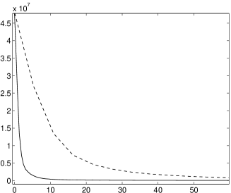
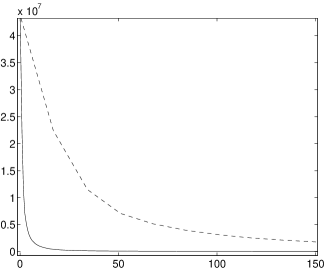
Figure 1: Convergence profiles of the Algorithm 2 (dotted line) and Algorithm 3 (solid line) versus computation time in seconds for a $3\times 3$ uniform blur (left) and a $7\times 7$ uniform blur (right) and a $128\times 128$-image.

It can be noticed that the larger the kernel blur size is, the higher the gain is. This is due to the fact that the number of proximity operators to compute increases with the kernel size.

5.2.2 Comparison between different forms of total variation

In Section 3.3, we have introduced the proximity operator associated with discretized total variation functions and the possibility of choosing various filters has been mentioned. In Figure 2, tests have been carried out on “Peppers” degraded by a $3\times 3$ uniform blur and corrupted by Poisson noise with scaling parameter $\alpha=0.1$. We compare the restored images for different kinds of total variation, in terms of Signal to Noise Ratio – SNR and structural similarity measure – SSIM [65]. The SSIM takes a value between -1 to 1, the maximum value being obtained for two identical images. Each curve represents the resulting SNR and SSIM versus $\mu$ (the regularization parameter related to the total variation), for a given form of $\mathrm{tv}$ (i.e. a given filter associated with either an isotropic or anisotropic function $\rho_{\mathrm{tv}}$). A small wavelet regularization parameter $\vartheta=10^{-3}$ has been chosen in order to better illustrate the influence of the different $\mathrm{tv}$ forms on restoration quality.

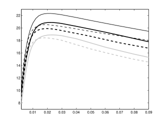
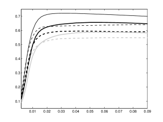
Figure 2: SNR (left) and SSIM (right) for different total variation terms with respect to $\mu$. Roberts: thin-black line, Finite difference: thick-black, Prewitt: thick-gray, $\rho_{\mathrm{tv}}=\sqrt{|\cdot|^{2}+|\cdot|^{2}}$: solid line and $\rho_{\mathrm{tv}}=|\cdot|+|\cdot|$: dashed line

It can be concluded from Figure 2 that the choice of the gradient filters and of the form (isotropic/anisotropic) of $\rho_{\mathrm{tv}}$ has a significant influence on the restoration quality when the wavelet regularization is small. However, we also noticed in our numerical experiments that when the wavelet regularization parameter $\vartheta$ becomes larger, the choice of the $\mathrm{tv}$ form has a lower influence on the restoration quality provided that the regularization parameters are appropriately chosen.

5.2.3 Boundary effects on restored images

This section illustrates the influence of boundary effect processing. More precisely, we degraded an extended version of “Boat” image by a $7\times 7$ uniform blur, and the resulting blurred image was cropped to create an image of size $256\times 256$. As a consequence, the boundary values are functions of pixel locations which are no longer present in the blurred image. The scaling parameter associated with Poisson noise is $\alpha=0.5$. The objective is then to restore the image (which was centered) by using one of the convolution models discussed in Section 3.2, namely either a periodic convolution or a convolution with zero-padding. Visual and quantitative results are given in Figure 3.

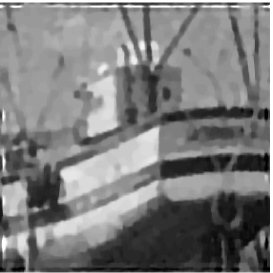
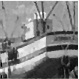
SNR = $16.9$ dB - SSIM = $0.62$	SNR = $17.7$ dB - SSIM = $0.64$

Figure 3: Periodic (left) and zero-padded (right) restoration.

As it can be noticed from this figure, the periodic convolution model introduces significant boundary artefacts unlike the convolution with zero-padding. The results obtained when considering “Peppers” led to the same conclusion. For “Sebal”, zero-padding or periodic models provided similar results.

5.2.4 Decimated convolution

We now present experimental results for a $256\times 256$ SPOT image degraded by a uniform decimated blur with a kernel size $Q=3\times 3$ and a decimated factor $d=2$. The scaling parameter of the Poisson noise is equal to $\alpha=1$. Due to the structure of the degradation operator, the data fidelity is splitted in a sum of $I=4$ functions. The results are presented in Figure 4 where the good behaviour of the model can be observed.

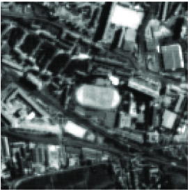
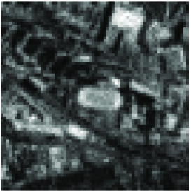
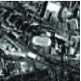
Original	Degraded	Restored $(\vartheta=1,\mu=10^{-3})$
		SNR = 16.1 - SSIM = 0.79

Figure 4: Restoration results for “Spot” image.

5.2.5 Influence of each regularization term

We now present numerical and visual results for the different kinds of regularization when a generalized Kullback-Leibler divergence is used as a data fidelity term. This experiment allows us to compare the hybrid regularization with existing approaches based on a wavelet-frame [44] regularization or a total variation regularization [43, 44]. The latter regularized solutions can be computed either by using augmented Lagrangian techniques [43, 44] or with our splitting approach (by setting $\vartheta=0$ or $\mu=0$). In our experiments, the computation time of the two approaches was observed to be similar. Note that comparisons performed in [44] led to the conclusion that the wavelet-frame regularization is quite competitive with respect to other existing restoration methods [38].

In the images displayed in Figures 5, 6, and 7, one can observe the artefacts related to the wavelet regularization, the staircase effects which are typical of the total variation penalization, some checkerboard patterns resulting of the chosen gradient discretization, and also the benefits which can be drawn from the use of a hybrid regularization.

Similarly to [44], the values of $\mu$ and $\vartheta$ have been adjusted so as to maximize the SNR. Optimizing the hyperparameters manually as we did is a common practice in imaging applications, especially when a data set of test images having similar characteristics as the one to be restored (medical images, satellite images,…) is available. Automatic methods for the optimization of the hyperparameters can also be found in the literature such as cross-validation [66], Stochastic EM [67], MCMC [68, 69] or Stein-based methods [70]. These automatic procedures often are relatively intensive. They will not be addressed in this paper due to the lack of space.

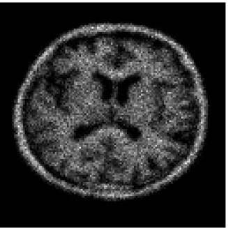
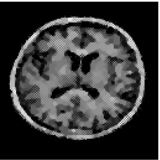
Degraded, $\alpha=0.1$ and uniform blur $3\times 3$	Total variation regularization
SNR = 8.88 dB - SSIM = 0.69	SNR = 11.2 dB - SSIM = 0.79
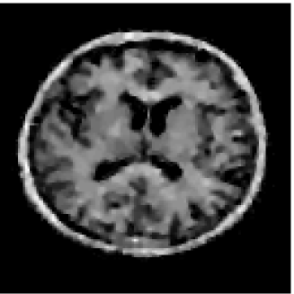
Hybrid regularization $(\vartheta=0.09,\mu=0.006)$	Wavelet-frame regularization
SNR= 12.4 dB - SSIM= 0.85	SNR= 11.7 dB - SSIM= 0.83

Figure 5: Restoration results for “Sebal” image.

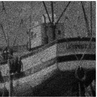
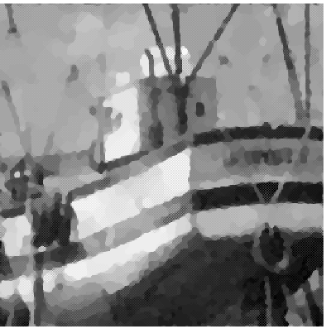
Degraded, $\alpha=0.1$ and uniform blur $3\times 3$	Total variation regularization
SNR = 11.2 dB - SSIM = 0.27	SNR = 17.8 dB - SSIM = 0.60
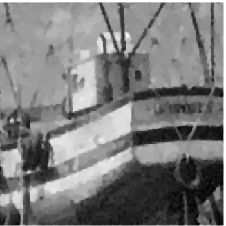
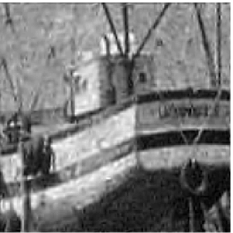
Hybrid regularization $(\vartheta=0.06,\mu=0.011)$	Wavelet-frame regularization
SNR=18.8 dB - SSIM=0.67	SNR=18.0 dB - SSIM= 0.62

Figure 6: Restoration results for “Boat” image.

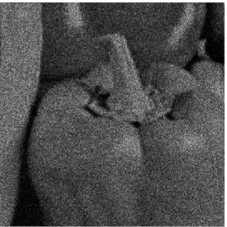
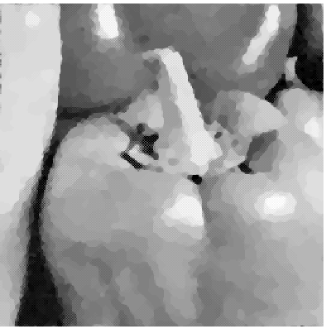
Degraded, $\alpha=0.1$ and uniform blur $3\times 3$	Total variation regularization
SNR = 11.4 dB - SSIM = 0.16	SNR = 22.1 dB - SSIM = 0.69
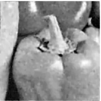
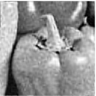
Hybrid regularization $(\vartheta=0.2,\mu=0.006)$	Wavelet-frame regularization
SNR = 22.7 dB - SSIM = 0.74	SNR= 21.4 dB - SSIM = 0.68

Figure 7: Restoration results for “Peppers” image.

6 Conclusion

A new convex regularization approach to restore data degraded by a (possibly decimated) convolution operator and a non necessarily additive noise has been proposed. The main advantages of the method are (i) to deal directly with the “true” noise likelihood (i.e. the Kullback-Leibler divergence in the case of Poisson noise) without requiring any approximation of it; (ii) to permit the use of sophisticated regularization functions, e.g. one promoting sparsity in a wavelet frame domain and a total variation penalization. In addition, the proposed algorithm has a parallel structure which makes it easily implementable on multicore architectures. Numerical and visual results demonstrate the effectiveness of the proposed approach. One can note that, even if the paper is devoted to the case of convolutive operators, this approach could be generalized to more general linear operators.

Note that the primal-dual approaches [71, 72, 73, 74, 75] can offer alternative solutions to the ones developed in this paper. However, one of the advantages of PPXA is that it easily leads to efficient parallel implementations

7 Proof of Proposition 3.4

Since $D=LL^{\top}$ is the matrix associated with a bijective operator, $L$ is associated with a surjective one and $\mathrm{dom}\,\Upsilon\neq\varnothing\Rightarrow\mathrm{dom}\,(\Upsilon\circ L)\neq\varnothing$. This allows us to conclude that $h=\Upsilon\circ L$ is a function of $\Gamma_{0}(\mathbb{R}^{X})$.
To calculate the proximity operator of $h$, we now come back to the definition of this operator. We have thus, for every $w\in\mathbb{R}^{X}$,

$$\mathrm{prox}_{h}w=\arg\min_{v\in\mathbb{R}^{X}}\frac{1}{2}\|v-w\|^{2}+\Upsilon(Lv).$$ (45)

We can write any vector $v\in\mathbb{R}^{X}$ as a sum of an element $L^{\top}t\in\mathrm{ran}\,L^{\top}$ and $v_{\perp}\in(\mathrm{ran}\,L^{\top})^{\perp}=\ker L$. We have then $Lv=LL^{\top}t=Dt$. Similarly, we can write $w=L^{\top}u+w_{\perp}$ where $u\in\mathbb{R}^{Y}$ and $w_{\perp}\in\ker L$. So, $\mathrm{prox}_{h}w$ can be determined by finding

$$\min_{(t,v_{\perp})\in\mathbb{R}^{Y}\times\mathbb{R}^{X}}\frac{1}{2}\|L^{\top}t+v_{\perp}-L^{\top}u-w_{\perp}\|^{2}+\Upsilon(Dt)\\ =\min_{(t,v_{\perp})\in\mathbb{R}^{Y}\times\mathbb{R}^{X}}\frac{1}{2}\|L^{\top}(t-u)\|^{2}+\frac{1}{2}\|v_{\perp}-w_{\perp}\|^{2}+\Upsilon(Dt).$$ (46)

This yields

$$v_{\perp}=w_{\perp}=w-L^{\top}u$$ (47)

and it remains to find

$$\min_{t\in\mathbb{R}^{Y}}\frac{1}{2}\|L^{\top}(t-u)\|^{2}+\Upsilon(Dt)=\min_{t\in\mathbb{R}^{Y}}\frac{1}{2}{(t-u)}^{\top}{D(t-u)}+\Upsilon(Dt).$$ (48)

By using the separability of $\Upsilon$, this is equivalent to finding

$$\min_{t\in\mathbb{R}^{Y}}\sum_{m=1}^{Y}\frac{1}{2}\Delta_{m}({o_{m}}^{\top}{t}-{o_{m}}^{\top}{u})^{2}+\psi_{m}(\Delta_{m}{o_{m}}^{\top}{t}).$$ (49)

It can be deduced from [23, Lemma 2.6] that, for every $m\in\{1,\ldots,Y\}$,

$${o_{m}}^{\top}{t} =\mathrm{prox}_{\frac{1}{\Delta_{m}}\psi_{m}(\Delta_{m}\cdot)}({o_{m}}^{\top}{u})$$

$$=\frac{1}{\Delta_{m}}\mathrm{prox}_{\Delta_{m}\psi_{m}}(\Delta_{m}\,{o_{m}}^{\top}{u}),$$ (50)

which, according to [26, Proposition 2.10], leads to

$$t =D^{-1}\sum_{m=1}^{Y}\mathrm{prox}_{\Delta_{m}\psi_{m}}(\Delta_{m}{o_{m}}^{\top}{u})\,o_{m}$$

$$=D^{-1}\mathrm{prox}_{D\Upsilon}(Du).$$ (51)

Altogether, (47) and (7) yield

$$v=w+L^{\top}\big{(}D^{-1}\mathrm{prox}_{D\Upsilon}(Du)-u\big{)}.$$

In addition, since $L^{\top}u$ is the projection of $w$ onto $\mathrm{ran}\,L^{\top}$, $u=(LL^{\top})^{-1}Lw=D^{-1}Lw$ and (17) follows.

8 Proof of Proposition 3.8

By using the proximity operator definition (7),

$$\pi=\mathrm{prox}_{\mu\mathrm{tv}_{p_{1},p_{2}}}(y)$$

minimizes

$$\frac{1}{2}\|\pi- y\|^{2}+\mu\mathrm{tv}_{p_{1},p_{2}}(\pi)$$

$$= \;\frac{1}{2}\sum_{(n_{1},n_{2})\in\mathbb{B}}(\pi_{n_{1},n_{2}}-y_{n_{1},n_{2}})^{2}$$

$$+\sum_{n_{1}=0}^{\lfloor\frac{N_{1}-p_{1}}{P_{1}}\rfloor-1}\sum_{n_{2}=0}^{\lfloor\frac{N_{2}-p_{2}}{P_{2}}\rfloor-1}\Big{\{}\frac{1}{2}\|\Pi_{n_{1},n_{2}}^{p_{1},p_{2}}-Y_{n_{1},n_{2}}^{p_{1},p_{2}}\|^{2}_{\rm F}+\mu\;\rho_{\rm tv}\big{(}\mathrm{tr}(H^{\top}\Pi_{n_{1},n_{2}}^{p_{1},p_{2}}),\mathrm{tr}(V^{\top}\Pi_{n_{1},n_{2}}^{p_{1},p_{2}})\big{)}\Big{\}}$$ (52)

where $\|\cdot\|_{\rm F}$ denotes the Frobenius norm, for every $(n_{1},n_{2})\in\{0,\ldots,\lfloor\frac{N_{1}-p_{1}}{P_{1}}\rfloor-1\}\times\{0,\ldots,\lfloor\frac{N_{2}-p_{2}}{P_{2}}\rfloor-1\}$,

$$\Pi_{n_{1},n_{2}}^{p_{1},p_{2}}=(\pi_{P_{1}n_{1}+p_{1}+p_{1}^{\prime},P_{2}n_{2}+p_{2}+p_{2}^{\prime}})_{0\leq p_{1}^{\prime}<P_{1},0\leq p_{2}^{\prime}<P_{2}}$$ (53)

and

$$\mathbb{B}=\{(n_{1},n_{2})\in\mathbb{N}^{2}\mid\; 0\leq n_{1}<p_{1}\;\text{or}\;0\leq n_{2}<p_{2}\;$$

$$\text{or}\;P_{1}\lfloor\frac{N_{1}-p_{1}}{P_{1}}\rfloor\leq n_{1}<N_{1}\;$$

$$\text{or}\;P_{2}\lfloor\frac{N_{2}-p_{2}}{P_{2}}\rfloor\leq n_{2}<N_{2}\}.$$ (54)

It is then clear that (38) holds since the variables $\pi_{n_{1},n_{2}}$ with $(n_{1},n_{2})\in\mathbb{B}$ are not elements of the matrices $\Pi_{n_{1},n_{2}}^{p_{1},p_{2}}$ with $n_{1}\in\{0,\ldots,\lfloor\frac{N_{1}-p_{1}}{P_{1}}\rfloor-1\}$ and $n_{2}\in\{0,\ldots,\lfloor\frac{N_{2}-p_{2}}{P_{2}}\rfloor-1\}$. In addition, since it has been assumed that $\mathrm{tr}(H^{\top}V)=0$ and $\|H\|_{\rm F}=\|V\|_{\rm F}=1$, the matrices $\Pi_{n_{1},n_{2}}^{p_{1},p_{2}}$ and $Y_{n_{1},n_{2}}^{p_{1},p_{2}}$ can be decomposed in an orthogonal manner as follows:

$$\begin{cases}\Pi_{n_{1},n_{2}}^{p_{1},p_{2}}=\beta_{n_{1},n_{2}}^{p_{1},p_{2}}H+\kappa_{n_{1},n_{2}}^{p_{1},p_{2}}V+(\Pi_{n_{1},n_{2}}^{p_{1},p_{2}})^{\perp}\\ Y_{n_{1},n_{2}}^{p_{1},p_{2}}=h_{n_{1},n_{2}}^{p_{1},p_{2}}H+v_{n_{1},n_{2}}^{p_{1},p_{2}}V+(Y_{n_{1},n_{2}}^{p_{1},p_{2}})^{\perp}\\ \end{cases}$$ (55)

where

$$\beta_{n_{1},n_{2}}^{p_{1},p_{2}} =\mathrm{tr}(H^{\top}\Pi_{n_{1},n_{2}}^{p_{1},p_{2}}),$$

$$\kappa_{n_{1},n_{2}}^{p_{1},p_{2}} =\mathrm{tr}(V^{\top}\Pi_{n_{1},n_{2}}^{p_{1},p_{2}}),$$ (56)

$$(\Pi_{n_{1},n_{2}}^{p_{1},p_{2}})^{\perp} =\Pi_{n_{1},n_{2}}^{p_{1},p_{2}}-\beta_{n_{1},n_{2}}^{p_{1},p_{2}}H-\kappa_{n_{1},n_{2}}^{p_{1},p_{2}}V,$$

$$(Y_{n_{1},n_{2}}^{p_{1},p_{2}})^{\perp} =Y_{n_{1},n_{2}}^{p_{1},p_{2}}-h_{n_{1},n_{2}}^{p_{1},p_{2}}H-v_{n_{1},n_{2}}^{p_{1},p_{2}}V,$$ (57)

and $(h_{n_{1},n_{2}}^{p_{1},p_{2}},v_{n_{1},n_{2}}^{p_{1},p_{2}})$ is given by (36). After some simplications, we have thus to minimize, for every $n_{1}\in\{0,\ldots,\lfloor\frac{N_{1}-p_{1}}{P_{1}}\rfloor-1\}$ and $n_{2}\in\{0,\ldots,\lfloor\frac{N_{2}-p_{2}}{P_{2}}\rfloor-1\}$,

$$\frac{1}{2} \|\Pi_{n_{1},n_{2}}^{p_{1},p_{2}}-Y_{n_{1},n_{2}}^{p_{1},p_{2}}\|^{2}_{\rm F}+\mu\;\rho_{\rm tv}\big{(}\mathrm{tr}(H^{\top}\Pi_{n_{1},n_{2}}^{p_{1},p_{2}}),\mathrm{tr}(V^{\top}\Pi_{n_{1},n_{2}}^{p_{1},p_{2}})\big{)}$$

$$=\frac{1}{2}\|(\Pi_{n_{1},n_{2}}^{p_{1},p_{2}})^{\perp}-(Y_{n_{1},n_{2}}^{p_{1},p_{2}})^{\perp}\|^{2}_{\rm F}$$

$$+\frac{1}{2}(\beta_{n_{1},n_{2}}^{p_{1},p_{2}}-h_{n_{1},n_{2}}^{p_{1},p_{2}})^{2}$$

$$+\frac{1}{2}(\kappa_{n_{1},n_{2}}^{p_{1},p_{2}}-v_{n_{1},n_{2}}^{p_{1},p_{2}})^{2}$$

$$+\mu\;\rho_{\rm tv}\big{(}\beta_{n_{1},n_{2}}^{p_{1},p_{2}},\kappa_{n_{1},n_{2}}^{p_{1},p_{2}}\big{)}.$$ (58)

This shows that (37) is satisfied and that $(\Pi_{n_{1},n_{2}}^{p_{1},p_{2}})^{\perp}=(Y_{n_{1},n_{2}}^{p_{1},p_{2}})^{\perp}.$ Eq. (35) straightforwardly follows.

9 Derivation of Algorithm 3

Let $\Pi_{F}$ denote the projector on $\mathrm{ran}\,F$. For every $u\in\mathbb{R}^{K}$, we have

$$u=\Pi_{F}u+u^{\perp}$$ (59)

where $u^{\perp}\in(\mathrm{ran}\,F)^{\perp}$ is the projection error and there exists $q\in\mathbb{R}^{N}$ such that

$$\Pi_{F}u=Fq.$$ (60)

By combining this with the fact that $F^{\top}u^{\perp}=0$, we obtain the relation,

$$q=\frac{1}{\nu}F^{\top}$$ (61)

which allows us to deduce from (59) that

$$u^{\perp}=u-\frac{1}{\nu}FF^{\top}u.$$

Now, consider the first step of Algorithm 2: $(\forall j\in\{1,\ldots,S\})$

$$p_{j,\ell}=u_{j,\ell}+\frac{F}{\nu}(\mathrm{prox}_{\nu\gamma g_{j}/\omega_{j}}(F^{\top}u_{j,\ell})-F^{\top}u_{j,\ell})+a_{j,\ell}$$ (62)

where $a_{j,\ell}$ is assumed to belong to $\mathrm{ran}\,F$, i.e. $a_{j,\ell}=F\widetilde{a}_{j,\ell}$ with $\widetilde{a}_{j,\ell}\in\mathbb{R}^{N}$. Defining $q_{j,\ell}\in\mathbb{R}^{N}$ similarly to (60) yields $\Pi_{F}p_{j,\ell}=Fq_{j,\ell}$. According to (61), $q_{j,\ell}$ is such that

$$q_{j,\ell}=\frac{1}{\nu}F^{\top}p_{j,\ell}.$$ (63)

By combining (62) and (63),

$$q_{j,\ell}=\frac{1}{\nu}\mathrm{prox}_{\nu\gamma g_{j}/\omega_{j}}(v_{j,\ell})+\widetilde{a}_{j,\ell}\qquad\mbox{where $v_{j,\ell}=F^{\top}u_{j,\ell}$}.$$ (64)

Moreover, since $p_{j,\ell}=Fq_{j,\ell}+p_{j,\ell}^{\perp}$, the computation of the variable $p_{\ell}=\sum_{j=1}^{J}\omega_{j}p_{j,\ell}$ in Algorithm 2 can be rewritten as

$$p_{\ell}=F\sum_{j=1}^{S}\omega_{j}q_{j,\ell}+\sum_{j=1}^{S}\omega_{j}p_{j,\ell}^{\perp}+\sum_{j=S+1}^{J}\omega_{j}p_{j,\ell}$$ (65)

where, according to (59), (60), (62) and (64),

$$p_{j,\ell}^{\perp}=u_{j,\ell}-\frac{1}{\nu}FF^{\top}u_{j,\ell}=u_{j,\ell}^{\perp}.$$ (66)

In the new formulation, the last steps of the algorithm consist of updating $u_{j,\ell}^{\perp}$ and $v_{j,\ell}$, for all $j\in\{1,\ldots,S\}$. We propose to define $r_{\ell}=2p_{\ell}-x_{\ell}$ , $\widetilde{r}_{\ell}=F^{\top}r_{\ell}$ and $r_{\ell}^{\perp}=r_{\ell}-\frac{1}{\nu}F\tilde{r}_{\ell}$, which yields $v_{j,\ell+1}=v_{j,\ell}+\lambda_{\ell}\big{(}\widetilde{r}_{\ell}-F^{\top}p_{j,\ell}\big{)}$ and $u_{j,\ell+1}^{\perp}=u_{j,\ell}^{\perp}+\lambda_{\ell}\big{(}r_{\ell}^{\perp}-p_{j,\ell}^{\perp}\big{)}$. By using (63) and (66), these relations can be simplified as

$$\begin{cases}v_{j,\ell+1}=v_{j,\ell}+\lambda_{\ell}\big{(}\widetilde{r}_{\ell}-\nu q_{j,\ell}\big{)}\\ \mbox{and}\\ u_{j,\ell+1}^{\perp}=u_{j,\ell}^{\perp}+\lambda_{\ell}\big{(}r_{\ell}^{\perp}-u_{j,\ell}^{\perp}\big{)},\end{cases}$$ (67)

which leads to Algorithm 3.
We finally note that Assumption 4.3 3) implies that Assumption 4.1 4) is satisfied since, for every $j\in\{1,\ldots,S\}$,

$$\sum_{\ell\in\mathbb{N}}\lambda_{\ell}\;\|a_{j,\ell}\|=\sum_{\ell\in\mathbb{N}}\lambda_{\ell}\;\|F\widetilde{a}_{j,\ell}\|\leq\|F\|\sum_{\ell\in\mathbb{N}}\lambda_{\ell}\;\|\widetilde{a}_{j,\ell}\|<+\infty.$$ (68)

This allows us to transpose the convergence results concerning Algorithm 2 to Algorithm 3.

References

- [1] N. Pustelnik, C. Chaux, and J.-C. Pesquet, “Hybrid regularization for data restoration in the presence of Poisson noise,” in Proc. Eur. Sig. and Image Proc. Conference, Glasgow, Scotland, Aug. 24-28 2009, pp. x+5.
- [2] L. M. Bregman, “The method of successive projection for a common point of convex sets,” Soviet Mathematics Doklady, vol. 6, pp. 688–692, 1965.
- [3] L. G. Gurin, B. T. Polyak, and E. V. Raik, “Projection methods for finding a common point of convex sets,” Zh. Vychisl. Mat. Mat. Fiz., vol. 7, pp. 1211–1228, 1967.
- [4] D. C. Youla and H. Webb, “Image restoration by the method of convex projections. Part I - theory,” IEEE Trans. on Medical Imaging, vol. 1, no. 2, pp. 81–94, Oct. 1982.
- [5] P. L. Combettes, “The foundations of set theoretic estimation,” Proceedings of the IEEE, vol. 81, no. 2, pp. 182–208, Feb. 1993.
- [6] P. L. Combettes, The Convex Feasibility Problem in Image Recovery, in vol. 95 of Advances in Imaging and Electron Physics, Academic Press, New York, 1996.
- [7] H. J. Trussell and M. R. Civanlar, “The feasible solution in signal restoration,” IEEE Trans. on Acous., Speech and Signal Proc., vol. 32, no. 2, pp. 201–212, Apr. 1984.
- [8] R. Gordon, R. Bender, and G. T. Herman, “Algebraic reconstruction techniques (ART) for three-dimensional electron microscopy and X-ray photography,” Journal of Theoretical Biology, vol. 29, no. 3, pp. 471–481, Dec. 1970.
- [9] A. N. Iusem and A. R. De Pierro, “Convergence results for an accelerated nonlinear Cimmino algorithm,” Numerische Mathematik, vol. 49, no. 4, pp. 367–378, Aug. 1986.
- [10] P. L. Combettes, “Inconsistent signal feasibility problems : least-squares solutions in a product space,” IEEE Trans. on Signal Proc., vol. 42, no. 11, pp. 2955–2966, Nov. 1994.
- [11] P. L. Combettes, “Convex set theoretic image recovery by extrapolated iterations of parallel subgradient projections,” IEEE Trans. on Image Proc., vol. 6, no. 4, pp. 493–506, Apr. 1997.
- [12] P. L. Combettes, “A block-iterative surrogate constraint splitting method for quadratic signal recovery,” IEEE Trans. on Signal Proc., vol. 51, no. 7, pp. 1771–1782, Jul. 2003.
- [13] J.-F. Aujol, “Some first-order algorithms for total variation based image restoration,” J. Math. Imag. Vis., vol. 34, no. 3, pp. 307–327, Jul. 2009.
- [14] S. Mallat, A wavelet tour of signal processing, Academic Press, San Diego, USA, 1997.
- [15] E. J. Candès and D. L. Donoho, “Recovering edges in ill-posed inverse problems: Optimality of curvelet frames,” Ann. Statist., vol. 30, no. 3, pp. 784–842, 2002.
- [16] E. Le Pennec and S. Mallat, “Sparse geometric image representations with bandelets,” IEEE Trans. on Image Proc., vol. 14, no. 4, pp. 423–438, Apr. 2005.
- [17] I. W. Selesnick, R. G. Baraniuk, and N. G. Kingsbury, “The dual-tree complex wavelet transform,” IEEE Signal Process. Mag., vol. 22, no. 6, pp. 123–151, Nov. 2005.
- [18] C. Chaux, L. Duval, and J.-C. Pesquet, “Image analysis using a dual-tree -band wavelet transform,” IEEE Trans. on Image Proc., vol. 15, no. 8, pp. 2397–2412, Aug. 2006.
- [19] I. Daubechies, M. Defrise, and C. De Mol, “An iterative thresholding algorithm for linear inverse problems with a sparsity constraint,” Comm. Pure Applied Math., vol. 57, no. 11, pp. 1413–1457, Nov. 2004.
- [20] M. A. T. Figueiredo and R. D. Nowak, “An EM algorithm for wavelet-based image restoration,” IEEE Trans. on Image Proc., vol. 12, no. 8, pp. 906–916, Aug. 2003.
- [21] J. Bect, L. Blanc-Féraud, G. Aubert, and A. Chambolle, “A -unified variational framework for image restoration,” in Proc. European Conference on Computer Vision, T. Pajdla and J. Matas, Eds., Prague, Czech Republic, May 2004, vol. LNCS 3024, pp. 1–13, Springer.
- [22] Z. Harmany, R. Marcia, and R. Willett, “This is SPIRAL-TAP: Sparse Poisson intensity reconstruction algorithms – theory and practice,” IEEE Trans. on Signal Proc., 2011, To appear, arXiv:1005.4274.
- [23] P. L. Combettes and V. R. Wajs, “Signal recovery by proximal forward-backward splitting,” Multiscale Modeling and Simulation, vol. 4, no. 4, pp. 1168–1200, Nov. 2005.
- [24] P. L. Combettes and J.-C. Pesquet, “Proximal splitting methods in signal processing,” in Fixed-Point Algorithms for Inverse Problems in Science and Engineering, H. H. Bauschke, R. Burachik, P. L. Combettes, V. Elser, D. R. Luke, and H. Wolkowicz, Eds., pp. 185–212. Springer-Verlag, New York, 2010.
- [25] J. J. Moreau, “Proximité et dualité dans un espace hilbertien,” Bull. Soc. Math. France, vol. 93, pp. 273–299, 1965.
- [26] C. Chaux, P. L. Combettes, J.-C. Pesquet, and V. R. Wajs, “A variational formulation for frame-based inverse problems,” Inverse Problems, vol. 23, no. 4, pp. 1495–1518, Jun. 2007.
- [27] J. M. Bioucas-Dias and M. A. T. Figueiredo, “A new TwIST: two-step iterative shrinkage/thresholding algorithms for image restoration,” IEEE Trans. on Image Proc., vol. 16, no. 12, pp. 2992–3004, Dec 2007.
- [28] A. Beck and M. Teboulle, “A fast iterative shrinkage-thresholding algorithm for linear inverse problems,” SIAM J. Imag. Sc., vol. 2, no. 1, pp. 183–202, 2009.
- [29] D. L. Donoho, “De-noising by soft-thresholding,” IEEE Trans. on Inform. Theory, vol. 41, no. 3, pp. 613–627, May 1995.
- [30] P. L. Combettes and J.-C Pesquet, “Proximal thresholding algorithm for minimization over orthonormal bases,” SIAM J. Optim., vol. 18, no. 4, pp. 1351–1376, Nov. 2007.
- [31] P. L. Lions and B. Mercier, “Splitting algorithms for the sum of two nonlinear operators,” SIAM J. Numer. Anal., vol. 16, no. 6, pp. 964–979, Dec. 1979.
- [32] J. Douglas and H. H. Rachford, “On the numerical solution of the heat conduction problem in two and three space variables,” Trans. Amer. Math. Soc., vol. 82, no. 2, pp. 421–439, Jul. 1956.
- [33] J. Eckstein and D. P. Bertsekas, “On the Douglas-Rachford splitting methods and the proximal point algorithm for maximal monotone operators,” Math. Programming, vol. 55, no. 3, pp. 293–318, Jun. 1992.
- [34] P. L. Combettes and J.-C. Pesquet, “A Douglas-Rachford splitting approach to nonsmooth convex variational signal recovery,” IEEE J. Select. Topics in Sig. Proc., vol. 1, no. 4, pp. 564–574, Dec. 2007.
- [35] P. L. Combettes and J.-C. Pesquet, “A proximal decomposition method for solving convex variational inverse problems,” Inverse Problems, vol. 24, no. 6, pp. x+27, Dec. 2008.
- [36] M. Fornasier, “Domain decomposition methods for linear inverse problems with sparsity constraints,” Inverse Problems, vol. 23, pp. 2505–2526, 2007.
- [37] M. Fornasier and C.-B. Schönlieb, “Subspace correction methods for total variation and -minimization,” SIAM J. Numer. Anal., vol. 47, no. 8, pp. 3397–3428, 2009.
- [38] F.-X. Dupé, M. J. Fadili, and J.-L. Starck, “A proximal iteration for deconvolving Poisson noisy images using sparse representations,” IEEE Trans. on Image Proc., vol. 18, no. 2, pp. 310–321, Feb. 2009.
- [39] C. Chaux, J.-C. Pesquet, and N. Pustelnik, “Nested iterative algorithms for convex constrained image recovery problems,” SIAM J. Imag. Sc., vol. 2, no. 2, pp. 730–762, Jun. 2009.
- [40] M. R. Hestenes, “Multiplier and gradient methods,” Journal of Opt. Theory and Appli., vol. 4, no. 5, pp. 303–320, Nov. 1969.
- [41] M. Fortin and R. Glowinski, Eds., Augmented Lagrangian Methods: Applications to the Numerical Solution of Boundary-Value Problems, Elsevier Science Ltd, Amsterdam: North-Holland, 1983.
- [42] T. Goldstein and S. Osher, “The split Bregman method for regularized problems,” SIAM J. Imag. Sc., vol. 2, no. 2, pp. 323–343, 2009.
- [43] S. Setzer, G. Steidl, and T. Teuber, “Deblurring Poissonian images by split Bregman techniques,” Journal of Visual Comm. and Image Repres., vol. 21, no. 3, pp. 193–199, Apr. 2010.
- [44] M. A. T. Figueiredo and J. M. Bioucas-Dias, “Restoration of Poissonian images using alternating direction optimization,” IEEE Trans. on Image Proc., vol. 19, no. 12, pp. 3133–3145, Dec. 2010.
- [45] B. He, M. Tao, and X. Yuan, “A splitting method for separate convex programming with linking linear constraints,” Tech. Rep., 2011, http://www.optimization-online.org/DB_FILE/2010/06/2665.pdf.
- [46] J. Bioucas-Dias and M. A. T. Figueiredo, “An iterative algorithm for linear inverse problems with compound regularizers,” in Proc. Int. Conf. on Image Proces., San Diego, CA, USA, Oct. 12–15 2008, pp. 685–688.
- [47] Y.-W. Wen, M. K. Ng, and W.-K. Ching, “Iterative algorithms based on decoupling of deblurring and denoising for image restoration,” SIAM J. on Scientific Computing, vol. 30, no. 5, pp. 2655–2674, 2008.
- [48] I. Daubechies, Ten lectures on wavelets, Society for Industrial and Applied Mathematics, Philadelphia, PA, 1992.
- [49] M. N. Do and M. Vetterli, “The contourlet transform: an efficient directional multiresolution image representation,” IEEE Trans. on Image Proc., vol. 14, no. 12, pp. 2091–2106, Dec. 2005.
- [50] D. Han and D. R. Larson, “Frames, bases, and group representations,” Mem. Amer. Math. Soc., vol. 147, no. 697, pp. x+94, 2000.
- [51] M. N. Do and M. Vetterli, “Wavelet-based texture retrieval using generalized Gaussian density and Kullback-Leibler distance,” IEEE Trans. on Image Proc., vol. 11, no. 2, pp. 146–158, Feb. 2002.
- [52] J. J. Moreau, “Fonctions convexes duales et points proximaux dans un espace hilbertien,” C. R. Acad. Sci., vol. 255, pp. 2897–2899, 1962.
- [53] D. Titterington, “On the iterative image space reconstruction algorithm for ECT,” IEEE Trans. on Medical Imaging, vol. 6, no. 1, pp. 52–56, Mar. 1987.
- [54] G. H. Golub and C. F. Van Loan, Matrix computations, The Johns Hopkins University Press; 3rd edition, 1996.
- [55] L. Rudin, S. Osher, and E. Fatemi, “Nonlinear total variation based noise removal algorithms,” Physica D, vol. 60, no. 1-4, pp. 259–268, Nov. 1992.
- [56] L. Rudin and S. Osher, “Total variation based image restoration with free local constraints,” in Proc. Int. Conf. on Image Proces., Austin, Texas, USA, Nov. 13-16 1994, vol. 1, pp. 31–35.
- [57] F. Malgouyres, “Mathematical analysis of a model which combines total variation and wavelet for image restoration,” Journal of information processes, vol. 2, no. 1, pp. 1–10, 2002.
- [58] J.-F. Aujol, G. Gilboa, T. Chan, and S. Osher, “Structure-texture image decomposition - modeling, algorithms, and parameter selection,” International Journal of Computer Vision, vol. 67, no. 1, pp. 111–136, Apr. 2006.
- [59] P. Weiss, L. Blanc-Féraud, and G. Aubert, “Efficient schemes for total variation minimization under constraints in image processing,” SIAM J. on Scientific Computing, vol. 31, no. 3, pp. 2047–2080, Apr. 2009.
- [60] X. Bresson and T.F. Chan, “Fast dual minimization of the vectorial total variation norm and applications to color image processing,” Inverse Problems and Imaging, vol. 2, pp. 455–484, 2008.
- [61] A. Chambolle, “An algorithm for total variation minimization and applications,” J. Math. Imag. Vis., vol. 20, no. 1-2, pp. 89–97, Jan. 2004.
- [62] J. A. Fessler, “Hybrid Poisson/polynomial objective functions for tomographic image reconstruction from transmission scans,” IEEE Trans. on Image Proc., vol. 4, no. 10, pp. 1439–1450, Oct. 1995.
- [63] J. Zheng, S. S. Saquib, K. Sauer, and C. A Bouman, “Parallelizable bayesian tomography algorithms with rapid, guaranteed convergence,” IEEE Trans. on Image Proc., vol. 9, no. 10, pp. 1745–1759, Oct. 2000.
- [64] E. Chouzenoux, S. Moussaoui, and J. Idier, “Majorize-minimize linesearch for inversion methods involving barrier function optimization,” Inverse Problems, Submitted 2011.
- [65] Z. Wang and A. C. Bovik, “Mean squared error: love it or leave it?,” IEEE Signal Process. Mag., vol. 26, no. 1, pp. 98–117, Jan. 2009.
- [66] N. P. Galatsanos and A. K. Katsaggelos, “Methods for choosing the regularization parameter and estimating the noise variance in image restoration and their relation,” IEEE Trans. on Image Proc., vol. 1, no. 3, pp. 322–336, Jul. 1992.
- [67] B. Delyon, M. Lavielle, and E. Moulines, “Convergence of a stochastic approximation version of the EM algorithm,” Ann. Statist., vol. 27, no. 1, pp. 94–128, 1999.
- [68] C. Robert and G. Casella, Monte Carlo statistical methods, Springer, New York, 2004.
- [69] L. Chaâri, J.-C. Pesquet, J.-Y. Tourneret, P. Ciuciu, and A. Benazza-Benyahia, “A hierarchical bayesian model for frame representation,” IEEE Trans. on Signal Proc., vol. 58, no. 11, pp. 5560–5571, Nov. 2010.
- [70] S. Ramani, T. Blu, and M. Unser, “Monte-Carlo SURE: A black-box optimization of regularization parameters for general denoising algorithms,” IEEE Trans. on Image Proc., vol. 17, no. 9, pp. 1540–1554, Sep. 2008.
- [71] M. Zhu and T.F. Chan, “An efficient primal-dual hybrid gradient algorithm for total variation image restoration,” UCLA CAM Report, 08–34, 2008.
- [72] X. Zhang, M. Burger, and S. Osher, “A unified primal-dual algorithm framework based on Bregman iteration,” Journal of Scientific Computing, vol. 46, no. 1, pp. 20–46, 2010.
- [73] E. Esser, X. Zhang, and T. Chan, “A general framework for a class of first order primal-dual algorithms for convex optimization in imaging science,” SIAM J. Imaging Sci., vol. 3, no. 4, pp. 1015–1046, 2010.
- [74] S. Setzer, G. Steidl, and T. Teuber, “Infimal convolution regularizations with discrete -type functionals,” Communications in Mathematical Sciences, 2010, http://kiwi.math.uni-mannheim.de/PAPERS/general_inf_conv_revised.pdf.
- [75] A. Chambolle and T. Pock, “A first-order primal-dual algorithm for convex problems with applications to imaging,” J. Math. Imag. Vis., vol. 40, no. 1, pp. 120–145, 2011.