Kink ratchets in the Klein-Gordon lattice free of the Peierls-Nabarro potential

Abstract

A discrete Klein-Gordon model with asymmetric potential that supports kinks free of the Peierls-Nabarro potential (PNp) is constructed. Undamped ratchet of kinks under harmonic AC driving force is investigated in this model numerically and contrasted with the kink ratchets in the conventional discrete model where kinks experience the PNp. We show that the PNp-free kinks exhibit ratchet dynamics very much different from that reported for the conventional lattice kinks which experience PNp [see, e.g., Phys. Rev. E 73, 066621 (2006)]. Particularly, we could not observe any significant influence of the discreteness parameter on the acceleration of PNp-free kinks induced by the AC driving.

I Introduction

Ratchet dynamics of a point-like particle or a quasi-particle such as soliton is the motion of the particle in a certain direction under AC force whose average is zero. Ratchet transport phenomenon can be observed under the following two conditions: (i) the system must be out of thermal equilibrium and (ii) the space-time symmetry of the system must be violated BraunKivshar:2004 ; FYZ:2000 ; Reimann:2001 ; Reimann:2002 . Ratchet dynamics has been receiving growing attention of researchers from different fields ranging from biology Cell:2002 ; Genetics:2008 and molecular motors Motors ; Motors1 ; Motors2 ; Motors3 ; Motors4 , through superconducting Josephson juctions JJ ; JJ1 ; JJ2 ; JJ3 and nonlinear optics OptLett:2006 , to Bose-Einstein condensate BEC:2008 and solid state physics SSP:2008 .

Soliton ratchets were first studied by Marchesoni Marchesoni:1996 for the overdamped Klein-Gordon equation. Unlike point-like particles, solitons can have internal vibrational modes IntModes and these modes can strongly affect the ratchet dynamics especially for underdamped case Modes1 ; Modes2 . So far, ratchet dynamics have been studied for a number of continuum soliton bearing systems Marchesoni:1996 ; Modes1 ; Modes2 ; Cont1 ; Cont2 ; Cont3 ; Cont4 ; Cont5 ; Cont6 , while in many applications ratchet was observed for discrete kinks JJ1 ; JJ2 ; JJ3 ; OptLett:2006 . Effects of discreteness on kink ratchets have been studied by Zolotaryuk and Salerno Discrete1 . They have found that in comparison with the continuum case, the discrete case shows a number of new features: nonzero depinning threshold for the driving amplitude, locking to the rational fractions of the driving frequency, and diffusive ratchet motion in the case of weak intersite coupling. For the damped, driven Frenkel-Kontorova chain, which is the discrete analog of the sine-Gordon equation, Martinez and Chacon have shown that phase disorder introduced into the asymmetric periodic driving force can enhance the ratchet effect Discrete2 .

In discrete systems translational invariance is typically lost and static solitary waves usually cannot be placed arbitrarily with respect to the lattice but only in the positions corresponding to the extremums of the Peirls-Nabarro potential (PNp), induced by the lattice. Configurations corresponding to the maximums of PNp are unstable while those corresponding to the minimums are stable. It has been found that the presence of PNp makes kink ratchets much more complicated in comparison to the continuum case Discrete1 .

On the other hand, in the recent past, several different families of discrete Klein-Gordon systems supporting translationally invariant static solutions with arbitrary shift along the lattice have been derived and investigated PhysicaD ; SpeightKleinGordon ; BenderTovbis ; JPA2005 ; Roy ; CKMS_PRE2005 ; BOP ; DKY_JPA_2006Mom ; oxt1 ; DKYF_PRE2006 ; Coulomb ; DKKS2007_BOP ; ArXivKDS ; SpeedyKinks ; BarHeerden . Such discrete models are often called exceptional. Physical properties of solitary waves in the exceptional discrete models were found to be very much different from their conventional counterparts. For instance, they can support conservation of momentum PhysicaD ; DKY_JPA_2006Mom and can support kinks which move with a special SpeedyKinks or arbitrary BarHeerden velocity without emitting radiation. Peculiarities of kink collisions in such models have been investigated in the work Roy . Static solutions in the exceptional discrete systems possess the translational Goldstone mode JPA2005 ; Roy . This means that such static solutions are not trapped by the lattice and can be accelerated by arbitrary weak external field. Exceptional discrete models can describe physically meaningful systems Coulomb , that is why investigation of physical properties of such systems is very important.

In the present study we continue the investigation of physical properties of the exceptional discrete models that support static kinks free of PNp. The main goal of the study is to see how the special properties of the kinks can influence their undamped ratchet dynamics under single-harmonic driving.

In order to achieve this goal we need to construct an exceptional discrete Klein-Gordon model with asymmetric background potential. It is important that the constructed model be Hamiltonian, otherwise energy increase in the system can be observed even for small-amplitude driving with the frequency laying outside the phonon band.

The paper is organized in five Sections. In Sec. II, we describe two discrete, Hamiltonian Klein-Gordon systems, with and without PNp, having asymmetric on-site potential and having common continuum limit. In Sec. III, we compare the properties of static kinks in these two models and then in Sec. IV study kink ratchets mostly for the PNp-free model. Section V concludes the paper.

II Discrete Klein-Gordon models with asymmetric potential

II.1 General formulation

The Klein-Gordon field has the Hamiltonian

$$H=\frac{1}{2}\int_{-\infty}^{\infty}\left[\phi_{t}^{2}+\phi_{x}^{2}+2V(\phi)\right]dx\,,$$ (1)

where $\phi(x,t)$ is the unknown field and $V(\phi)$ is a given potential function. The corresponding equation of motion is

$$\phi_{tt}=\phi_{xx}-V^{\prime}(\phi)\,,$$ (2)

where $V^{\prime}(\phi)=dV/d\phi$.

Equation (2) will be discretized on the lattice $x=nh$, where $n=0,\pm 1,\pm 2...$, and $h$ is the lattice spacing. Traditional discretization of Eq. (2) is

$$\ddot{\phi}_{n}=\frac{1}{h^{2}}(\phi_{n-1}-2\phi_{n}+\phi_{n+1})-V^{\prime}(\phi_{n}).$$ (3)

Using the discretized first integral (DFI) approach offered in JPA2005 and developed in DKYF_PRE2006 one can construct a discrete model whose static version is an integrable map. Following this method we begin with the first integral of static Eq. (2), $\phi_{x}^{2}-2V(\phi)+C=0$, where $C$ is the integration constant. The first integral can also be taken in the following modified form JPA2005

$$v(x)\equiv\phi_{x}-\sqrt{2V(\phi)-C}=0\,.$$ (4)

Next step is to rewrite the Hamiltonian Eq. (1) in terms of $v(x)$ as follows

$$H=\frac{1}{2}\int_{-\infty}^{\infty}\Big{\{}\phi_{t}^{2}+\left[v(x)\right]^{2}+2\phi_{x}\sqrt{2V(\phi)-C}\Big{\}}dx\,,$$ (5)

where we omitted the constant term.

The first integral Eq. (4) can be discretized as follows

$$\tilde{v}(\phi_{n-1},\phi_{n})\equiv\frac{\phi_{n}-\phi_{n-1}}{h}-\sqrt{2V(\phi_{n-1},\phi_{n})-C}=0,$$ (6)

where we demand that $V(\phi_{n-1},\phi_{n})\rightarrow V(\phi)$ in the continuum limit ($h\rightarrow 0$). Thus we obtain the discrete version of the Hamiltonian Eq. (1)

$$H=\frac{1}{2}\sum_{n}\Big{\{}\dot{\phi}_{n}^{2}+\left[\tilde{v}(\phi_{n-1},\phi_{n})\right]^{2}$$

$$+2\frac{\phi_{n}-\phi_{n-1}}{h}\sqrt{2V(\phi_{n-1},\phi_{n})-C}\Big{\}}\,.$$ (7)

Final step is to discretize the background potential as suggested by Speight SpeightKleinGordon ,

$$\sqrt{2V\left({\phi_{n-1},\phi_{n}}\right)-C}=\frac{{G(\phi_{n})-G(\phi_{n-1})}}{{\phi_{n}-\phi_{n-1}}},$$

$${\rm where}\quad G^{\prime}\left(\phi\right)=\sqrt{2V(\phi)-C}.$$ (8)

With this choice the last term of the Hamiltonian Eq. (II.1) reduces to $(2/h)[G(\phi_{n})-G(\phi_{n-1})]$ and it disappears in the telescopic summation. Further, according to Eq. (II.1), the discretized first integral Eq. (6) assumes the form

$$v(\phi_{n-1},\phi_{n})=\frac{\phi_{n}-\phi_{n-1}}{h}-\frac{G(\phi_{n})-G(\phi_{n-1})}{\phi_{n}-\phi_{n-1}},$$ (9)

and the equations of motion derived from Eq. (II.1) with $\tilde{v}(\phi_{n-1},\phi_{n})=v(\phi_{n-1},\phi_{n})$ are

$$\ddot{\phi}_{n}=-v(\phi_{n-1},\phi_{n})\frac{\partial}{{\partial\phi_{n}}}v(\phi_{n-1},\phi_{n})$$

$$-v(\phi_{n},\phi_{n+1})\frac{\partial}{{\partial\phi_{n}}}v(\phi_{n},\phi_{n+1}).$$ (10)

Obviously, equilibrium static solutions of this model can be found from the two-point nonlinear map $v(\phi_{n-1},\phi_{n})=0$, where $v(\phi_{n-1},\phi_{n})$ is given by Eq. (9). Such solutions can be constructed iteratively starting from any admissible initial value $\phi_{n-1}$ or $\phi_{n}$, and thus, the PNp is absent for such family of equilibrium solutions.

II.2 Polynomial asymmetric potential

Klein-Gordon kink ratchets are possible if the on-site potential or the driving force or both are asymmetric. We study the kink ratchets under single-harmonic AC driving and thus, the on-site potential must be asymmetric.

We take $G^{\prime}$ in Eq. (II.1) in the form of the quartic polynomial function

$$G^{\prime}(\phi)=a\phi^{4}+b\phi^{2}+c\phi+d\,,$$ (11)

where the cubic term was not taken into account because it can always be removed by a proper shift $\phi\rightarrow\phi-\phi_{0}$. Then the on-site potential (with $C=0$) is

$$V(\phi)=\frac{1}{2}\left(a\phi^{4}+b\phi^{2}+c\phi+d\right)^{2}.$$ (12)

The simplest discrete Klein-Gordon model corresponding to this potential (will be referred to as DKGM1), according to Eq. (3), is

$$\ddot{\phi}_{n}=\frac{1}{h^{2}}\left(\phi_{n-1}-2\phi_{n}+\phi_{n+1}\right)$$

$$-\left(a\phi_{n}^{4}+b\phi_{n}^{2}+c\phi_{n}+d\right)\left(4a\phi_{n}^{3}+2b\phi_{n}+c\right),$$ (13)

and its Hamiltonian is

$$H_{1}=\frac{1}{2}\sum_{n}\Big{\{}\dot{\phi}_{n}^{2}+\frac{1}{h^{2}}(\phi_{n}-\phi_{n-1})^{2}$$

$$+\left(a\phi_{n}^{4}+b\phi_{n}^{2}+c\phi_{n}+d\right)^{2}\Big{\}}\,.$$ (14)

A more sophisticated discrete Klein-Gordon model (will be referred to as DKGM2) is defined by Eq. (II.1) with

$$v\left(\phi_{n-1},\phi_{n}\right)=\frac{\phi_{n}-\phi_{n-1}}{h}$$

$$-\frac{a}{5}\left(\phi_{n}^{4}+\phi_{n}^{3}\phi_{n-1}+\phi_{n}^{2}\phi_{n-1}^{2}+\phi_{n}\phi_{n-1}^{3}+\phi_{n-1}^{4}\right)$$

$$-\frac{b}{3}\left({\phi_{n}^{2}+\phi_{n}\phi_{n-1}+\phi_{n-1}^{2}}\right)-\frac{c}{2}\left({\phi_{n}+\phi_{n-1}}\right)-d,$$ (15)

which was found by substituting Eq. (11) after integrating into Eq. (9). This model has the Hamiltonian

$$H_{2}=\frac{1}{2}\sum_{n}\Big{\{}\dot{\phi}_{n}^{2}+\left[v(\phi_{n-1},\phi_{n})\right]^{2}\Big{\}}\,.$$ (16)

Figure 1: On-site potential Eq. (12) for $b=0$ and $a=-1$, $c=0$, $d=1$ (dashed line); $a=-0.83988$, $c=0.382925$, $d=0.860756$ (dash-dotted line); $a=-0.643049$, $c=0.626843$, $d=0.706344$ (solid line).

The asymmetry of the potential Eq. (12) is controlled by the parameter $c$ and for $c=0$ the potential is symmetric. The on-site potential Eq. (12) has four parameters. Let us fix the height of the potential barrier equal to 0.5, the distance between the two minima equal to 2. The asymmetry can be chosen by setting a value of $c$. There is still one free parameter and we will take $b=0$.

In Fig. 1 we plot the on-site potential Eq. (12) for $b=0$ and $a=-1$, $c=0$, $d=1$ (dashed line); $a=-0.83988$, $c=0.382925$, $d=0.860756$ (dash-dotted line); $a=-0.643049$, $c=0.626843$, $d=0.706344$ (solid line). One can see that the asymmetry of the potential increases with $c$.

The asymmetric potential supports two vacuum solutions, $\phi_{n}=\phi_{1}$ and $\phi_{n}=\phi_{2}$, where $\phi_{1}$ and $\phi_{2}$ are the coordinates of the two minima of the on-site potential. Small-amplitude phonon vibrations of the form $\phi_{n}\sim\exp[i(qn-\omega t)]$, where $q$ is the phonon wavenumber and $\omega$ is the phonon frequency, have different spectra for different vacuums.

Borders of the phonon bands for each vacuum can be found for DKGM2 from

$$\omega_{1}^{2}=28a^{2}\phi_{i}^{6}+30ab\phi_{i}^{4}+20ac\phi_{i}^{3}$$

$$+3\left({2b^{2}+4ad}\right)\phi_{i}^{2}+6bc\phi_{i}+c^{2}+2bd,$$ (17)

$$\omega_{2}^{2}=\frac{{28}}{{25}}a^{2}\phi_{i}^{6}+2ab\phi_{i}^{4}+\frac{4}{5}ac\phi_{i}^{3}$$

$$+6\left({\frac{{b^{2}}}{9}+\frac{2}{5}ad}\right)\phi_{i}^{2}+\frac{2}{3}bc\phi_{i}+\frac{2}{3}bd+\frac{4}{{h^{2}}},$$ (18)

where $j=1,2$ and $\omega_{1}$ ($\omega_{2}$) corresponds to $q=0$ ($q=\pi$).

For DKGM1 the borders corresponding to $q=0$ coincide with that for DKGM2, while the borders corresponding to $q=\pi$ are

$$\omega_{2}^{2}=28a^{2}\phi_{i}^{6}+30ab\phi_{i}^{4}+20ac\phi_{i}^{3}+$$

$$6\left({b^{2}+2ad}\right)\phi_{i}^{2}+6bc\phi_{i}+c^{2}+2bd+\frac{4}{{h^{2}}}.$$ (19)

Numerical results in this work will be obtained for the on-site potential with the parameters $a=-0.643049$, $b=0$, $c=0.626843$, $d=0.706344$ (shown by the solid line in Fig. 1). The potential has minima at $\phi_{1}=-0.768678$ and $\phi_{2}=1.231321$ and a maximum at $\phi_{\max}=0.62462$.

III Properties of static kinks in two lattices

Before we proceed with the we need to study the properties of the kinks in DKGM1 and DKGM2 because they will help us to interpret the results of the kink ratchet dynamics study.

Equilibrium static kink solutions for the DKGM1 can be found numerically while for DKGM2 they can be found iteratively using Eq. (II.2) for any initial value of $\phi_{n}$ (or $\phi_{n-1}$) lying between two minima of the on-site potential.

In the DKGM1 there exists only one stable static kink configuration [shown in Fig. 2 (a)], corresponding to the minimum of the PNp. Static kinks in the DKGM2 do not experience the PNp and they can be placed anywhere with respect to the lattice. A family of equilibrium kinks is presented in Fig. 2 (b). Kinks in both models have asymmetric shape because of the asymmetry of the on-site potential.

Figure 2: (a) Stable equilibrium kink in DKGM1 and (b) a family of equilibrium kinks in DKGM2. In both cases $h=0.6$. Dashed lines show the locations of minima of the on-site potential and the dash-dotted line the location of the maximum.

Figure 3: Kink’s internal mode frequencies as the functions of the discreteness parameter for (a) DKGM1 and (b) DKGM2. Dashed line shows the bottom edge of the phonon band. Model parameters (here and in the following): $a=-0.643049$, $b=0$, $c=0.626843$, $d=0.706344$.

Small-amplitude oscillation spectra for the chains containing a kink are presented in Fig. 3 for different values of the discreteness parameter $h$. Dashed horizontal line shows the lower edge of the phonon band which is the same for both DKGM1 and DKGM2 and can be found from Eq. (II.2) for $j=1$ (soft minimum). Presented spectra show the kink’s internal vibrational modes. Since both discrete models share the same continuum limit [defined by Eq. (2) and Eq. (12)], for small discreteness ($h<0.25$) their spectra are close. Kink in DKGM1 [see in (a)] possesses two internal modes, one of them is the destroyed translational mode (for small $h$ it approaches zero frequency). Kink in DKGM2 [see in (b)] possesses the zero-frequency translational mode for any $h$, and for $h>0.48$ two new internal modes appear. Note that the spectrum in (b) was calculated for the kink having a particle at the maximum of the on-site potential and the kink internal mode frequencies within the studied range of $h$ are only slightly dependent on the location of the kink with respect to the lattice. For example, maximal difference between the internal mode frequencies for different kink positions with respect to the lattice observed at $h=1$ is 0.9%.

IV Kink ratchets

To study kink ratchets we add to the right-hand sides of equations of motion Eq. (II.2) (DKGM1) and Eq. (II.1) (DKGM2) the harmonic external force

$$F(t)=A\cos(\Omega t+\varphi),$$ (20)

with the amplitude $A$, frequency $\Omega$, and initial phase $\varphi$.

The initial conditions are thus as follows: we have a static equilibrium kink and at $t=0$ the force Eq. (20) is turned ”on”.

Figure 4: (a) Kink motion in DKGM2 at $h=0.6$ for two different values of initial phase of driving force $\varphi$ at the same amplitude $A=0.04$ and frequency $\Omega=0.5$. Oscillating lines, presenting the kink coordinate as the functions of time, are fitted by the square parabolas. (b) Acceleration of the kink and (c) initial velocity of the kink as the functions of $\varphi$.

Figure 5: Same as in Fig. 4 but for DKGM1, where kink experiences PNp.

In contrast to the majority of studies on the soliton ratchets we study the kink ratchets in the models that include no viscosity terms. We thus restrict ourselves to the case of driving force with a small amplitude ($A\leq 0.04$) and with frequency lying outside the phonon band (more precisely, below the phonon spectrum), otherwise phonon modes will be excited and the analysis of kink ratchets will become more complicated. Study of the undamped ratchet makes it possible to directly measure the force driving the kink.

For the models with damping terms it is customary to measure the efficiency of ratchet by the averaged velocity of steady motion of the soliton. This is not applicable to our case and instead, we measure the acceleration of the kink, $a$. As it will be shown, this approach works well for DKGM2, which is the primary subject of present study. This is demonstrated by the numerical results presented in Fig. 4 where in (a) we show two examples of kink’s trajectories (lines oscillating with the frequency of driving force, $\Omega=0.5$) and the least-square fit to these lines by square parabola

$$x(t)=at^{2}+v_{0}t+x_{0},$$ (21)

where $a$ is the net acceleration of the kink and $v_{0}$, $x_{0}$ are the kink’s initial velocity and coordinate, respectively. One can see that kink’s trajectories are fitted very well by the square parabola, meaning that the motion of kink is uniformly accelerated within the studied time domain.

The two trajectories shown in Fig. 5(a) correspond to different initial phases $\varphi$ of the driving force Eq. (20), while all other parameters are same: $A=0.04$, $\Omega=0.5$, $h=0.6$. In the case of $\varphi=0$ kink does not get initial momentum (in this case $v_{0}=0$) while in the case of $\varphi=0.1\pi$ it does ($v_{0}\neq 0$). However, acceleration $a$ of the kink in both cases is nearly same. In the panels (b) and (c) of Fig. 5 we plot the acceleration $a$ and the initial velocity $v_{0}$ of the kink, respectively, as the functions of the initial phase of driving force, $\varphi$. It can be seen that $v_{0}$ changes noticeably with $\varphi$ but its average over $\varphi$ is zero. On the other hand, the acceleration of the kink is practically independent of $\varphi$ and in the rest of the paper we set $\varphi=0$.

We have also checked how the kink’s acceleration $a$ depends on the initial position of the static kink with respect to the lattice, $x_{0}$, and found that $a$ practically does not depend on $x_{0}$ for the chains with $h=0.3$, $h=0.6$, and $h=0.9$. Even for the largest studied value of $h=0.9$ the difference between $a$ measured for kinks with different $x_{0}$ was within the numerical error.

In Fig. 5 we show same as in Fig. 4 but for DKGM1 where kink experiences PNp. The results in this case are strikingly different. Kink’s trajectories are now irregular and their least-square fit by square parabola does not make much sense. Nevertheless, in the panels (b) and (c) we present the values of $a$ and $v_{0}$ obtained from such fit of trajectories corresponding to various $\varphi$. Both $a$ and $v_{0}$ vary irregularly. We thus conclude that presence of PNp largely affects the ratchet dynamics of kink in our settings. In contrast to the DKGM2, where PNp is absent, motion of kinks in DKGM1 is not uniformly accelerated, at least for the range of parameters studied in this work, i.e., for rather small amplitude $A$ of the driving force. This is true already at moderate degree of discreteness, $h=0.6$, and the influence of PNp increases with increase in $h$.

Now we turn back to the DKGM2 and study the influence of the driving force parameters $A$ and $\Omega$ and the discreteness parameter $h$ on the uniformly accelerated dynamics of the kink.

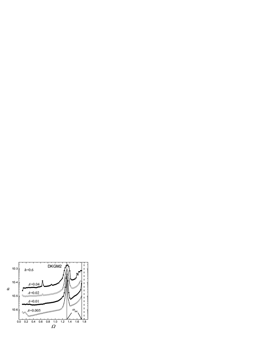
Figure 6: Acceleration of kink in DKGM2 as the function of frequency of driving force for different values of the force amplitude, $A$, as specified near each curve. Initial phase of the force $\varphi=0$ and the discreteness parameter $h=0.6$. Vertical solid lines show the frequencies of the kink’s internal modes and the vertical dashed line shows the lower edge of the phonon band.

Figure 7: Acceleration of kink in DKGM2 as the function of frequency of driving force for different values of the discreteness parameter $h$, as specified in each panel. Amplitude of the ac driving force is $A=0.04$ and initial phase of the force is $\varphi=0$. Vertical solid lines show the frequencies of the kink’s internal modes and the vertical dashed line shows the lower edge of the phonon band.

Results presented in Fig. 6 were obtained for $h=0.6$. Here we plot how the kink’s acceleration $a$ depends on the driving force frequency $\Omega$ at different values of the amplitude of the force $A$, as indicated near each curve. Vertical solid lines show the frequencies of the kink’s internal modes and the vertical dashed line shows the lower edge of the phonon band. It is readily seen that the acceleration of the kink increases by one or even two orders of magnitude (note the logarithmic scale for the ordinate) when the driving force frequency $\Omega$ approaches the frequency of kink’s internal mode $\omega_{\rm IM}=1.32$ (also note a smaller peak at $\omega_{\rm IM}/2$). This finding agrees well with earlier observations on the role of the kink’s internal modes on ratchet dynamics in the underdamped case BraunKivshar:2004 ; Modes1 ; Cont5 ; Cont6 ; Discrete1 . One can also see that $a$ increases when $\Omega$ approaches kink’s another internal mode frequency $\omega_{\rm IM}=1.73$. However, this increase can also be attributed to the fact that the phonon band edge ($\omega_{1}=1.795$) is also approached. A special investigation is required to clarify which of these two factors plays major role in increasing $a$. Looking at Fig. 6, one can also notice that the increase of the driving force amplitude $A$ by one order of magnitude has resulted in the increase in $a$ by two orders of magnitude and thus, $a\sim A^{2}$. Note that the scaling rule $\left\langle v\right\rangle\sim A^{2}$, where $\left\langle v\right\rangle$ is the averaged stationary kink velocity, has been reported for the soliton ratchets BraunKivshar:2004 .

Finally, we discuss the influence of the discreteness parameter $h$ on the kink’s acceleration $a$ at various driving force frequencies $\Omega$ (see Fig. 7). Here we set $A=0.04$ and consider the cases of relatively weak ($h=0.3$), moderate ($h=0.6$), and strong ($h=0.9$) discreteness. Again, vertical solid lines show the frequencies of the kink’s internal modes and the vertical dashed lines show the lower edge of the phonon band. Remarkably, for $\Omega<1.2$ the results are very close for all three values of $h$. This can be interpreted in such a way that for the discrete model supporting PNp-free kinks the ratchet dynamics is more like in the continuum case. The difference in the results that appears for $\Omega>1.2$ is related to the kink’s internal modes, whose frequencies are $h$-dependent [see Fig. 3(b)]. We note that there is no numerical data in Fig. 7(c) for $\Omega>1.325$. Above this frequency there is a mixed influence of the two kink’s internal modes and motion of the kink becomes different from uniformly accelerated so that one cannot assign any particular value of $a$ to it.

V Conclusions

Undamped ratchet dynamics of discrete Klein-Gordon kinks free of the Peirls-Nabarro potential was investigated numerically. For this purpose a lattice with asymmetric on-site potential was constructed.

It was found that, typically, in the presence of single-harmonic AC driving and in the absence of damping, PNp-free kink dynamics is uniformly accelerated until its velocity becomes too large and radiation losses start to contribute to the dynamics.

Our main finding is that discrete kink ratchets in the absence of PNp, at least for relatively small amplitude of driving force, is very much different from the conventional discrete kink ratchets experiencing PNp (compare the results plotted in Fig. 4 and Fig. 5).

Particularly, the acceleration of the PNp-free kink due to AC driving practically does not depend on $h$ in the non-resonance range of the driving frequency $\Omega$ (see Fig. 7). Indeed, in the range of $0.1<\Omega<1.2$ we have practically same $a(\Omega)$ dependence for relatively weak ($h=0.3$), moderate ($h=0.6$), and strong ($h=0.9$) discreteness. Is it is well-known that typically, physical properties of a discrete system are extremely sensitive to the discreteness parameter $h$. This unusual result can be explained by the fact that for the static kinks in DKGM2 PNp is precisely equal to zero.

Influence of $h$ on $a(\Omega)$ appears only through the influence of the kink’s internal modes whose frequencies are $h$-dependent [see Fig. 3(b)].

We also confirm earlier findings BraunKivshar:2004 ; Modes1 ; Cont5 ; Cont6 ; Discrete1 that the efficiency of ratchets, measured in our undamped case by the acceleration of kink, considerably increases when the driving force frequency approaches kink’s internal mode frequency (see Fig. 6 and Fig. 7). We also observed that $a\sim A^{2}$, where $a$ is kink’s acceleration and $A$ is the driving force amplitude. This is similar to the scaling rule $\left\langle v\right\rangle\sim A^{2}$ reported earlier for the averaged soliton velocity, $\left\langle v\right\rangle$, BraunKivshar:2004 .

Main reason for the striking difference in the kink ratchet dynamics observed for PNp-free and ordinary kinks lies in the fact that the static PNp-free kinks are not trapped by the lattice and they possess the zero-frequency translational Goldstone mode for any degree of discreteness [see Fig. 3(b)].

Many interesting problems are left out of the scope of the present work, such as influence of damping, the effect of asymmetric, e.g., biharmonic AC driving, stochastic driving, etc. We plan to address these issues in forthcoming publications.

References

- (1) O. M. Braun and Y. S. Kivshar The Frenkel-Kontorova Model: Concepts, Methods, and Applications (Berlin, Springer, 2004).
- (2) S. Flach, O. Yevtushenko, and Y. Zolotaryuk, Phys. Rev. Lett. 84, 2358 (2000).
- (3) P. Reimann, Phys. Rev. Lett. 86, 4992 (2001).
- (4) P. Reimann, Phys. Rep. 361, 57 (2002).
- (5) B. Alberts, A. Johnson, J. Lewis, M. Raff, K. Roberts and P. Walker, Molecular biology of the cell (Garland, New York, 2002).
- (6) J. Engelst dter, Genetics 180, 957 (2008).
- (7) P. Hanggi, F. Marchesoni, Rev. Mod. Phys. 81, 387 (2009).
- (8) H. Wang, G. Oster, Appl. Phys. A 75, 315 (2002).
- (9) M. T. Downton, M.J. Zuckermann, E. M. Craig, M. Plischke and H. Linke, Phys. Rev. E 73, 011909 (2006).
- (10) M. Schliwa (Editor), Molecular motors (Wiley-VCH, Weinheim, 2003).
- (11) O. Campas, Y. Kafri, K. B. Zeldovich, J. Casademunt, and J.-F. Joanny, Phys. Rev. Lett. 97, 038101 (2006).
- (12) F. Falo, P. J. Martinez, J. J. Mazo, T. P. Orlando, K. Segall, E. Trias, Appl. Phys. A: Mater. Sci. Process. 75, 263 (2002).
- (13) E. Trias, J. J. Mazo, F. Falo, and T. P. Orlando, Phys. Rev. E 61, 2257 (2000).
- (14) V. I. Marconi, Phys. Rev. Lett. 98 047006 (2007).
- (15) K. Segall, A. P. Dioguardi, N. Fernandes, and J. J. Mazo, Journal of Low Temperature Physics 154, 41 (2009).
- (16) A. V. Gorbach, S. Denisov, and S. Flach, Opt. Lett. 31, 1702 (2006).
- (17) D. Poletti, T. J. Alexander, E. A. Ostrovskaya, B. Li, and Yu. S. Kivshar, Phys. Rev. Lett. 101, 150403 (2008).
- (18) A. Perez-Junquera, V. I. Marconi, A. B. Kolton, L. M. Alvarez-Prado, Y. Souche, A. Alija, M. Velez, J. V. Anguita, J. M. Alameda, J. I. Martin, and J. M. R. Parrondo, Phys. Rev. Lett. 100, 037203 (2008).
- (19) F. Marchesoni, Phys. Rev. Lett. 77, 2364 (1996).
- (20) Yu.S. Kivshar, D.E. Pelinovsky, T. Cretegny, and M. Peyrard, Phys. Rev. Lett. 80, 5032 (1998).
- (21) C. R. Willis, M. Farzaneh, Phys. Rev. E 69, 056612 (2004).
- (22) M. Salerno, N. R. Quintero, Phys. Rev. E 65, 025602 (2002).
- (23) L. Morales-Molina, F. G. Mertens, A. Sanchez, Phys. Rev. E 73, 046605 (2006).
- (24) G. Costantini, F. Marchesoni, M. Borromeo, Phys. Rev. E 65, 051103 (2002).
- (25) P. Muller, F. G. Mertens, A. R. Bishop, Phys. Rev. E 79, 016207 (2009).
- (26) E. Zamora-Sillero, N. R. Quintero, F. G. Mertens, Phys. Rev. E 76, 066601 (2007).
- (27) N. R. Quintero, B. Sanchez-Rey, M. Salerno, Phys. Rev. E 72, 016610 (2005).
- (28) M. Salerno, Y. Zolotaryuk, Phys. Rev. E 65, 056603 (2002).
- (29) Y. Zolotaryuk, M. Salerno, Phys. Rev. E 73, 066621 (2006).
- (30) P. J. Martinez, R. Chacon, Phys. Rev. Lett. 100, 144101 (2008).
- (31) P. G. Kevrekidis, Physica D 183, 68 (2003).
- (32) J. M. Speight and R. S. Ward, Nonlinearity 7, 475 (1994); J. M. Speight, Nonlinearity 10, 1615 (1997); J. M. Speight, Nonlinearity 12, 1373 (1999).
- (33) C. M. Bender and A. Tovbis, J. Math. Phys. 38, 3700 (1997).
- (34) S. V. Dmitriev, P. G. Kevrekidis, and N. Yoshikawa, J. Phys. A 38, 7617 (2005).
- (35) I. Roy, S. V. Dmitriev, P. G. Kevrekidis, and A. Saxena, Phys. Rev. E 76, 026601 (2007).
- (36) F. Cooper, A. Khare, B. Mihaila, and A. Saxena, Phys. Rev. E 72, 36605 (2005).
- (37) I. V. Barashenkov, O. F. Oxtoby, and D. E. Pelinovsky, Phys. Rev. E 72, 35602R (2005).
- (38) S. V. Dmitriev, P. G. Kevrekidis, and N. Yoshikawa, J. Phys. A 39, 7217 (2006).
- (39) O.F. Oxtoby, D.E. Pelinovsky, and I.V. Barashenkov, Nonlinearity 19, 217 (2006).
- (40) S. V. Dmitriev, P. G. Kevrekidis, N. Yoshikawa, and D. J. Frantzeskakis, Phys. Rev. E 74, 046609 (2006).
- (41) J. M. Speight and Y. Zolotaryuk, Nonlinearity 19, 1365 (2006).
- (42) S. V. Dmitriev, P. G. Kevrekidis, A. Khare, and A. Saxena, J. Phys. A 40, 6267 (2007).
- (43) A. Khare, S. V. Dmitriev, and A. Saxena, J. Phys. A: Math. Theor. 42, 145204 (2009).
- (44) S.V. Dmitriev, A. Khare, P.G. Kevrekidis, A. Saxena, and L. Hadzievski, Phys. Rev. E 77, 056603 (2008).
- (45) I.V. Barashenkov and T.C. van Heerden, Phys. Rev. E 77, 036601 (2008).