Appeasing the Phantom Menace?

Abstract

An induced gravity brane-world model is considered herein. A Gauss-Bonnet term is provided for the bulk, whereas phantom matter is present on the brane. It is shown that a combination of infra-red and ultra-violet modifications to general relativity replaces a big rip singularity: A sudden singularity emerges instead. Using current observational data, we also determine a range of values for the cosmic time corresponding to the sudden singularity occurrence.

I Introduction

From current observational data Perlmutter:1998np ; Spergel:2003cb ; Cole:2005sx ; Tegmark:2003uf , it is now widely accepted that the universe is undergoing a state of acceleration. The simplest setup to describe this acceleration is by means of a cosmological constant, with an equation of state $p_{\Lambda}=-\rho_{\Lambda}$, where $p_{\Lambda}$ is the pressure and $\rho_{\Lambda}$ is the energy density of such a cosmological constant. There are, however, other candidates that astronomical observations still allow. Namely, a dark energy component Perlmutter:1998np ; Spergel:2003cb whose equation of state parameter, $w$, is very close to $-1$, where $w$ is the ratio between the pressure of dark energy, $p$, and its energy density $\rho$. The relevance of this point is that dark energy can lead to quite different scenarios concerning the future of the universe. To be more precise: if $w>-1$, dark energy corresponds to a quintessence fluid Sahni:2002kh ; if $w=-1$, it is a cosmological constant and the universe would be asymptotically de Sitter; if $w<-1$, dark energy corresponds to a “phantom” content Caldwell:2003vq .

In the context of dark energy cosmology, the study of gravitational theories that entail spacetime singularities at late-times has made a considerable progress in the last years. Being more specific, the following cases have been established within a Friedmann-Lemaître-Robertson-Walker (FLRW) framework Nojiri:2005sx :

• Big rip singularity - a singularity at a finite cosmic time where the scale factor, the Hubble rate and its cosmic time derivative diverge. Caldwell:2003vq ; O1 ; O2 ;

• Sudden singularity - a singularity at a finite scale factor and in a finite cosmic time where the Hubble rate is finite but its cosmic time derivative diverges Barrow:2004xh ; Nojiri:2004ip ;

• Big freeze singularity - a singularity at a finite scale factor and in a finite cosmic time where the Hubble rate and its cosmic time derivative diverge BigFreeze ;

• Type IV singularity - a singularity at a finite scale factor and in a finite cosmic time where the Hubble rate and its cosmic derivative are finite but higher derivative of the Hubble rate diverges. These singularities can appear in the framework of modified theories of gravity Nojiri:2005sx .

Subsequently, it has become of interest to determine under which conditions any of the above singularities can be removed, or at least appeased in some manner. A significant range of approaches and corresponding results have been contributed to the literature BouhmadiLopez:2004me ; Elizalde:2004mq ; Sergei6 ; Dabrowski:2006dd ; Kamenshchik:2007zj ; BouhmadiLopez:2009pu ; Sami:2006wj ; scalarfield . Our purpose in this paper is to participate in that line of investigation, namely addressing the following question: Since the big rip singularity occurs at high energy and in the future, could we expect that a combination of IR and UV effects removes or replaces it? To this aim, we employ in this paper a Dvali-Gabadadze-Porrati brane-world (DGP) model DGP ; Deffayet:2000uy (see also sepangi ), that includes a phantom matter fluid (that emulates the dark energy dynamics), where the five-dimensional bulk is characterized by a Gauss-Bonnet (GB) term. Generally speaking, within a DGP brane component, we have a setting where infra-red (IR) effects modify general relativity at late-time, whereas with the GB ingredient, ultra-violet effects are present for high-energy scales Brown:2005ug ; otherGBIG ; BouhmadiLopez:2008nf .

Before proceeding into a more technical discussion, it could be of interest to further add the following about having a phantom matter fluid for the brane. On the one hand, dark energy component with $w<-1$, i.e. a phantom energy component has not yet been excluded by the recent results of WMAP5. For example, the WMAP5 data (in combination with other data) for a standard FLRW universe with spatially flat sections, filled with cold dark matter and a dark energy component with a constant equation of state parameter, $w$, predicts $-0.097<1+w<0.142$ for CMB, SNIa and BAO data which gives the most stringent limit, while WMAP data alone predicts for this model $-0.78<1+w<0.68$. For more details, see morewmap . On the other hand, to investigate future singularities, a perfect fluid is satisfactory and therefore we have not given an explicit action for the phantom matter in terms of a minimally coupled scalar field (with the opposite kinetical term) or through more general scalar field actions like a k-essence action (see Section II). Let us also add that it is well known that the DGP brane has a branch with an unstable mode solution (i.e., a ‘ghost’) Gregory:2008bf . It may therefore be questionable why to initiate a study within a DGP setting or even insert phantom matter. Our point is that, in spite of these open lines, the features characterizing the DGP as well as GB elements can provide a framework to investigate the intertwining of late time dynamics and high energy effects. An interesting ground to test it is with a phantom fluid, since this matter in a standard FLRW setting induces a big rip singularity. Eventually, the unresolved issues for the DGP brane will be eliminated and results such as the one we bring here will increase in interest.

This paper is then organized as follows. In Sect. II, we describe our DGP-GB model filled with matter and a phantom fluid and present the analytical solutions. In Sect. III, we analyze how the big rip is replaced by a sudden singularity. Finally, we summarize our work in Sect. IV, presenting also some possible lines to subsequently investigate.

II The DGP-GB model with phantom matter

The generalized Friedmann equation of a spatially flat DGP brane with a GB term in a Minkowski bulk can be written as Brown:2005ug (see also otherGBIG )

$$H^{2}=\frac{\kappa_{5}^{2}}{6r_{c}}\rho\pm\frac{1}{r_{c}}\left(1+\frac{8}{3}\alpha H^{2}\right)H,$$ (1)

where $\alpha$ is the GB parameter, $\kappa_{5}^{2}$ is the five-dimensional gravitational constant and $r_{c}$ is the crossover scale. Moreover, $\rho$ stands for the total energy density of the brane. Therefore, for a late-time evolving brane the energy density is well described by

$$\rho=\rho_{b}+\rho_{cdm}+\rho_{d},$$ (2)

where $\rho_{b}$, $\rho_{cdm}$ and $\rho_{d}$ corresponds to the energy density of baryons, cold dark matter and dark energy, respectively. As $\rho_{b}$ and $\rho_{cdm}$ are both proportional to $a^{-3}$, we will define their sum as $\rho_{m}$; i.e. $\rho_{m}=\rho_{b}+\rho_{cdm}$. On the other hand, we will consider dark energy to correspond to phantom energy. Finally, the total energy density on the brane can be written as

$$\rho=\frac{\rho_{m0}}{a^{3}}+\frac{\rho_{d0}}{a^{3(w+1)}},$$ (3)

where $w,\rho_{m0},\rho_{d0}$ are constants and $1+w<0$.

It should be noted that from (1), we can obtain the known self-accelerating DGP solution Deffayet:2000uy ($+$ sign in Eq. (1) with $\alpha=0$), while the normal branch is retrieved for the $-$ sign with $\alpha=0$; cf. BouhmadiLopez:2008nf for more details and notation.

Let us then address equation (1) analytically, selecting the $+$ sign, adopting the approach presented in BouhmadiLopez:2008nf . This equation with the matter content (3) can be expressed as

$$E^{2}(z) = \Omega_{m}(1+z)^{3}+\Omega_{d}(1+z)^{3(1+w)}$$ (4)

$$+2\sqrt{\Omega_{r_{c}}}\left[1+\Omega_{\alpha}E^{2}(z)\right]E(z),$$

where $E(z)\equiv H/H_{0}$, $z$ is the redshift and

$$\Omega_{m}\equiv\frac{\kappa_{4}^{2}\rho_{m_{0}}}{3H_{0}^{2}},\,\,\,\,\Omega_{d}\equiv\frac{\kappa_{4}^{2}\rho_{d_{0}}}{3H_{0}^{2}},\,\,\,\,$$ (5)

$$\Omega_{r_{c}}\equiv\frac{1}{4r_{c}^{2}H_{0}^{2}},\,\,\,\,\Omega_{\alpha}\equiv\frac{8}{3}\alpha H_{0}^{2}.$$

Evaluating the Friedmann equation (4) at $z=0$ gives a constraint on the cosmological parameter of the model

$$1=\Omega_{m}+\Omega_{d}+2\sqrt{\Omega_{r_{c}}}(1+\Omega_{\alpha}).$$ (6)

For $\Omega_{\alpha}=0$, we recover the constraint in the DGP model without UV corrections. Coming back to our model, if we assume the dimensionless crossover factor $\Omega_{r_{c}}$ to be the same as in the self-acceleration DGP model, then the similarities with a spatially open universe are made more significant from the GB effect, since $\Omega_{\alpha}>0$.

In order to obtain the evolution of the Hubble rate as a function of the total energy density of the brane, we introduce the following dimensionless variables:

$$\bar{H} \equiv \frac{8}{3}\frac{\alpha}{r_{c}}H=2\Omega_{\alpha}\sqrt{\Omega_{r_{c}}}E(z),$$ (7)

$$\bar{\rho} \equiv \frac{32}{27}\frac{\kappa_{5}^{2}\alpha^{2}}{r_{c}^{3}}\rho$$ (8)

$$= 4\Omega_{r_{c}}\Omega_{\alpha}^{2}\left[\Omega_{d}(1+z)^{3(1+w)}+\Omega_{m}(1+z)^{3}\right],$$

$$b \equiv \frac{8}{3}\frac{\alpha}{r_{c}^{2}}=4\Omega_{\alpha}\Omega_{r_{c}}.$$ (9)

In terms of these variables, the modified Friedmann equation then reads:

$${\bar{H}}^{3}-{\bar{H}}^{2}+b\bar{H}+\bar{\rho}=0.$$ (10)

Notice that there is a change of sign with respect to equation (17) in BouhmadiLopez:2008nf . The number of real roots is determined by the sign of the discriminant function $N$ defined as Abramowitz ,

$$N=Q^{3}+R^{2},$$ (11)

where $Q$ and $R$ are,

$$Q=\frac{1}{3}\left(b-\frac{1}{3}\right),~{}~{}~{}~{}~{}~{}~{}R=-\frac{1}{6}b-\frac{1}{2}\bar{\rho}+\frac{1}{27}.$$ (12)

For the analysis of the number of physical solutions of the modified Friedmann equation (10), it is helpful to rewrite $N$ as

$$N=\frac{1}{4}(\bar{\rho}-\bar{\rho}_{1})(\bar{\rho}-\bar{\rho}_{2}),$$ (13)

where

$$\bar{\rho}_{1}=-\frac{1}{3}\left\{b-\frac{2}{9}[1+\sqrt{(1-3b)^{3}}]\right\},$$ (14)

$$\bar{\rho}_{2}=-\frac{1}{3}\left\{b-\frac{2}{9}[1-\sqrt{(1-3b)^{3}}]\right\}.$$ (15)

Hence, if $N$ is positive then there is a unique real solution. If $N$ is negative, there are three real solutions, and finally, if $N$ vanishes, all roots are real and at least two are equal.

b	$~{}~{}~{}~{}\bar{\rho_{1}}$ and $\bar{\rho_{2}}$	Solutions for $\bar{H}$	$\eta$ and $\vartheta$	Description
$\frac{1}{4}\leq b<\frac{1}{3}$	$\bar{\rho_{1}}\leq 0$, $\bar{\rho_{2}}<0$	$\bar{H}_{1}=-\frac{1}{3}[2\sqrt{1-3b}\cosh(\frac{\alpha}{3})-1]$	$\cosh(\alpha)\equiv-\frac{R}{\sqrt{-Q^{3}}}$ $\sinh(\alpha)\equiv\sqrt{\frac{N}{-Q^{3}}}$, $\alpha_{0}<\alpha$, where $\cosh(\frac{\alpha_{0}}{3})=\frac{1}{2\sqrt{1-3b}}$.	$\bar{H}_{1}<0$; contracting brane.
$b=\frac{1}{3}$	$\bar{\rho_{1}}=\bar{\rho_{2}}=-\frac{1}{27}$	$\bar{H}_{1}=-\frac{1}{3}[(1+27\bar{\rho})^{-\frac{1}{3}}-1]$		$\bar{H}_{1}<0$; contracting brane.
$\frac{1}{3}<b$	$\bar{\rho_{1}}$, $\bar{\rho_{2}}$: complex conjugates	$\bar{H}_{1}=-\frac{1}{3}[2\sqrt{3b-1}\sinh(\frac{\vartheta}{3})-1]$	$\cosh(\vartheta)\equiv\sqrt{\frac{N}{Q^{3}}}$ $\sinh(\vartheta)\equiv-\frac{R}{\sqrt{Q^{3}}}$, $\vartheta_{0}<\vartheta$, where $\sinh(\frac{\vartheta_{0}}{3})=\frac{1}{2\sqrt{1-3b}}$.	$\bar{H}_{1}<0$; contracting brane.

Table 1: Solutions for the algebraic equation (11) with different ranges for $b$; See also Eqs. (16) - (23).

An approximated bound for the value of $b$ can be established noticing that $b$ is proportional to $\Omega_{r_{c}}$ through (9). Hence, from the equivalent quantity for the $\Omega_{r_{c}}$ in the DGP scenario for the self-accelerating branch Lazkoz-Maartens and the constraint on the curvature of the universe (see Spergel:2003cb , e.g.), its value should be small. These physical solutions can be included on the set of mathematical solutions with $0<b<\frac{1}{4}$. Therefore, for the remaining of this letter, we shall study in detail this setup. For completeness the other cases are summarized in Table 1.

For $0<b<\frac{1}{4}$ the values of $\bar{\rho}_{1}$ and $\bar{\rho}_{2}$ in equations (14) and (15) are real. More precisely, in this case $\bar{\rho}_{1}>0$ and $\bar{\rho}_{2}<0$. The number of solutions of the cubic Friedmann equation (10) will depend on the values of the energy density with respect to $\bar{\rho}_{1}$. As the (standard) energy density redshifts backward in time (i.e. it grows), we can distinguish three regimes: (i) high energy regime: $\bar{\rho}_{1}<\bar{\rho}$, (ii) limiting regime: $\bar{\rho}=\bar{\rho}_{1}$, (iii) low energy regime: $\bar{\rho}<\bar{\rho}_{1}$:

• During the high energy regime, the energy density of the brane is bounded from below by $\bar{\rho}_{1}$. There is a unique solution for the cubic Friedmann equation (10), because $N$ is a positive function for this case. So the solution reads,

  $$\bar{H}_{1}=-\frac{1}{3}\left[2\sqrt{1-3b}\cosh\left(\frac{\eta}{3}\right)-1\right],$$ (16)

  where $\eta$ is defined by

  $$\cosh(\eta)\equiv\frac{-R}{\sqrt{-Q^{3}}}~{},~{}~{}~{}~{}~{}~{}~{}~{}\sinh(\eta)\equiv\sqrt{\frac{N}{-Q^{3}}},$$ (17)

  and $\eta>0$. When $\eta\rightarrow 0$, the energy density of the brane approaches $\bar{\rho}_{1}$. This solution has a negative Hubble rate and therefore it is unphysical for late-time cosmology.

• During the limiting regime, $\bar{\rho}=\bar{\rho}_{1}$, the function $N$ vanishes, and there are two real solutions

  $$\bar{H}_{1}=-\frac{1}{3}\left(2\sqrt{1-3b}-1\right),$$ (18)

  $$\bar{H}_{2}=\frac{1}{3}(\sqrt{1-3b}+1).$$ (19)

  The solution $\bar{H}_{1}$ is negative and so it is also not relevant physically.

• For the low energy regime, $\bar{\rho}<\bar{\rho}_{1}$. In this case the function $N$ is negative, and there are three different solutions. One of these solutions is negative and corresponds to a contracting brane, while the other two positive solutions correspond to expanding branes. Let us be more concrete:

  The solution that describes the contracting brane is similar to the corresponding solution of the high energy regime:

  $$\bar{H}_{1}=-\frac{1}{3}\left[2\sqrt{1-3b}\cos\left(\frac{\theta}{3}\right)-1\right],$$ (20)

  where

  $$\cos(\theta)\equiv\frac{-R}{\sqrt{-Q^{3}}}~{},~{}~{}~{}~{}~{}~{}~{}~{}\sin(\theta)\equiv\sqrt{1+\frac{R^{2}}{Q^{3}}},$$ (21)

  and $0<\theta<\theta_{0}$. The parameter $\theta=0$ is defined as in equation (21) in which the value of $\bar{\rho}$ reaches $\bar{\rho}_{1}$, and the parameter $\theta_{0}$ corresponds to $\bar{\rho}=0$. For this solution $\bar{H}_{1}$ is negative and hence not suitable for the late-time cosmology. In addition, the solution approaches the same Hubble rate at $\theta=0$ as the limiting solution (18).

  

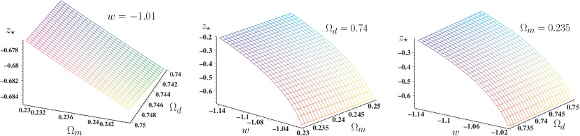
  Figure 1: Plot of the redshift $z_{\star}$ at which the total energy density of the brane reaches its minimum value.

  On the other hand, the two expanding branches are described by

  $$\bar{H}_{2}=\frac{1}{3}\left[2\sqrt{1-3b}\cos\left(\frac{\pi+\theta}{3}\right)+1\right],$$ (22)

  $$\bar{H}_{3}=\frac{1}{3}\left[2\sqrt{1-3b}\cos\left(\frac{\pi-\theta}{3}\right)+1\right],$$ (23)

  For $\theta\rightarrow 0$ the energy density $\bar{\rho}$ approaches $\bar{\rho}_{1}$ and the low energy regime connects at the limiting regime with the solution (19) where both solutions coincide; It can be further shown that $\bar{H}_{2}\leq\bar{H}_{3}$. The more interesting solution for us is the brane expanding solution described by Eq. (22): This solution constitutes a generalization of the self-accelerating DGP solution with GB effects Brown:2005ug , but within our herein model.

III The brane escaping the big rip and plunging into a sudden singularity

The usual self-accelerating DGP-GB solution is known to have a sudden singularity in the past, when the brane is filled by standard matter Brown:2005ug . Herein, we consider instead the brane filled with CDM plus phantom energy, performing an analysis aiming at future cosmic time. Starting from the modified Friedmann equation (10), it can be shown that the first derivative of the Hubble rate is

$$\dot{H}=\frac{\kappa_{4}^{2}\dot{\rho}}{3[2H-\frac{1}{r_{c}}(1+8\alpha H^{2})]},$$ (24)

where $\dot{\rho}$ is given by the equation of the energy conservation

$$\dot{\rho}+3H[\rho_{m}+(1+w)\rho_{d}]=0,$$ (25)

for the total energy density of the brane. Therefore, $\rho$ decreases initially until the redshift reaches the value $z_{\star}$,

$$z_{\star}=-1+\left[-(1+w)\frac{\Omega_{d}}{\Omega_{m}}\right]^{-\frac{1}{3w}},$$ (26)

where $\dot{\rho}=0$. Afterwards, the phantom matter starts dominating the expansion of the brane; indeed the brane starts super-accelerating ($0<\dot{H}$) and the total energy density of the brane starts growing as the brane expands. In figure 1, we plot the redshift $z_{\star}$ versus the observational values of the parameters $\Omega_{d}$, $\Omega_{m}$ and $w$. As can be noticed in this figure, the total energy density of the brane would start increasing only in the future. Furthermore, the larger is $|w|$, the sooner the phantom matter would dominate the expansion of the brane. $\Omega_{m}$ has the opposite effect while $\Omega_{d}$ has a much milder effect on $z_{\star}$.

Substituting Eq. (25) into Eq. (24), the first derivative of the Hubble rate reads,

$$\dot{H}=-\frac{\kappa_{4}^{2}H[(1+w)\rho_{d}+\rho_{m}]}{2H-\frac{1}{r_{c}}(1+8\alpha H^{2})}.$$ (27)

This equation shows that when the Hubble rate approaches the constant value,

$$H=\frac{r_{c}}{8\alpha}(\sqrt{1-3b}+1),$$ (28)

the first derivative of the Hubble parameter, $\dot{H}$, diverges, while the energy density of the brane remains finite. Thus, instead of a scenario where the energy density on the brane blueshifts and eventually diverges, with a big rip singularity emerging, we find that $(i)$ a finite value of the (dimensionless) energy density $\bar{\rho}=\bar{\rho}_{1}$ (the same applies for the pressure), and $(ii)$ a finite value for the (dimensionless) Hubble parameter $\bar{H}=\bar{H}_{2}$. Those values are reached in the limiting regime described by Eq. (19). And (iii) the first derivative of the Hubble parameter diverges at that point. Therefore, the energy density is bounded, i.e. the limit $z\rightarrow-1$ or $a\rightarrow\infty$ cannot be reached, and instead of a big rip singularity we get a sudden singularity, despite the brane being filled with phantom matter.

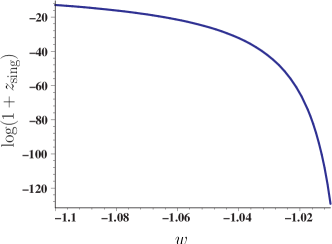
Figure 2: Values for the redshift at the sudden singularity, $z_{\textrm{sing}}$, for fixed value of $\Omega_{d}=0.75$, $\Omega_{m}=0.24$ and $\Omega_{r_{c}}=5.95\times 10^{-6}$ with respect to the parameter $w$.

The results above can be further elaborated, by establishing when the sudden singularity will happen (i.e., at which redshift and cosmic time values):

• In order to obtain the redshift $z_{\textrm{sing}}$ where the sudden singularity takes place, we equate the dimensionless total energy density of the brane (8) to its values at the sudden singularity (cf. Eq. (14)). The allowed values for $z_{\textrm{sing}}$ are plotted in Fig. 2 for the various values of the equation of state parameter $w$.

• Finally, using the relation between the scale factor and the redshift parameter, $a(t)=1/(1+z)$, one can write the Hubble rate as a function of the redshift parameter and its cosmic time derivative as follows

  $$H=\frac{\dot{a}}{a}=-\frac{\dot{z}}{1+z},$$ (29)

  and then integrating this equation, the cosmic time remaining before the brane hits the sudden singularity reads

  $$(t_{\textrm{sing}}-t_{0})H_{0}=-\int_{z=0}^{z=z_{\textrm{sing}}}\frac{dz}{(1+z)E(z)}.$$ (30)

  In the previous equation $t_{0}$ and $t_{\textrm{sing}}$ indicate the present time and the time at the sudden singularity, respectively. We can plot $t_{\textrm{sing}}$ for fixed values of $(\Omega_{m},\Omega_{d},\Omega_{\alpha})$; See Fig. 3. As we can notice from Fig. 3, the closer is the equation of state of the phantom matter to that of a cosmological constant, the farther would be the sudden singularity. The same plot is quite enlightening as we can compare the age of the universe, essentially $H_{0}^{-1}$, to the time left for such a sudden singularity to take place on the future of the brane. As we can see, such a sudden singularity would take place roughly in about 0.1 Gyr.

It is of interest to compare this estimate with the time at which a big rip would take place in a standard four-dimensional universe filled with phantom matter whose equation of state is constant. In ref. O2 , the time remaining for such a big rip singularity was estimated to be about 22 Gyr. However, notice that in O2 , $w=-1.5$ and $\Omega_{m}=0.3$ was used, whereas we have $w\in[-1.1,-1.01]$, $\Omega_{m}=0.24$; Our setting is also different. Within the framework of O2 , for $w=-1.1$ and $\Omega_{m}=0.24$, one retrieves a time of about 80 Gyr. In comparison, for the model presented in this paper, with $w=-1.5$ and $\Omega_{m}=0.3$, $\Omega_{d}=0.68$, $\Omega_{\alpha}=0.005$, the singularity emerges in $0.2$ Gyr. On the whole, although the universe would meet a “less severe” singularity in the future, this would happen much sooner that for the big rip case. In O2 , there are a few predictions concerning possible astronomical events that would indicate the emergence of the singularity herein exposed. Within our model, some of those events or other of similar impact could occur rather earlier.

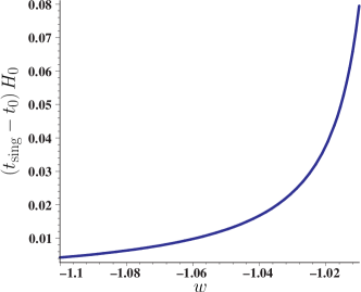
Figure 3: Variation of the cosmic time left before the brane hits the sudden singularity, $(t_{\rm{sing}}-t_{0})H_{0}$ (in dimensionless units), for fixed values of $\Omega_{d}=0.75$, $\Omega_{m}=0.24$ and $\Omega_{r_{c}}=5.95\times 10^{-6}$ with respect to the equation of state parameter $w$.

IV Conclusions and Outlook

The study of singularities occurring in the future is a subject of interest and several proposals for their removal or substitution have been advanced BouhmadiLopez:2004me ; Elizalde:2004mq ; Sergei6 ; Dabrowski:2006dd ; Kamenshchik:2007zj ; BouhmadiLopez:2009pu ; Sami:2006wj ; scalarfield . In this paper, we have considered a specific case and investigated whether a composition of specific IR and UV effects could alter a big rip singularity setting. More concretely, we employed a simple model: a DGP brane model, with phantom matter and a GB term for the bulk. The DGP brane configuration has relevant IR effects, whereas the GB component is important for high energies; phantom matter in a standard FLRW model is known to induce the emergence of big rip singularities Caldwell:2003vq .

Our analysis indicates that the big rip can be replaced by a sudden future singularity, through some intertwining between late-time dynamics and high energy effects. Subsequently, we determine values of the redshift and cosmic time, before the brane reaches the sudden singularity. These results can be contrasted with those, e.g., in O2 for the big rip occurrence in a FLRW setting.

We are aware that the herein conclusions are based in a rather particular result, that was extracted from a specific model. Subsequent research work would assist in clarifying some remaining issues. For example, it would be interesting to further study if and how other singularities can be appeased or removed by means of the herein combined IR and UV effects. On the other hand, it might be interesting to consider a modified Hilbert-Einstein action on the brane, which in addition could alleviate the ghost problem present on the self-accelerating DGP model by self-accelerating the normal DGP branch BouhmadiLopez:2009db , and see if some of the dark energy singularities can be removed or at least appeased in this setup. We hope to report on these lines in a forthcoming publication.

References

- (1) S. Perlmutter et al., Astrophys. J. 517, 565 (1999) [arXiv:astro-ph/9812133]; A. G. Riess et al., Astron. J. 116, 1009 (1998) [arXiv:astro-ph/9805201]; M. Kowalski et al., Astrophys. J. 686, 749 (2008) [arXiv:0804.4142 [astro-ph]].
- (2) D. N. Spergel et al.,Astrophys. J. Suppl. 148, 175 (2003) [arXiv:astro-ph/0302209]; ibid. Astrophys. J. Suppl. 170, 377 (2007) [arXiv:astro-ph/0603449]; E. Komatsu et al. [WMAP Collaboration], Astrophys. J. Suppl. 180, 330 (2009) [arXiv:0803.0547 [astro-ph]].
- (3) S. Cole et al., Mon. Not. Roy. Astron. Soc. 362, 505 (2005) [arXiv:astro-ph/0501174].
- (4) M. Tegmark et al., Astrophys. J. 606, 702 (2004) [arXiv:astro-ph/0310725].
- (5) V. Sahni, Class. Quant. Grav. 19 (2002) 3435 [arXiv:astro-ph/0202076].
- (6) R. R. Caldwell, Phys. Lett. B 545, 23 (2002) [arXiv:astro-ph/9908168].
- (7) L. Fernández-Jambrina and R. Lazkoz, Phys. Rev. D 70 (2004) 121503 [arXiv:gr-qc/0410124].
- (8) S. Nojiri, S. D. Odintsov and S. Tsujikawa, Phys. Rev. D 71 (2005) 063004 [arXiv:hep-th/0501025]; S. Nojiri and S. D. Odintsov, Phys. Rev. D 78 (2008) 046006 [arXiv:0804.3519 [hep-th]]; K. Bamba, S. Nojiri and S. D. Odintsov, JCAP 0810, 045 (2008) [arXiv:0807.2575 [hep-th]].
- (9) A. A. Starobinsky, Grav. Cosmol. 6 (2000) 157 [arXiv:astro-ph/9912054];
- (10) R. R. Caldwell, M. Kamionkowski and N. N. Weinberg, Phys. Rev. Lett. 91, 071301 (2003) [arXiv:astro-ph/0302506];
- (11) J. D. Barrow, Class. Quant. Grav. 21, L79 (2004) [arXiv:gr-qc/0403084].
- (12) S. Nojiri and S. D. Odintsov, Phys. Lett. B 595 (2004) 1 [arXiv:hep-th/0405078].
- (13) Y. Shtanov and V. Sahni, Class. Quant. Grav. 19 (2002) L101 [arXiv:gr-qc/0204040]; S. Nojiri and S. D. Odintsov, Phys. Rev. D 70 (2004) 103522 [arXiv:hep-th/0408170]; S. Nojiri and S. D. Odintsov, Phys. Rev. D 72 (2005) 023003 [arXiv:hep-th/0505215]; L. P. Chimento and R. Lazkoz, Class. Quant. Grav. 23 (2006) 3195 [arXiv:astro-ph/0505254]; M. Bouhmadi-López, P. F. González-Díaz and P. Martín-Moruno, Phys. Lett. B 659, 1 (2008) [arXiv:gr-qc/0612135]; M. Bouhmadi-López, P. F. González-Díaz and P. Martín-Moruno, Int. J. Mod. Phys. D 17, 2269 (2008) [arXiv:0707.2390 [gr-qc]].
- (14) M. Bouhmadi-López and J. A. Jiménez Madrid, JCAP 0505 (2005) 005 [arXiv:astro-ph/0404540].
- (15) E. Elizalde, S. Nojiri and S. D. Odintsov, Phys. Rev. D 70 (2004) 043539 [arXiv:hep-th/0405034].
- (16) M. C. B. Abdalla, S. Nojiri and S. D. Odintsov, Class. Quant. Grav. 22 (2005) L35 [arXiv:hep-th/0409177].
- (17) M. P. Da̧browski, C. Kiefer and B. Sandhöfer, Phys. Rev. D 74 (2006) 044022 [arXiv:hep-th/0605229].
- (18) A. Kamenshchik, C. Kiefer and B. Sandhöfer, Phys. Rev. D 76 (2007) 064032 [arXiv:0705.1688 [gr-qc]].
- (19) M. Bouhmadi-López, C. Kiefer, B. Sandhöfer and P. V. Moniz, Phys. Rev. D 79 (2009) 124035 [arXiv:0905.2421 [gr-qc]].
- (20) M. Sami, P. Singh and S. Tsujikawa, Phys. Rev. D 74 (2006) 043514 [arXiv:gr-qc/0605113].
- (21) M. Bouhmadi-López, Nucl. Phys. B 797 (2008) 78 [arXiv:astro-ph/0512124]; M. Bouhmadi-López and A. Ferrera, JCAP 0810 (2008) 011 [arXiv:0807.4678 [hep-th]]; M. R. Setare and E. N. Saridakis, JCAP 0903 (2009) 002 [arXiv:0811.4253 [hep-th]].
- (22) G. R. Dvali, G. Gabadadze, and M. Porrati, Phys. Lett. B 485, 208 (2000) [arXiv:gr-qc/0612135].
- (23) C. Deffayet, Phys. Lett. B 502 (2001) 199 [arXiv:hep-th/0010186].
- (24) K. Atazadeh and H. R. Sepangi, Phys. Lett. B 643, 76 (2006) [arXiv:gr-qc/0610107]; K. Atazadeh and H. R. Sepangi, JCAP 0901, 006 (2009) [arXiv:0811.3823 [gr-qc]]; K. Atazadeh and H. R. Sepangi, JCAP 0709, 020 (2007) [arXiv:0710.0214 [gr-qc]].
- (25) G. Kofinas, R. Maartens and E. Papantonopoulos, JHEP 0310 (2003) 066 [arXiv:hep-th/0307138]; R. A. Brown, R. Maartens, E. Papantonopoulos and V. Zamarias, JCAP 0511 (2005) 008 [arXiv:gr-qc/0508116].
- (26) R. G. Cai, H. S. Zhang and A. Wang, Commun. Theor. Phys. 44 (2005) 948 [arXiv:hep-th/0505186].
- (27) M. Bouhmadi-López and P. V. Moniz, Phys. Rev. D 78 (2008) 084019 [arXiv:0804.4484 [gr-qc]].
- (28) http://lambda.gsfc.nasa.gov/product/map/dr3/parameters.cfm.
- (29) R. Gregory, Prog. Theor. Phys. Suppl. 172 (2008) 71 [arXiv:0801.1603 [hep-th]].
- (30) See for example: S. M. Carroll, M. Hoffman and M. Trodden, Phys. Rev. D 68 (2003) 023509 [arXiv:astro-ph/0301273].
- (31) M. Abramowitz and I. Stegun, Handbook of Mathematical Functions (Dover, 1980).
- (32) R. Maartens and E. Majerotto, Phys. Rev. D 74, 023004 (2006) [arXiv:astro-ph/0603353]; R. Lazkoz and E. Majerotto, JCAP 0707, 015 (2007) [arXiv:0704.2606 [astro-ph]].
- (33) M. Bouhmadi-López, JCAP 0911 (2009) 011 [arXiv:0905.1962 [hep-th]].