Coarse-graining microscopic strains in a harmonic, two-dimensional solid and its implications for elasticity: non-local susceptibilities and non-affine noise.

Abstract

In soft matter systems the local displacement field can be accessed directly by video microscopy enabling one to compute local strain fields and hence the elastic moduli in these systems using a coarse-graining procedure. Here, we study this process in detail for a simple triangular lattice of particles connected by harmonic springs in two-dimensions. Coarse-graining local strains obtained from particle configurations in a Monte Carlo simulation generates non-trivial, non-local strain correlations (susceptibilities), which may be understood within a generalized, Landau type elastic Hamiltonian containing up to quartic terms in strain gradients (K. Franzrahe et. al., Phys. Rev. E 78, 026106 (2008)). In order to demonstrate the versatility of the analysis of these correlations and to make our calculations directly relevant for experiments on colloidal solids, we systematically study in detail various parameters such as the choice of statistical ensemble, presence of external pressure and boundary conditions. Crucially, we show that special care needs to be taken for an accurate application of our results to actual experiments, where the analyzed area is embedded within a larger system, to which it is mechanically coupled. Apart from the smooth, affine strain fields, the coarse-graining procedure also gives rise to a noise field ($\chi$) made up of non-affine displacements. Several properties of $\chi$ may be rationalized for the harmonic solid using a simple ”cell model” calculation. Furthermore the scaling behavior of the probability distribution of the noise field ($\chi$) is studied. We find that for any inverse temperature $\beta$, spring constant $f$, density $\rho$ and coarse-graining length $\Lambda$ the probability distribution can be obtained from a master curve of the scaling variable ${\mathcal{X}}=\chi\beta f/\rho\Lambda^{2}$.

I Introduction

Soft matter with its structural and elastic properties offers an attractive route to the design of new materials. In particular colloidal dispersions attract a lot of interest in this context. Surface chemistry or alterations in the composition of the solvent give an excellent control over the effective interactions in colloidal dispersions YETHI . By definition colloids lie in the range of the visible spectrum. Video microscopy HABD is therefore a straightforward means to gain information of the microscopic trajectories of the components of the system under study. Thus microscopic, thermal (or Brownian) fluctuations can be resolved directly in real space, making colloidal dispersions excellent model systems for the study of fundamental questions of the statistical physics of soft condensed matter. Two dimensional colloidal dispersions, for example, have been used successfully in studies on melting in two dimensions during the last decades STRAND ; SEN_KTHNY ; BIND_KTHNY ; GRUENB_MELT . In this paper we focus on the mechanical properties of such systems and consider, in detail, how they may be obtained from the microscopic particle trajectories.

Within linear elasticity, a solid in two-dimensions is described by eight unknown variables: the three stresses $\sigma_{ij}$, three strains $\epsilon_{ij}$ and two components of the displacement field $u_{i}$. Appropriately, there are also eight equations, namely the two equilibrium conditions $\partial\sigma_{ji}/{\partial x_{j}}+f_{i}=0$ (with $f_{i}$, the forces per unit volume within the body), three geometrical equations $\epsilon_{ij}=\left(\partial u_{i}/\partial x_{j}+\partial u_{j}/\partial x_{i}\right)/2$, and three constitutive equations $\sigma_{ij}=C_{ijkl}\epsilon_{kl}$. This set of equations may be solved for a given boundary condition in order to extract either the stresses or strains, given the elastic moduli, or the elastic moduli themselves, if the strains are known for a given stress configuration or vice versa. This manner of obtaining elastic moduli requires us to perturb the system using some external means e.g. laser tweezers WILLE . In contrast to this approach, one may calculate the tensor of elastic constants $C_{ijkl}$ of a system from fluctuations of the microscopic strains obtained by a coarse-graining procedure. Computing $C_{ijkl}$ in this way requires no external forces to be applied which may tend to change the very properties that are being measured SEN_FLUCM ; ZAHN ; MARAG . Recently, this procedure was further extended in Ref.KFRANZ2 to obtain even the non-local elastic susceptibilities.

The purpose of the present paper is twofold. Firstly, we present in great detail the analytic background of the coarse-graining procedure for obtaining elastic moduli and non-local susceptibilities (or strain-strain correlation functions) used in our earlier work KFRANZ2 . In order to demonstrate the versatility inherent to the analysis of these non-local elastic susceptibilities, we present systematic studies of a simple two dimensional lattice of particles connected by harmonic springs in the current paper. A comparison of the non-local susceptibilities in different statistical ensembles for various boundary conditions, system sizes and under different external conditions is given. Furthermore relations between the non-local susceptibilities and the elastic constants in systems surrounded by an embedding medium are derived. The proper interpretation of the correlation functions in such settings is discussed and visualized by use of the static susceptibility sum rule. Thus our aim in the present paper is to demonstrate various approaches in the analysis of the non-local strain correlation functions and to show how the analysis has to be adapted to the actual experimental situation. This study will thus greatly facilitate adoption of such techniques for routine analysis of experimental data at least for soft systems, which are close to being harmonic.

Secondly, apart from the above stated intent to establish a precise procedure for obtaining mechanical properties from microscopic configuration data, we also aim, to study in some detail fundamental aspects of the coarse-graining procedure itself. For example, an immediate problem is the presence of particle configurations within the coarse-graining volume, which are not describable in terms of affine deformations of any reference lattice, e.g. incipient vacancy-interstitial pairs. This is true for all coarse-graining volumes larger than an unit cell. What is the effect of these configurations on elasticity and how do they influence mechanical behavior? Recently, there has been significant progress in the study of non-affineness in solid plasticity - especially in the context of rheological properties of amorphous materials and granular solids which show jamming behavior FALK_LA ; LEMAI ; MALON . Localized non-affine regions consisting of particles capable of large reorientations have been shown to be involved in relaxation processes in these systems. Is there an analog of such regions in an ideal, crystalline solid? A study of these fluctuations in ideal solids, as presented in section IV, may help us understand complex dynamics in solids better.

The organization of this paper, together with a short summary of our main results is as follows. In section II we derive an analytic form of the non-local elastic response function, or compliance $\chi_{ij}(\vec{r},\vec{r}^{\prime})$ ($i=x,y$), which is defined as the strain $\varepsilon_{ij}(\vec{r}^{\prime})$ produced at position $\vec{r}^{\prime}$ due to a stress $\sigma_{ij}(\vec{r})$ at $\vec{r}$. In order to do this, we consider a Landau expansion CHAIKI of the free energy in terms of the strains, keeping up to quartic terms in the gradients. Next in section III we present Monte Carlo computer simulations of a harmonic crystal. The calculation of the local strain field corresponds to a coarse-graining procedure and allows us to construct the strain-strain correlation function, $G_{ij}$ which is related to the response function via $\chi_{ij}=(k_{B}T)^{-1}G_{ij}$. For a homogeneous solid without external load (i.e. $\langle\varepsilon_{i}(\vec{r})\rangle=0$) the correlation functions are given by $G_{ij}(\vec{r}^{\prime})=V<\varepsilon_{i}(\vec{0})\,\varepsilon_{j}(\vec{r}^{\prime})>$. The $<...>$ denote a thermal average (and in addition one over the choice of origin) and $k_{B}T$ is the Boltzmann constant times the temperature. We compare our results, obtained for a variety of ensembles and boundary conditions to that of the Landau theory. A common feature in experimental systems is the presence of an embedding medium, surrounding the analyzed region of the sample. The effects of such an embedding medium on the strain correlations are discussed and visualized by use of a statistical sum rule. One of our significant results is that though the forms of the correlation functions and their limiting values as predicted by the Landau theory are reproduced, the $G_{ij}$ obtained from simulations through our coarse-graining procedure differ by an additional background contribution which is not negligible. In section IV we argue that this is a consequence of non-affine displacements, which are not considered in the ansatz for the Landau theory. The amount of non-affinity in a given configuration can be quantified by calculating $\chi$, the deviation of the actual configuration from one obtained from an affine transformation of the reference lattice. We analyze this non-affineness in detail and show that the probability distribution of the non-affine field $P(\chi)$ can be computed within a simple “cell model” approximation. $P(\chi)$ shows well defined scaling properties with the spring stiffness $f$ and the coarse-graining length $\Lambda$. The auto-correlation function for $\chi$ is shown to be short ranged decaying rapidly for distances much larger than the coarse-graining length. Finally, we conclude our paper indicating future directions for research.

II Landau theory for the strains

The two dimensional elastic continuum described by the linear elastic Hamiltonian,

$$\beta{\cal H}_{0}=\frac{1}{2}\int d{\vec{r}}\,\,C_{ijkl}\epsilon_{ij}\epsilon_{kl}$$ (1)

is perpetually in a critical state CHAIKI . The displacement correlations $\langle{\vec{u}}({\vec{r}})\cdot{\vec{u}}({\vec{r}}\,^{\prime})\rangle$ decay algebraically and the solid shows quasi-long ranged order with the elastic susceptibilities diverging logarithmically with system size $L$. For all practical purposes, however, this weak divergence may be ignored and non-zero elastic moduli may be defined and computed. In real solids, an upper length scale cutoff is set by the typical distance between defect pairs.

The fact that the solid state is critical also implies that the Hamiltonian ${\cal H}_{0}$ in Eq.(1) is a fixed point Hamiltonian which should be invariant under a coarse- graining procedure, unless topological defects such as dislocations are present. This, again, is not strictly true, as we shall demonstrate in section III. This is because in a molecular system, any Hamiltonian such as ${\cal H}_{0}$ is realized only in an approximate, discretized sense, the displacements ${\vec{u}}$ being carried by the individual particles. Anticipating some of our results in section III, we use the following dimensionless Landau functional CHAIKI ; ERINGE :

$$\beta\mathcal{F} = \frac{1}{2}\int d^{2}x~{}\sum_{i=1}^{3}\left\{a_{i}e_{i}^{2}+c_{i}(\nabla e_{i})^{2}+c^{\prime}_{i}(\nabla^{2}e_{i})^{2}\right\}$$ (2)

Here with ($i=1-3$) the dimensionless constants $a_{i}$ are the elastic moduli of the system, while $c_{i}$ and $c^{\prime}_{i}$ are phenomenological coefficients and the three strains $e_{i}$ are given by: $e_{1}=\epsilon_{xx}+\epsilon_{yy}$, describing pure volume changes; $e_{2}=\epsilon_{xx}-\epsilon_{yy}$, describing deviatoric shear strains and $e_{3}=\frac{1}{2}(\epsilon_{xy}+\epsilon_{yx})$, describing pure shear strains. The phenomenological coefficients $c_{i}$ have the dimension of a $\textrm{length}^{2}$. Thus we interpret $\xi_{el,i}\sim\sqrt{c_{i}}$ as a correlation length. Note that unless noted otherwise throughout the paper all lengths are given in units of $a$, the lattice parameter of the underlying triangular lattice in the simulated systems.

The terms quadratic in the strains $e_{i}$ represent the local part in this ansatz. Non-local contributions are included via the gradient terms. Note that the Landau functional Eq.(2) should be strictly valid for excitations of wavelengths longer than a short-wavelength cutoff. Short wavelength excitations are suppressed by the gradient terms CHAIKI ; ERINGE and we have ignored the possibility of defects.

For non-uniform strains, spatial fluctuations of the strains couple and only one of the strain variables $e_{i}$ in this ansatz is an independent variable as we show below. Firstly, all forces within and on the system must cancel for the system to be in thermodynamic equilibrium, i.e. $\frac{\partial\sigma_{ij}}{\partial x_{j}}=0$ for a solid under zero external stress; the case of external hydrostatic stress is presented in section III.3. The stress tensor $\sigma_{ij}$ can be obtained directly from Eq.(2), as $\sigma_{ij}=\frac{\delta~{}\beta\mathcal{F}}{\delta\epsilon_{ij}}$ . For a two-dimensional crystal this condition reads in Fourier space:

$$k_{x}a_{1}\tilde{e}_{1}+k_{x}a_{2}\tilde{e}_{2}+k_{y}a_{3}\tilde{e}_{3}=0$$ (3)

$$k_{y}a_{1}\tilde{e}_{1}-k_{y}a_{2}\tilde{e}_{2}+k_{x}a_{3}\tilde{e}_{3}=0$$ (4)

In addition St Venant’s compatibility condition must be considered in the calculations, which ensures an unique relation between the displacement field $\vec{u}$ and the strain fields $\epsilon_{ij}$. For a two-dimensional crystal this simplifies to

$$-k^{2}\tilde{e}_{1}+(k_{x}^{2}-k_{y}^{2})\tilde{e}_{2}+4k_{x}k_{y}\tilde{e}_{3}=0$$ (5)

in Fourier space. With the help of these three conditions the kernels $\tilde{Q}_{ij}$ relating the strain variables $\tilde{e}_{i}=\tilde{Q}_{ij}\tilde{e}_{j}$ can be derived. The resulting relations are given in detail below:

$$\tilde{e}_{2} = -\left(\frac{4a_{1}+2a_{3}}{a_{1}+a_{2}}\right)\left(\frac{k_{x}k_{y}}{k_{x}^{2}-k_{y}^{2}}\right)\tilde{e}_{3}=\tilde{Q}_{23}\tilde{e}_{3}$$

$$\tilde{e}_{1} = -\left(\frac{2a_{3}-4a_{2}}{a_{1}+a_{2}}\right)\left(\frac{k_{x}k_{y}}{k^{2}}\right)\tilde{e}_{3}=\tilde{Q}_{13}\tilde{e}_{3}$$

$$\tilde{e}_{1} = \left(\frac{a_{3}-2a_{2}}{2a_{1}+a_{3}}\right)\left(\frac{k_{x}^{2}-k_{y}^{2}}{k^{2}}\right)\tilde{e}_{2}=\tilde{Q}_{12}\tilde{e}_{2}$$

Note that the properties of the correlation functions are set by the wave vector dependence of the kernels $\tilde{Q}_{ij}$.

We shall also need kernels relating the strains $e_{i}$ to the local, microscopic rotations given by the anti-symmetric part of the strain tensor $\theta=\left(\partial u_{y}/\partial x-\partial u_{x}/\partial y\right)/2$. Local rotations $\theta$ are related to the deviatoric strains $e_{2}$ and the pure shear strains $e_{3}$. These strains are coupled in case of the presence of a surrounding, embedding medium. Starting from the definitions of the strain variables the partial derivative $\partial^{3}\theta/\partial x^{2}\partial y$ can be expressed solely in terms of $e_{2}$, $e_{3}$ and $\theta$. Thus one obtains the following relation between the three shear strain variables in Fourier space:

$$\tilde{\theta}(k_{x}^{2}+k_{y}^{2})=(k_{x}^{2}-k_{y}^{2})\tilde{e}_{3}-k_{x}k_{y}\tilde{e}_{2}$$

We may now derive a new kernel relating $\tilde{\theta}$ to e.g. the pure shear strain $\tilde{e}_{3}$ using the previously derived kernel $\tilde{Q}_{23}$. This results in:

$$\tilde{e}_{3}=\frac{k_{x}^{4}-k_{y}^{4}}{(k_{x}^{2}-k_{y}^{2})^{2}+k_{x}^{2}k_{y}^{2}\left(\frac{4a_{1}+2a_{3}}{a_{1}+a_{2}}\right)}~{}\tilde{\theta}=\tilde{Q}_{3\theta}~{}\tilde{\theta}$$

As the considerations in section III.4 will show, it will be helpful to define the strain variable $e_{2\theta}=2\theta$ and analyze its two-point correlation function in embedded systems, such as the colloidal crystal discussed in KFRANZ2 .

Switching to a discretized notation, appropriate for comparison with our simulations, so that $e_{1}(\vec{x})\rightarrow e_{1,\vec{m}}$ and $\vec{x}\rightarrow\vec{R}_{\vec{m}}$, where $\vec{m}$ (a tuple of integer lattice indices) specifies the position on a coarse-graining, square mesh the free energy can be rewritten as,

$$\beta\mathcal{F} = \frac{v_{z}}{2}\sum_{\vec{m}}\sum_{i=1}^{3}\left(a_{i}e_{i,\vec{m}}^{2}+c_{i}(\nabla e_{i,\vec{m}})^{2}+c^{\prime}_{i}(\nabla^{2}e_{i,\vec{m}})^{2}\right)$$

Here $v_{z}=V_{z}/a^{2}$ is the dimensionless volume of the coarse-graining cell and the summation runs over all $N$ cells. One may use the above relations to finally express $\beta\mathcal{F}$ as a harmonic functional of only one of the strain components. This allows the direct calculation of the analytic form of the two-point correlation functions, as the partition function factorizes (e.g. GOLDF ). Here we choose as an example the strains $\tilde{e}_{1}$ and obtain the following expression for the functional, written as a sum over the wave vectors:

$$\beta\mathcal{F} = \frac{1}{2v}\sum_{\vec{k}}\{a_{1}+k^{2}c_{1}+k^{4}c^{\prime}_{1}+(a_{2}+c_{2}k^{2}+c^{\prime}_{2}k^{4})(\tilde{Q}_{21}(\vec{k}))^{2}+(a_{3}+c_{3}k^{2}+c^{\prime}_{3}k^{4})(\tilde{Q}_{31}(\vec{k}))^{2}\}\tilde{e}_{1,\vec{k}}\tilde{e}_{1,\vec{k}}^{*}$$

with $v=V/a^{2}$, the dimensionless volume of the system. It is now straight forward to calculate the two-point correlation function starting from its general definition and taking into account the fact, that the average strains $\langle e_{i}(\vec{r})\rangle$ in a crystal, which is under no load, is zero.

$$G_{ii}(\vec{r},\vec{r}^{\prime}) = \langle e_{i}(\vec{r})e_{i}(\vec{r}^{\prime})\rangle-\langle e_{i}(\vec{r})\rangle\langle e_{i}(\vec{r}^{\prime})\rangle$$

$$= \frac{1}{v^{2}}\sum_{\vec{k}\vec{k^{\prime}}}e^{i((\vec{k}\cdot\vec{r})(\vec{k}^{\prime}\cdot\vec{r}^{\prime}))}\langle\tilde{e}_{\vec{k}}\tilde{e}_{\vec{k}^{\prime}}\rangle$$

The calculation yields the following relation for the average of the Fourier coefficients:

$$\langle\tilde{e}_{\vec{k}}\tilde{e}_{\vec{k}^{\prime}}\rangle=\delta_{\vec{k}+\vec{k}^{\prime},\vec{0}}\langle|\tilde{e}_{\vec{k}}|^{2}\rangle=\delta_{\vec{k}+\vec{k}^{\prime},\vec{0}}v/A(\vec{k})$$

Where, $A(\vec{k})=a_{1}+k^{2}c_{1}+k^{4}c^{\prime}_{1}+(a_{2}+c_{2}k^{2}+c^{\prime}_{2}k^{4})(\tilde{Q}_{21}(\vec{k}))^{2}+(a_{3}+c_{3}k^{2}+c^{\prime}_{3}k^{4})(\tilde{Q}_{31}(\vec{k}))^{2}$. As $\tilde{G}_{ii}(\vec{k})=\langle|\tilde{e}_{\vec{k}}|^{2}\rangle/v$ one can now write down the analytic form of the strain-strain correlation functions or rather their inverse in detail. For $i=1,2,3$ the structure of the strain-strain correlation functions is the same, while for $i=2\theta$ it differs slightly:

$$\tilde{G}_{ii}(\vec{k}\neq 0)^{-1} = a_{i}+k^{2}c_{i}+k^{4}c^{\prime}_{i}$$

$$+\sum_{j\neq i,j=1}^{3}(a_{j}+c_{j}k^{2}+c^{\prime}_{j}k^{4})(\tilde{Q}_{j1}(\vec{k}))^{2}$$

$$\tilde{G}_{ii}(\vec{0})^{-1} = a_{i}$$

$$\tilde{G}_{2\theta 2\theta}(\vec{k}\neq 0)^{-1} = \Big{(}a_{3}+c_{3}k^{2}+c_{3}^{{}^{\prime}}k^{4}$$

$$+ \sum_{j=1}^{2}(a_{j}+c_{j}k^{2}+c_{j}^{{}^{\prime}}k^{4})(\tilde{Q}_{j3})^{2}\Big{)}(\tilde{Q}_{3~{}2\theta})^{2}$$

$$\tilde{G}_{2\theta 2\theta}(\vec{0})^{-1} = \frac{a_{3}}{4}$$

II.1 Properties of the strain-strain correlation functions

The analytic strain-strain correlation functions $\tilde{G}_{ii}(\vec{k})$ (the inverse of which were given in Eq.(6)) are plotted in figure 1. The set of parameters $a_{i}$, $c_{i}$ and $c^{\prime}_{i}$ used in figure 1 were obtained from Monte-Carlo simulations in the $NVT$ ensemble with periodic boundary conditions of a harmonic triangular lattice, to be discussed in section III.2. While the deviatoric and shear strain correlation functions $\tilde{G}_{22}$ and $\tilde{G}_{33}$ have four-fold symmetries, the correlation function of the dilatation $\tilde{G}_{11}$ has an eight-fold symmetry. The correlation functions may be interpreted as the response of the system to a localized perturbation at the origin. This perturbation is either a dilatation, a deviatoric shear or a pure shear. The deformation of the solid may be decomposed as a superposition of the eigenmodes of the system. The eigenmodes for a square box, are plane waves with polarizations either longitudinal or transverse to the coordinate axes with the eigenfrequencies forming a discrete spectrum: $\omega_{nm}=\frac{2\pi}{L}c_{\alpha}\sqrt{n^{2}+m^{2}}$ with $n,m\in N_{0}$. Thus the wave vector of the eigenmodes along the diagonal, i.e. ($n=m$), exhibits a four-fold degeneracy, while those parallel to the coordinate axis, i.e. $n\neq m$ and $n\neq m\neq 0$, have an eight-fold degeneracy. A local dilatation as perturbation results in a superposition of eigenmodes with four- as well as eight-fold degeneracy. This leads to the eight-fold rotational symmetry visible for the strain correlation function $\tilde{G}_{11}$. In contrast to this the two possible shear perturbations will excite elastic waves that are superpositions of exclusively eigenmodes with four-fold degeneracy. For this reason the corresponding correlation functions $\tilde{G}_{22}$ and $\tilde{G}_{33}$ exhibit only a four-fold rotational symmetry.

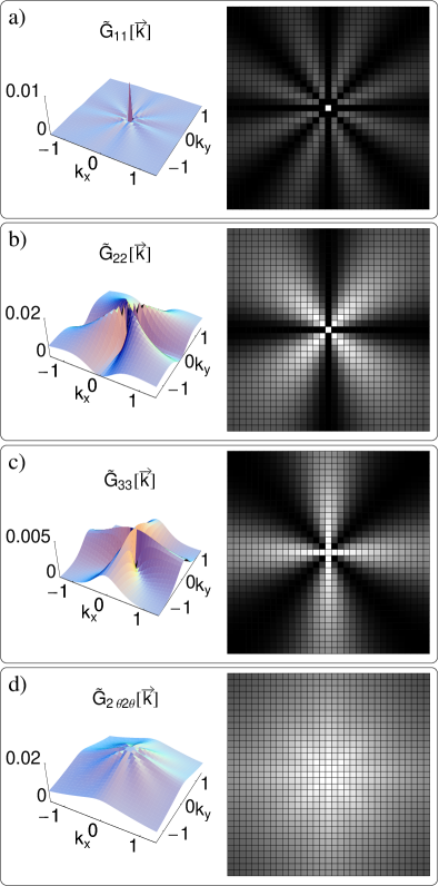
Figure 1: (Color online) The analytic form of the strain-strain correlation functions. For each function a surface plot and next to it a density plot are shown. In the density plot the maxima are white, minima are black. The set of parameters used for plotting was obtained from a Monte Carlo simulation of a harmonic triangular lattice in the $NVT$ ensemble with periodic boundary conditions: $a_{1}=97.4$, $a_{2}=48.1$, $a_{3}=198.2$, $c_{1}=54.3$, $c_{2}=37.4$, $c_{3}=118.2$, $c_{1}^{\prime}=-86.1$, $c_{2}^{\prime}=-1.3$ and $c_{3}^{\prime}=-18.8$. a) $G_{11}(\vec{k})$, b) $G_{22}(\vec{k})$ , c) $G_{33}(\vec{k})$ and d) $G_{2\theta 2\theta}(\vec{k})$.

As was discussed in KFRANZ3 , the presence of defects, breaks the rotational symmetries of the strain correlation functions.

The details of the structure of the correlation functions are dominated by the dependence of the kernels $\tilde{Q}_{ij}$ on the wave vector $\vec{k}$, especially the cases $k_{x}=k_{y}$, $k_{x}\rightarrow 0$ while $k_{y}\neq 0$ and $k_{y}\rightarrow 0$ while $k_{x}\neq 0$. In particular, we obtain the following relations:

$$\tilde{Q}_{12} = \left\{\begin{array}[]{cl}0&~{}~{}~{}~{}~{}\textrm{, for}~{}k_{x}=k_{y}\\ -\left(\frac{a_{3}-2a_{2}}{2a_{1}+a_{3}}\right)&~{}~{}~{}~{}~{}\textrm{, for}~{}k_{x}\rightarrow 0~{}~{}\textrm{,}~{}~{}k_{y}\neq 0\\ \left(\frac{a_{3}-2a_{2}}{2a_{1}+a_{3}}\right)&~{}~{}~{}~{}~{}\textrm{, for}~{}k_{y}\rightarrow 0~{}~{}\textrm{,}~{}~{}k_{x}\neq 0\\ \end{array}\right.$$ (10)

$$\tilde{Q}_{13} = \left\{\begin{array}[]{cl}\left(\frac{2a_{2}-a_{3}}{a_{1}+a_{2}}\right)&~{}~{}\textrm{, for}~{}k_{x}=k_{y}\\ 0&~{}~{}\textrm{, for}~{}k_{x}\rightarrow 0~{}~{}\textrm{,}~{}~{}k_{y}\neq 0\\ 0&~{}~{}\textrm{, for}~{}k_{y}\rightarrow 0~{}~{}\textrm{,}~{}~{}k_{x}\neq 0\\ \end{array}\right.$$ (14)

$$\tilde{Q}_{23} = \left\{\begin{array}[]{cl}\infty&~{}~{}\textrm{, for}~{}k_{x}=k_{y}\\ 0&~{}~{}\textrm{, for}~{}k_{x}\rightarrow 0~{}~{}\textrm{,}~{}~{}k_{y}\neq 0\\ 0&~{}~{}\textrm{, for}~{}k_{y}\rightarrow 0~{}~{}\textrm{,}~{}~{}k_{x}\neq 0\\ \end{array}\right.$$ (18)

For the kernel $\tilde{Q}_{3~{}2\theta}$ relating $e_{3}$ to $e_{2\theta}$ the behavior along the specific directions in Fourier space for $\vec{k}\rightarrow\vec{0}$ can be extracted from the behavior of the correlation function $\tilde{G}_{33}(\vec{k})$ and $\tilde{G}_{22}(\vec{k})$. Along the coordinate axis the kernel relating $\tilde{e}_{3}$ to $\tilde{e}_{2\theta}$ becomes a constant.

$$\tilde{Q}_{3~{}2\theta} = \left\{\begin{array}[]{cl}-1/2&\textrm{for}~{}k_{x}\rightarrow 0~{}~{}\textrm{,}~{}~{}k_{y}\neq 0\\ ~{}~{}1/2&\textrm{for}~{}k_{y}\rightarrow 0~{}~{}\textrm{,}~{}~{}k_{x}\neq 0\\ \end{array}\right.$$ (21)

Thus the continuous behavior of the correlation function $\tilde{G}_{33}(\vec{k})$ for $\vec{k}\rightarrow 0$ along the coordinate axis carries over to the correlation function $\tilde{G}_{2\theta 2\theta}(\vec{k})$. The behavior along the diagonals $k_{x}=k_{y}$ can be extracted from the behavior of the product of the kernels $\tilde{Q}_{23}^{2}\tilde{Q}_{3~{}2\theta}^{2}$, which can be shown to equal $1$. Upon insertion of these relations into the equations for the inverse of the correlation functions their behavior for these limiting cases can be extracted:

$$\tilde{G}^{-1}_{11}(\vec{k}) = \left\{\begin{array}[]{cl}~{}~{}~{}~{}~{}~{}~{}~{}~{}\infty&~{}~{}~{}~{}~{}~{}~{}~{}~{}\textrm{,}~{}~{}k_{x}=k_{y}\neq 0\\ ~{}~{}~{}~{}~{}~{}~{}~{}~{}\infty&~{}~{}~{}~{}~{}~{}~{}~{}~{}\textrm{,}~{}~{}k_{x}\rightarrow 0~{}~{}\textrm{,}~{}~{}k_{y}\neq 0\\ ~{}~{}~{}~{}~{}~{}~{}~{}~{}\infty&~{}~{}~{}~{}~{}~{}~{}~{}~{}\textrm{,}~{}~{}k_{x}\rightarrow 0~{}~{}\textrm{,}~{}~{}k_{y}\neq 0\\ \end{array}\right.$$ (25)

$$\tilde{G}^{-1}_{22}(\vec{k}) = \left\{\begin{array}[]{cl}a_{2}+c_{2}k^{2}+c_{2}^{\prime}k^{4}&\textrm{,}~{}~{}k_{x}=k_{y}\neq 0\\ \infty&\textrm{,}~{}~{}k_{x}\rightarrow 0~{}~{}\textrm{,}~{}~{}k_{y}\neq 0\\ \infty&\textrm{,}~{}~{}k_{x}\rightarrow 0~{}~{}\textrm{,}~{}~{}k_{y}\neq 0\\ \end{array}\right.$$ (29)

$$\tilde{G}^{-1}_{33}(\vec{k}) = \left\{\begin{array}[]{cl}\infty&\textrm{,}~{}~{}k_{x}=k_{y}\neq 0\\ a_{3}+c_{3}k^{2}+c_{3}^{\prime}k^{4}&\textrm{,}~{}~{}k_{x}\rightarrow 0~{}~{}\textrm{,}~{}~{}k_{y}\neq 0\\ a_{3}+c_{3}k^{2}+c_{3}^{\prime}k^{4}&\textrm{,}~{}~{}k_{y}\rightarrow 0~{}~{}\textrm{,}~{}~{}k_{x}\neq 0\\ \end{array}\right.$$ (33)

$$\tilde{G}^{-1}_{2\theta 2\theta}(\vec{k}) = \left\{\begin{array}[]{cl}a_{2}+c_{2}k^{2}+c_{2}^{\prime}k^{4}&\textrm{,}~{}~{}k_{x}=k_{y}\neq 0\\ (a_{3}+c_{3}k^{2}+c_{3}^{\prime}k^{4})/4&\textrm{,}~{}~{}k_{x}\rightarrow 0~{}~{}\textrm{,}~{}~{}k_{y}\neq 0\\ (a_{3}+c_{3}k^{2}+c_{3}^{\prime}k^{4})/4&\textrm{,}~{}~{}k_{x}\rightarrow 0~{}~{}\textrm{,}~{}~{}k_{y}\neq 0\\ \end{array}\right.$$ (37)

These considerations show, that in certain directions in Fourier space the shear strain variables become independent from each other and are continuous for $\vec{k}\rightarrow\vec{0}$ . These are the directions, along which a fit will give direct access to the elastic constants and correlation lengths of the system.

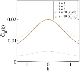
Figure 2: (Color online) Cuts of the analytic strain-strain correlation functions along specific directions in Fourier space. The set of parameters used for plotting is: $a_{1}=100$, $a_{2}=50$, $a_{3}=200$ and $c_{1}=54.3$, $c_{2}=37.4$, $c_{3}=118.2$, $c_{1}^{\prime}=-86.1$, $c_{2}^{\prime}=-1.3$, $c_{3}^{\prime}=-18.8$. The correlations lengths were obtained from a Monte Carlo simulation of a harmonic triangular lattice in the $NVT$ ensemble with periodic boundary conditions. $\tilde{G}_{11}(\vec{k})$ is shown along the direction $k_{y}=2k_{x}$, $\tilde{G}_{22}(\vec{k})$ along the diagonal $k_{x}=k_{y}$, $\tilde{G}_{33}(\vec{k})$ along the $k_{y}$-axis and $\tilde{G}_{2\theta 2\theta}(\vec{k})$ along the diagonal $k_{x}=k_{y}$ and along the $k_{y}$-axis.

Figure 2 shows cuts in Fourier space which correspond to these specific directions for the strain correlation functions $\tilde{G}_{ii}(\vec{k})$. For the correlation function of the pure shear strain $\tilde{G}_{22}(\vec{k})$ a cut along the diagonals is shown, while for the deviatoric strain correlation function $\tilde{G}_{33}(\vec{k})$ a cut along the coordinate axis is shown. The strain correlation function for the dilatation $\tilde{G}_{11}(\vec{k})$ in contrast is not continuous for $\vec{k}\rightarrow\vec{0}$. If one considers for example the direction $k_{y}=2k_{x}$ the kernels $\tilde{Q}_{ij}$ relating the strain variables turn into constant weighting factors: $\tilde{Q}_{21}=-\left(\frac{2a_{1}+a_{3}}{a_{3}-2a_{2}}\right)\left(\frac{5}{3}\right)$ and $\tilde{Q}_{31}=\left(\frac{a_{1}+a_{2}}{4a_{2}-2a_{3}}\right)\left(\frac{5}{2}\right)$. Thus along the direction $k_{y}=2k_{x}$ the inverse of the strain correlation function for the dilatation $\tilde{G}_{11}^{-1}(\vec{k})$ for $k\rightarrow 0$ is given by

$$\tilde{G}^{-1}_{11}(\vec{k}\rightarrow 0) = \Bigg{(}a_{1}+a_{2}\left[-\left(\frac{2a_{1}+a_{3}}{a_{3}-2a_{2}}\right)\left(\frac{5}{3}\right)\right]^{2}$$

$$~{}+a_{3}\left[\left(\frac{a_{1}+a_{2}}{4a_{2}-2a_{3}}\right)\left(\frac{5}{2}\right)\right]^{2}\Bigg{)}$$

$$\neq$$

$$\tilde{G}^{-1}_{11}(\vec{k}=0) = a_{1}$$

So the strain correlation function for the dilatation $\tilde{G}_{11}(\vec{k})$ exhibits a pronounced discontinuity for $\vec{k}\rightarrow\vec{0}$. In order to illustrate this fact, consider the set of parameters used in the simulations of a harmonic triangular lattice (to be discussed in section III). The choice of the spring constant sets the elastic constants of the system under consideration to $a_{1}=100$, $a_{2}=50$ and $a_{3}=200$. For $\vec{k}\rightarrow 0$ one has $\tilde{G}^{-1}_{11}(\vec{k}\rightarrow 0)\approx 3025$, which is approximately $30$ times as much as the value for $\vec{k}=0$, i.e. $\tilde{G}^{-1}_{11}(\vec{k}=0)=a_{1}=100$, set by the bulk modulus — showing that non-uniform dilations tend to be severely penalized in this solid.

Nevertheless, provided that the value of the bulk modulus is determined e.g. from $\tilde{G}_{11}(\vec{k}=\vec{0})$ the coefficients $c_{1}$ and $c_{1}^{\prime}$ can also be obtained by fitting one of the correlation functions along a cut in Fourier space. So in principle all $9$ parameters of the free energy functional can be determined from an analysis of the strain-strain correlation functions. Like the correlation function of the dilatation $\tilde{G}_{11}(\vec{k})$ the correlation function of the microscopic rotations shows an eight-fold rotational symmetry. Unlike $\tilde{G}_{11}(\vec{k})$, however, $\tilde{G}_{2\theta 2\theta}(\vec{k})$ is continuous for $\vec{k}\rightarrow\vec{0}$ along the coordinate axis and the diagonal (compare figure 2). Therefore fits along these directions can be used to determine the elastic constants $a_{2}$ and $a_{3}$ as well as the coefficients $c_{2}$, $c_{2}^{\prime}$ and $c_{3}$, $c_{3}^{\prime}$.

We shall next discuss the result of a coarse-graining procedure, which attempts to obtain these correlation functions and therefore the parameters of the Landau free energy functional from Monte Carlo simulations of the harmonic lattice. The coefficients of all the second and fourth order terms involving gradients of strain are found to be non-vanishing showing that coarse-graining generates these higher order non-local terms in the free energy.

III Monte Carlo simulations of a harmonic crystal

The analysis of a harmonic crystal is convenient for a comparison with the results of the Landau theory presented in the last section, since the elastic moduli can be directly calculated from the spring constants. We consider a harmonic triangular lattice with a Hamiltonian $\mathcal{H}=k_{B}T(f/2)\sum_{m,n=1}^{N}(|\vec{r}_{m}-\vec{r}_{n}|-a)^{2}$ where $f$ is the spring constant and $a$ the lattice parameter of the triangular lattice. The elastic moduli are related to the spring constant $f$ via: $K=a_{1}=(\sqrt{3}/2)f$, $\mu=a_{2}=(\sqrt{3}/4)f$ and $4\mu=a_{3}=\sqrt{3}f$. Furthermore the harmonic triangular lattice has been shown to be a successful model for the interpretation of experiments on colloidal crystals KEIM_HARMONIC . It is modeled by $N$ point-particles each of them hard-wired by spring constants $f$ to the six nearest neighbors. We have carried out Monte Carlo simulations in the constant $NpT$ and $NVT$ ensembles with periodic boundary conditions. We also mention briefly results for a system with open boundary conditions which were presented elsewhere KFRANZ2 . Next the influence of hydrostatic pressure is analyzed by Monte Carlo simulations in the constant $NpT$ ensembles with periodic boundary conditions. Finally we consider the effect of a surrounding elastic medium and finite size effects in order to make contact with experiments on colloids.

The knowledge of the configurations and the reference lattice allows for a direct calculation of the displacement field $\vec{u}(\vec{r})$. In order to calculate the corresponding strain field partial differentials of the displacement field have to be calculated. We follow the procedure by Falk and Langer FALK_LA and calculate the strain field by minimizing the error in the affine transformation that relates the actual configuration $\{\vec{r}\}$ to the reference lattice $\{\vec{R}\}$.

$$\vec{r}=\vec{R}+\vec{u}(\vec{R})=(\mathbf{1}+\mathbf{\epsilon})\vec{R}$$

The mean-squared error in this mapping $\chi$ is thus a measure of how well the given situation can be described within the framework of linear elasticity theory and quantifies the non-affinity of the given displacement field. Falk and Langer FALK_LA analyzed the temporal development of strains. Here we use an analogous definition for $\chi$ in thermodynamics equilibrium, evaluating the strains and non-affineness with respect to the reference lattice:

$$\chi(\vec{r}_{0})=\sum_{m=1}^{N_{B}}\sum_{i=1}^{2}\left(r_{m}^{i}-r_{0}^{i}-\sum_{j=1}^{2}(\delta_{ij}+\epsilon_{ij})[R_{m}^{j}-R_{0}^{j}]\right)^{2}$$

Here $\vec{r}_{0}$ is the position, at which the strains are to be calculated, and $N_{B}$ is the number of neighboring particles considered. This corresponds to a coarse-graining procedure, in which $N_{B}$ is set by the choice of coarse-graining length $\Lambda$, i.e. cutoff radius within which particles are considered in the calculation. For the results presented in this section, we have used a cutoff radius of $\Lambda=1.3$ resulting in $N_{B}=6$. In section IV we present some systematics showing how some of our results depend on the coarse-graining length $\Lambda$.

In the calculation of the strain-strain correlation functions a second coarse-graining step is employed, when mapping the triangular lattice to a square mesh. This facilitates the numerical Fourier transformation of the calculated real space correlation functions. The wave vectors are limited to the first Brillouin zone, i.e. $k_{j}\in[-\frac{\pi}{l_{m}},\frac{\pi}{l_{m}}]$, with $j=x,y$. Here $l_{m}$ represents the lattice parameter of the coarse-grained, square mesh. Care must be taken in the choice of $l_{m}$ to keep the coarse-graining volume large enough so that artifacts due to the discreteness of the triangular lattice (and insufficient averaging) are avoided. In most of the results presented here we used $l_{m}=2.25a$, where $a$ is the lattice parameter of the original, triangular lattice. Lastly, one also needs to be careful about correcting for global rotations and translations of the lattice especially for the case of open boundary conditions so as not to introduce artificial sources of error.

Simulations of the harmonic triangular lattice were done for three system sizes $N=3120$, $4736$ and $5822$. We first discuss the results for simulations with spring constant $\beta a^{2}f=200/\sqrt{3}$ in the $NpT$ ensemble with periodic boundary conditions (and external pressure $p=0$) and the $NVT$ ensemble with periodic boundary conditions. A crystal with open boundary conditions was discussed in detail in KFRANZ2 and will only be mentioned briefly. In what follows we analyze the influence of a hydrostatic, external pressure and of a surrounding, embedding medium.

III.1 $NpT$ ensemble with periodic boundary conditions

	$a_{1}$	$a_{2}$	$a_{3}$
calculated from $f$	$100~{}/\beta a^{2}$	$50~{}/\beta a^{2}$	$200~{}/\beta a^{2}$
from fluctuations
of $\mathbf{h}$	$98.9~{}/\beta a^{2}$	$49.4~{}/\beta a^{2}$	$196.7~{}/\beta a^{2}$
from $\tilde{G}(\vec{k}=\vec{0})$	$96.8~{}/\beta a^{2}$	$48.6~{}/\beta a^{2}$	$190.8~{}/\beta a^{2}$
from fits of $\tilde{G}(\vec{k}\neq\vec{0})$	-	$49.1~{}/\beta a^{2}$	$195.7~{}/\beta a^{2}$

Table 1: A comparison of the elastic constants as calculated from the spring constant $f$ and as obtained by use of various methods from data of a Monte Carlo simulation of a harmonic triangular lattice with $N=3120$ particles in the $NpT$ ensemble at zero hydrostatic pressure $\beta a^{2}p=0.0$ and spring constant $\beta a^{2}f=200/\sqrt{3}$.

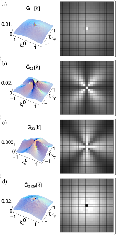
Figure 3: (Color online) Strain-strain correlation functions of a harmonic triangular lattice at zero hydrostatic pressure as obtained from Monte Carlo simulations in the $NpT$ ensemble with periodic boundary conditions. Results for a system with $N=3120$ particles and a spring constant $\beta a^{2}f=200/\sqrt{3}$ are shown. For each function a surface plot and next to it a density plot are displayed. In the density plot the maxima are white, minima are black.

For the simulations of the harmonic crystal in the $NpT$ ensemble we use the algorithm of Parinello and Rahman PARR_FLUCM . Here the information on the actual shape of the simulation volume, which is free to fluctuate in this ensemble, is saved in the transformation matrix $\mathbf{h}$. One of the advantages of this implementation is, that from the fluctuations of the transformation matrix $\mathbf{h}$ the fluctuations of the strain tensor can be calculated directly. The strain tensor is related to the transformation matrix via PARR_FLUCM :

$$\mathbf{\epsilon}=\frac{1}{2}\left(\mathbf{h}_{0}^{T,-1}\mathbf{G}\mathbf{h}_{0}^{-1}-\mathbf{1}\right)$$

where $\mathbf{h}_{0}$ is the transformation matrix of the reference lattice and $\mathbf{G}=\mathbf{h}^{T}\mathbf{h}$ contains the information of the actual shape of the simulation volume. Table 1 shows a comparison of the elastic moduli for the harmonic, triangular lattice as they are expected for the chosen spring constant $f$ and the values as they are obtained from the simulations in the $NpT$ ensemble by analyzing the fluctuations of the simulation volume.

Figure 3 shows the strain-strain correlation functions in Fourier space as they are obtained from the simulations in the $NpT$ ensemble with periodic boundary conditions. The eight-fold rotational symmetry in $\tilde{G}_{11}(\vec{k})$ is not resolved. The shear strain correlation functions show clearly a four-fold rotational symmetry, as was expected from the analytic predictions.

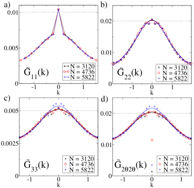
Figure 4: (Color online) Cuts of the strain-strain correlation functions in the $NpT$ ensemble with periodic boundary conditions at zero hydrostatic pressure along specific directions in Fourier space. a) $\tilde{G}_{11}(\vec{k})$ along $k_{y}=2k_{x}$, b) $\tilde{G}_{22}(\vec{k})$ along $k_{x}=k_{y}$, c) $\tilde{G}_{33}(\vec{k})$ and d) $\tilde{G}_{2\theta 2\theta}(\vec{k})$ along the $k_{y}$-axis. For a comparison the results for different system sizes are displayed. The horizontal broken lines mark the value expected from theory for the correlation functions at $\vec{k}=\vec{0}$.

Cuts along various directions in Fourier space of these functions are plotted in figure 4 for the three system sizes. As these cuts in Fourier space show, there is no systematic dependence on the system size in the correlation functions.

The discontinuities in the correlation functions are visible in figure 3 and 4. Nevertheless the extreme discontinuity one expects to observe in $\tilde{G}_{11}(\vec{k})$ from the analytic predictions is reduced to a factor of approximately $1.5$ instead of $30$, as a comparison of the cuts in figure 2 and in figure 4 a) shows. This indicates that there might be excitations in the system that are not captured by the assumption of purely affine strains. Along the cuts, for which $\tilde{G}_{22}(\vec{k})$ and $\tilde{G}_{33}(\vec{k})$ are continuous for $\vec{k}\rightarrow\vec{0}$, fitting with a generalize Lorentzian profile yields the elastic constants and via the coefficients $c_{i}$ the elastic correlation lengths. For the system with $N=3120$ we obtain the shear modulus as it is given in table 1 and the coefficients $c_{2}=34.3$, $c_{2}^{\prime}=-0.6$, $c_{3}=114.1$ and $c_{3}^{\prime}=-17.6$. So the elastic correlation lengths $\xi_{el,i}\sim\sqrt{c_{i}}$ are approximately $6$ and $11$ lattice parameters respectively.

Figure 4 d) shows cuts along the coordinate axis of $\tilde{G}_{2\theta~{}2\theta}(\vec{k})$. In these simulations the system as a whole is not an embedded system and is not free to rotate. Thus we cannot obtain the elastic modulus directly from the value of $\tilde{G}_{2\theta~{}2\theta}$ at the origin. This situation is different in a solid, which is embedded in a larger volume, as will be discussed in section III.4.

III.2 $NVT$ ensemble with periodic boundary conditions

Below, we describe simulations in the $NVT$ ensemble with periodic boundary conditions at a reduced density of $\varrho^{*}=1.0$. Table 2 lists the elastic constants calculated with the fluctuation method given by Squire et. al. SQUIRE . These authors also give a formula for calculating the stress tensor. An evaluation of the data yields $\sigma_{xy}=\sigma_{yx}=0.0$ and from the trace of the stress tensor $\beta a^{2}p=-\frac{1}{2}(\sigma_{xx}+\sigma_{yy})\approx 0.1$. So we verify that the simulations represent a solid at approximately zero hydrostatic pressure.

	$a_{1}$	$a_{2}$	$a_{3}$
calculated from $f$	$100~{}/\beta a^{2}$	$50~{}/\beta a^{2}$	$200~{}/\beta a^{2}$
using Squire et al. SQUIRE	$97.4~{}/\beta a^{2}$	$48.3~{}/\beta a^{2}$	$194.8~{}/\beta a^{2}$
from fits of $\tilde{G}(\vec{k}\neq\vec{0})$	-	$48.1~{}/\beta a^{2}$	$198.2~{}/\beta a^{2}$

Table 2: A comparison of the elastic constants as calculated from the spring constant $f$ and as obtained by use of various methods from data of a Monte Carlo simulation of a harmonic triangular lattice in the $NVT$ ensemble with periodic boundary conditions with $N=3120$ particles and spring constant $\beta a^{2}f=200/\sqrt{3}$.

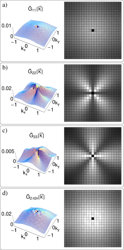
Figure 5: (Color online) Strain-strain correlation functions of a harmonic triangular lattice as obtained from Monte Carlo simulations in the $NVT$ ensemble with periodic boundary conditions. Results for s system with $N=3120$ particles and a $\beta a^{2}f=200/\sqrt{3}$ are shown. For each function a surface plot and next to it a density plot are displayed. In the density plot the maxima are white, minima are black.

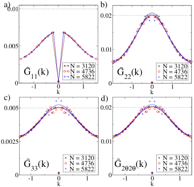
Figure 6: (Color online) Cuts of the strain-strain correlation functions in the $NVT$ ensemble with periodic boundary conditions along specific directions in Fourier space. a) $\tilde{G}_{11}(\vec{k})$ along $k_{y}=2k_{x}$, b) $\tilde{G}_{22}(\vec{k})$ along $k_{x}=k_{y}$, c) $\tilde{G}_{33}(\vec{k})$ and d) $\tilde{G}_{2\theta 2\theta}(\vec{k})$along the $k_{y}$-axis. For a comparison the results for different system sizes are displayed. The horizontal broken lines mark the value expected from theory for the correlation functions at $\vec{k}=\vec{0}$.

In this ensemble the $\vec{k}=\vec{0}$ values of the correlation functions cannot be used to calculate the elastic constants directly. We are simulating an undeformed state of the crystal, thus the integral over the fluctuations of the strains over the complete simulation volume tends to zero in this ensemble. Therefore only fits along the directions, for which the correlation functions are continuous for $\vec{k}\rightarrow\vec{0}$, give access to the elastic constants in this ensemble. As $\tilde{G}_{11}(\vec{k})$ has no such direction, the bulk modulus cannot be obtained in this way. From these considerations one expects the strain-strain correlation functions in the $NVT$ ensemble to differ from those in the $NpT$ ensemble for small absolute values of $\vec{k}$. Figure 5 shows surface plots and density plots of the strain-strain correlation functions in Fourier space. As in section III.1 the anisotropies are recovered well, except that the eightfold rotational symmetry of $\tilde{G}_{11}(\vec{k})$ is not resolved. The expected discontinuous jump to $\tilde{G}_{ii}(\vec{k}=\vec{0})=0$ ($i=1$, $2$, $3$) is clearly visible. Besides this, the correlation functions coincide with those obtained in the $NpT$ ensemble, as one can see by comparing figure 4 and 6, showing the same cuts in Fourier space for the various correlation functions. The elastic constants $a_{2}$ and $a_{3}$, as they are obtained from fitting the strain-strain correlation functions, are listed in table 2. They fall within $3-4\%$ of the theoretical values and have thus the same accuracy as the values obtained via Squire’s fluctuation formulae SQUIRE . In addition the elastic correlation lengths could be obtained from the coefficients: $c_{2}=37.4$, $c_{2}^{\prime}=-1.3$, $c_{3}=118.2$ and $c_{3}^{\prime}=18.8$. So consistent to the results obtained from the simulations in the $NpT$ ensemble $\xi_{el,i}\sim 6$ and $11$ lattice parameters respectively. Fitting e.g. $\tilde{G}_{22}(\vec{k}\neq\vec{0})$ along the direction $k_{y}=2k_{x}$ allows the determination of the coefficients $c_{1}=54.3$ and $c_{1}^{\prime}=-86.1$. Thus correlations of volume fluctuations decay over approximately 7 lattice parameters.

The harmonic, triangular lattice in the $NVT$ ensemble was also analyzed with open boundary conditions. The results were discussed in detail in KFRANZ2 .

III.3 The influence of hydrostatic pressure

How does an external, hydrostatic pressure - i.e. $\sigma_{xy}=\sigma_{yx}=0$ and $\sigma_{xx}=\sigma_{yy}=-p$ - influence the strain-strain correlation functions? Simulations of a harmonic, triangular lattice with spring constant $\beta a^{2}f=200/\sqrt{3}$ subjected to an external, hydrostatic pressure $\beta a^{2}p=20/\sqrt{3}$ show, that the shape of the correlation functions is not affected. The $NpT$ ensemble was chosen for this study. Strains were calculated with respect to the average lattice positions, that is the compressed lattice. The lattice parameter of this reference lattice $a^{\prime}=1.010465$ is smaller than the lattice parameter $a=(2/\sqrt{3})^{1/2}$ in the zero-pressure simulations. Therefore for a comparison with the theoretical values, which were given in units of $\beta a^{2}$, the $a_{i}$ as they are obtained e.g. from $\tilde{G}_{ii}(\vec{k}=\vec{0})$ must be rescaled to these units. Simulations were run for a system with $N=3120$ particles. For a direct comparison of the correlation functions in systems with and without a hydrostatic pressure cuts in Fourier space of the $\tilde{G}_{ii}(\vec{k})$ ($i=1,2,3,2\theta$) are shown in figure 7.

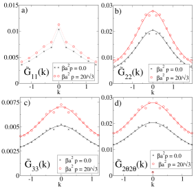
Figure 7: (Color online) Cuts of the strain-strain correlation functions in the $NpT$ ensemble with periodic boundary conditions along specific directions in Fourier space. Shown are the correlation functions obtained in a system without (crosses) external pressure and a system with $\beta a^{2}p=20/\sqrt{3}$ (circles). Both systems have $N=3120$ and a spring constant $\beta a^{2}f=200/\sqrt{3}$. a) $\tilde{G}_{11}(\vec{k})$ along $k_{y}=2k_{x}$, b) $\tilde{G}_{22}(\vec{k})$ along $k_{x}=k_{y}$, c) $\tilde{G}_{33}(\vec{k})$ and d) $\tilde{G}_{2\theta 2\theta}(\vec{k})$ along the $k_{y}$-axis.

calculated		$\mu=a_{2}+p$	$4\mu=a_{3}+4p$
from $f$	$100~{}/\beta a^{2}$	$=50~{}/\beta a^{2}$	$=200~{}/\beta a^{2}$
from
$\tilde{G}(\vec{k}=\vec{0})$	$88.8~{}/\beta a^{\prime 2}$	$a_{2}=36.0~{}/\beta a^{\prime 2}$	$a_{3}=137.6~{}/\beta a^{\prime 2}$
rescaled
values	$100.4~{}/\beta a^{2}$	$a_{2}=40.7~{}/\beta a^{2}$	$a_{3}=155.6~{}/\beta a^{2}$
		$\rightarrow\mu=52.2~{}/\beta a^{2}$	$\rightarrow 4\mu=201.8~{}/\beta a^{2}$

Table 3: The elastic moduli of the harmonic system calculated from the spring constant $\beta a^{2}f=200/\sqrt{3}$ in comparison to simulation results. Listed are the elastic constants $a_{i}$ as obtained from $\tilde{G}_{ii}(\vec{k}=\vec{0})$ for a simulation in the $NpT$ ensemble with periodic boundary conditions of a harmonic, triangular lattice with $\beta a^{2}p=20/\sqrt{3}$. For comparison with the theoretical values the $a_{i}$ obtained in units of the lattice parameter $a^{\prime}$ of the compressed reference lattice have to be rescaled to the lattice parameter $a$ of the zero-pressure reference lattice and the relation between the stiffness tensor $B_{ijkl}$ and the tensor of elastic constants $C_{ijkl}$ in a system with $\sigma_{ij}\neq 0$ need to be considered.

These show clearly the shift in the absolute values and the persistence of their shape. When relating the parameter $a_{i}$ to the elastic moduli of the system, one has to recall, that the strain-strain correlations are related to the stiffness tensor $B_{ijkl}$, which is defined via the stress-strain relations. These relate the variation of stress to the variation of strain, to first order in the strains, for the case, that an arbitrary initial configuration $\{\vec{R}\}$ is transformed to a final configuration $\{\vec{r}\}$ by an applied uniform stress. Thus $B_{ijkl}(\{\vec{R}\})\equiv\left(\partial\sigma_{ij}(\{\vec{r}\})/\partial\epsilon_{kl}\right)_{\{\vec{R}\}}=\frac{1}{2}\left(\sigma_{il}\delta_{jk}+\sigma_{jl}\delta_{ik}+\sigma_{ik}\delta_{jl}+\sigma_{jk}\delta_{il}-2\sigma_{ij}\delta_{kl}\right)+C_{ijkl}$ WALLA . The stiffness tensor explicitly depends on the applied stress. Only for the case that $\sigma_{ij}=0$ is it equivalent to the tensor of the elastic constants $C_{ijkl}$. For the calculation of the elastic moduli the following combinations are needed:

$$\frac{1}{2}\left(B_{xxxx}+B_{xxyy}\right) = \frac{1}{2}\left(C_{xxxx}+C_{xxyy}\right)-\frac{1}{2}\left(p-p\right)$$

$$= K$$

$$\frac{1}{2}\left(B_{xxxx}-B_{xxyy}\right) = \frac{1}{2}\left(C_{xxxx}-C_{xxyy}\right)-\frac{1}{2}\left(p+p\right)$$

$$= \mu-p$$

$$B_{xyxy} = C_{xyxy}-p=\mu-p$$

Thus the bulk modulus can be directly obtained from $a_{1}$, while from $\tilde{G}_{22}(\vec{k})$ one extracts $a_{2}=\mu-p$ and from $\tilde{G}_{33}(\vec{k})$ one obtains $a_{3}=4(\mu-p)$. The values of the elastic moduli calculated according to this scheme are given in table 3. They lie within $4.4\%$ of the theoretical values.

III.4 Effects of an embedding medium and finite-size

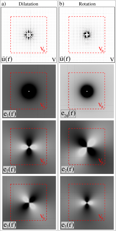
Figure 8: (Color online) A schematic drawing of the displacement field $\vec{u}(\vec{r})$ as it results from a given perturbation at the origin: a) a dilatation and b) a rotation a the disk at the origin. If the analyzed volume $V_{B}$ (broken red line) does not coincide with the volume of the complete system $V$ (black line), the energy needed for the displacements in the embedding medium ($V-V_{B}$) must be taken into account in the interpretation of the correlation functions.

Often the strain-strain correlations cannot be evaluated over the complete crystal. In experiments as for example a two dimensional colloidal crystal ZAHN ; KFRANZ2 configurational data is taken via video microscopy. Here the area accessible to the video camera is far smaller than the complete sample size. In these cases only a sub-system embedded in a larger continuum is analyzed. As Zahn et al. ZAHN noted the presence of an infinite, embedding medium alters the relation of the strain fluctuations to the elastic moduli.

The strain-strain correlation functions are the response functions to a strain perturbation at the origin. Figure 8 shows schematically the resulting displacement field and strain fields for the cases that this perturbation is a) a dilatation and b) a rotation. The connection between the strain correlations and the elastic moduli was derived under the assumption, that the considered functional of the free energy accounts for the free energy of the complete system (equipartition theorem). For the case that the volume $V_{B}$ over which the strain-strain correlation function are calculated is not equal to the complete system volume $V$ this assumption is not fulfilled any more. As can be seen in the schematic plots of the strain fields in figure 8 the energy related to the resulting strain field outside $V_{B}$ cannot be neglected for $V_{B}\neq V$.

Following the argument by Zahn et al. ZAHN , but considering a finite embedding continuum, we show that the influence of the surrounding medium on the strain fluctuations within the analyzed volume $V_{B}$ depends on the relative size of $V_{B}$ in comparison to the complete system volume $V$, i.e. the ratio of $V_{B}/V$. For the derivation of the formulae we consider first a homogeneous dilatation of a disk $V_{B}=\pi R_{B}^{2}$ in a surrounding medium of volume $V=\pi R^{2}$ and second a pure shear, which can be realized by a rotation by an angle $\theta$ of the disk with volume $V_{B}$. For these considerations we work in polar coordinates, where we have $e_{1}=(\epsilon_{rr}+\epsilon_{\varphi\varphi})$, $e_{2}=(\epsilon_{rr}-\epsilon_{\varphi\varphi})$ and $e_{3}=\epsilon_{r\varphi}$. In both cases considered here it is assumed that the displacement field on the boundary of the complete system is given by $\vec{u}(\vec{r}=\vec{R}_{boundary})=\vec{0}$.

III.4.1 Homogeneous dilatation

An isotropic expansion of a disk embedded in a finite medium is given by: $R_{B}\rightarrow R_{B}+\Delta r$. The resulting displacement field in polar coordinates is given by:

$$u_{\varphi}=0~{}~{}\textrm{,}~{}~{}~{}~{}u_{r}=\Bigg{\{}{\Delta r\frac{r}{R_{B}}\qquad\textrm{for}\qquad r<R_{B}\atop{\Delta r\frac{R_{B}}{r}\qquad\textrm{for}\qquad r>R_{B}}}$$

From this it is straight forward to calculate the resulting strain field and consequently the Free Energy density $f=\frac{1}{2}\left[K(\epsilon_{rr}+\epsilon_{\varphi\varphi})^{2}+\mu\left((\epsilon_{rr}-\epsilon_{\varphi\varphi})^{2}+4\epsilon_{r\varphi}^{2}\right)\right]$ of the system under load. Thus the total energy needed for such an expansion in a finite system of volume $V=\pi R^{2}$ is given by $E=\int_{0}^{2\pi}\int_{0}^{R}rd\varphi dr~{}f=\left(V_{B}/2\right)\left(\Delta V_{B}/V_{B}\right)^{2}\left[K+\mu\left(1-\left(V_{B}/V\right)\right)\right]$. For such a system equipartition tells us thus, that the strain fluctuations are no longer set by the bulk modulus of the system, but aquire in the embedded system a term dependent on the shear modulus and on the ratio $V_{B}/V$:

$$\frac{k_{B}T}{V_{B}}\langle e_{1}^{2}\rangle=\frac{1}{K+\mu\left(1-\left(\frac{V_{B}}{V}\right)\right)}$$

Therefore the strain-strain correlation function $G_{11}(\vec{r})$ no longer provides access to the bulk modulus, but to a $V_{B}/V$-dependent combination of bulk and shear modulus.

III.4.2 Pure shear

A rotation of the disk as a rigid body within the embedding medium by an infinitesimal angle $\Delta\varphi$ changes a given orientation $\varphi$ to $\varphi+\Delta\varphi$. The resulting displacement field is given by:

$$u_{r}=0~{}~{}\textrm{,}~{}~{}~{}~{}u_{\varphi}=\Bigg{\{}{0\qquad\qquad\quad\textrm{for}\qquad r<R_{B}\atop{\Delta\varphi\frac{R_{B}^{2}}{r}\qquad\quad\textrm{for}\qquad r>R_{B}}}$$

From the corresponding strain field the Free Energy density can be determined and integration over the complete system yields the energy required for such a rotation: $E=\mu(2\Delta\varphi)^{2}V_{B}\left(1-\left(V_{B}/V\right)\right)/2$. In case of infinitesimal rotation angles $\Delta\varphi$ this angle can be identified with the anti-symmetric part of the strain tensor $\theta=\left(\partial u_{y}/\partial x-\partial u_{x}/\partial y\right)/2$. Equipartition relates the fluctuations in $e_{2\theta}$ to the shear modulus $\mu$:

$$\frac{k_{B}T}{V_{B}}\langle e_{2\theta}^{2}\rangle=\frac{1}{\mu\left(1-\left(\frac{V_{B}}{V}\right)\right)}$$

This relation depends also on the ratio $V_{B}/V$, as the energy required for the rotation of a disk, which is not embedded in a surrounding medium, tends to zero. The analysis of the strain variable $2\theta$ offers thus an independent, direct route to the determination of the shear modulus in an embedded system.

These considerations show that in order to obtain accurate elastic moduli from the analysis of the strain fluctuations the relative size of the analyzed system to the complete, finite system should to be known. Nevertheless for the case of the colloidal crystal KFRANZ2 the situation is close to the limiting case of $\frac{V_{B}}{V}\rightarrow 0$. Here the influence of the surrounding medium on the analyzed system is dominant. The strain variables $e_{1}$ and $e_{2\theta}$ can be used to extract the elastic moduli. Thus the two-dimensional colloidal crystal, as discussed in detail in KFRANZ2 ; KFRANZ3 is an example for a completely embedded system. In contrast to this in simulations the complete system can be analyzed, which corresponds to the limiting case of $\frac{V_{B}}{V}\rightarrow 1$. For this case each of the strain-strain correlation functions of the strain variables $e_{1}$, $e_{2}$ and $e_{3}$ give directly access to the corresponding elastic moduli $a_{i}$. The effect of the embedding medium can be visualized by looking at a statistical sum rule, as will be discussed in the next paragraph.

III.4.3 Analysis of a statistical sum rule

The sum rule for the generalized susceptibility provides another way of extracting the elastic moduli from the strain-strain correlation functions. The coarse-grained system represents a homogeneous continuum and is thus translationally invariant. For such systems the susceptibilities are directly related to the correlation functions. In Fourier space this reads $\tilde{\chi}_{T}(\vec{k})=\beta\tilde{G}(\vec{k})$. From this the static susceptibility sum rule follows GOLDF :

$$\chi_{T}=\lim_{\vec{k}\to 0}\tilde{\chi}_{T}(\vec{k})=\beta\tilde{G}(\vec{k})|_{\vec{k}=\vec{0}}=\beta\int d\vec{r}~{}G(\vec{r})$$

Thus an integration of the correlation functions in real space yields directly the elements of the compliance tensor $S_{ijkl}$, which correspond to the generalized susceptibilities. The compliance tensor is the inverse of the stiffness tensor $B_{ijkl}$. In the case that no external stresses act on the system this is equivalent to the tensor of the elastic constants $C_{ijkl}$ WALLA . The $S_{ijkl}$ obtained from such an analysis depend on the integration volume $V_{B}$. Thus in order to obtain systems-size independent values an additional finite-size scaling analysis should be employed.

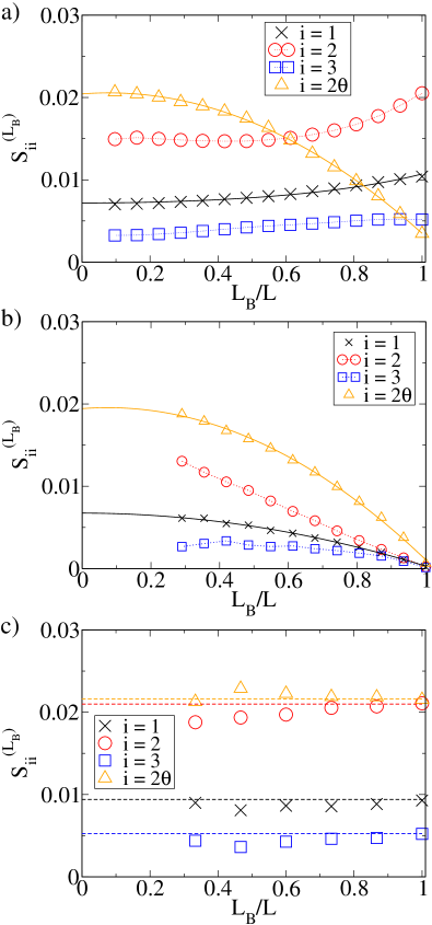
Figure 9: (Color online) Compliances $S_{ii}$ as they are obtained from the sum rule as a function of the ratio of analyzed volume $V_{B}=L_{B}^{2}$ to the complete simulation volume $V=L^{2}$. Shown are the results of Monte Carlo simulations of a harmonic triangular lattice with $N=5822$ particles and spring constant $\beta a^{2}f=200/\sqrt{3}$. Lines are a fit to the data with the formulae given in the text, while the dotted lines are a guide for the eyes. a) $NpT$ ensemble with periodic boundary conditions. b) $NVT$ ensemble with periodic boundary conditions. c) $NVT$ ensemble with open boundary conditions. Here dashed lines show the value for $L_{B}/L=1$ as a comparison.

Figure 9 shows the compliances $S_{ii}$ ($i=1$, $2$, $3$ and $2\theta$) as a function of the ratio of the integration volume $V_{B}$ to the complete simulation volume $V$, i.e. $V_{B}/V=L_{B}/L$, as they are obtained from the simulation data of the harmonic triangular crystal at zero external pressure in the $NpT$ and $NVT$ ensemble with different boundary conditions. A comparison shows directly how the choice of ensemble and the choice of boundary conditions influences the results. These are so called explicit and implicit finite-size effects ROMAN2 . In addition this analysis visualizes the effects of the embedding medium on the compliances $S_{ii}$. Figure 9 a) shows the results from simulations in the $NpT$ ensemble with periodic boundary conditions. The complete system contains $N=5822$ particles, that are connected via springs of spring constant $\beta a^{2}f=200/\sqrt{3}$. The strain-strain correlation functions are directly related to the elastic moduli in this ensemble, due to the fact that the volume itself fluctuates. Thus one can obtain the elastic moduli directly from the $S_{ii}$ at $L_{B}/L=1$. For the considered system we find: $S_{11}^{(L)}=0.01025$, $S_{22}^{(L)}=0.02050$, $S_{33}^{(L)}=0.00512$ and $S_{2\theta 2\theta}^{(L)}\rightarrow 0$, resulting in $a_{1}=97.5$, $a_{2}=48.7$ and $a_{3}=195.2$. These values lie within $2.5\%$ of the expected values. The accuracy of this approach compares to that of the methods for the calculation of the elastic moduli discussed before. From the considerations in III.4.1 one expects the following functional dependence of $S_{11}$ on $L_{B}/L$:

$$S^{(L_{B})}_{11} = V_{B}\langle e_{1}^{2}\rangle/(k_{B}T)=\left[K+\mu\left(1-\left(L_{B}^{2}/L^{2}\right)\right)\right]^{-1}$$

The black solid line in figure 9 a) is a fit with this equation to the data (crosses). From the fit parameters the following elastic moduli are extracted: $a_{1}=K=93.4$ and $\mu=a_{2}=45.8$. Figure 9 a) shows clearly the increasing impact the surrounding medium has on $S_{11}$ as $L_{B}/L$ diminishes. In the limit $V_{B}/V\rightarrow 0$ it yields the sum of the elastic moduli $K$ and $\mu$. It is apparent from figure 9 a), that as soon as $V_{B}/V<1$, the compliances $S_{22}$ and $S_{33}$ cannot be directly related to the shear modulus any more.

The considerations in III.4.2 suggest, that the compliance $S_{2\theta 2\theta}$ should diverge as $V_{B}/V\rightarrow 1$. This relates to the fact, that the energy needed for rotating an embedded disk goes to zero as the embedding material is removed. This divergence cannot be seen in the simulation data, as in simulations with periodic boundary condition the system as a whole cannot rotate. The fact, that there is no divergence of $S_{2\theta 2\theta}$ for $V_{B}/V\rightarrow 1$, is therefore an implicit finite-size effect. In order to extract the shear modulus from the compliance $S_{2\theta 2\theta}$ a polynomial in $(L_{B}/L)$ was fitted to the data (open triangles). From the limit $V_{B}/V\rightarrow 0$ the shear modulus is extracted: $\mu=48.9$.

In the $NVT$ ensemble with periodic boundary conditions the compliances as a function of $L_{B}/L$ exhibit a different dependence on $L_{B}/L$, as figure 9 b) shows. An unstrained state of the triangular lattice is analyzed in these simulations, therefore the integral of the correlation functions over the complete system goes to zero and gives no access to the elastic moduli. This is an explicite finite-size effect. Nevertheless from the limit $V_{B}/V\rightarrow 0$ one can extract the elastic moduli as in the case of the simulations in the $NpT$ ensemble with periodic boundary conditions from the compliances $S_{11}$ (crosses) and $S_{2\theta 2\theta}$ (open triangles). Fits with a polynomial in $(L_{B}/L)$ are plotted as solid lines in figure 9 b). From the case of maximum embedding one extracts $a_{1}+a_{2}=K+\mu=148.3$ from $S_{11}$ and $a_{2}=51.5$ from $S_{2\theta 2\theta}$ in figure 9 b). These values compare to the values obtained by different methods as they are given in table 2.

The compliances $S_{ii}^{L_{B}}$ shown in figure 9 c) are obtained from data of simulations in the $NVT$ ensemble with open boundary conditions as they were presented in KFRANZ2 . These show in contrast no systematic dependence on $V_{B}/V$. The maximum analyzed volume, which will for this case be denoted by $V=L^{2}$, is approximately one fourth of the complete system volume. Averaging over the positions of origin, as it is done in the calculation of the strain-strain correlation functions in the system with open boundaries, results in an averaging over sub-systems with partial to complete embedding. For this type of averaging the $\vec{k}=\vec{0}$ values of all considered strain-strain correlation functions give access to the elastic moduli of the system KFRANZ2 . The effect of this type of averaging shows up most prominently in the fact that $S_{2\theta 2\theta}$ does not tend to zero for $L_{B}/L\rightarrow 1$, but approaches the value of $S_{22}$. Extracting the elastic moduli from the compliances for $L_{B}/L=1$ in figure 9 c) yields $S^{(L)}_{11}=0.00940\rightarrow a_{1}=106.9$, $S^{(L)}_{22}=0.02100\rightarrow a_{2}=47.6$, $S^{(L)}_{33}=0.00525\rightarrow a_{3}=190.4$ and $S^{(L)}_{2\theta 2\theta}=0.02160\rightarrow a_{2}=46.4$. The accuracy of these values is the same as in KFRANZ2 . The deviation from the theoretical values is larger in this case, as the finite system with open boundary conditions is influenced in its elastic properties by the missing, stabilizing bonds for particles at the surfaces.

IV The statistics of non-affine fluctuations

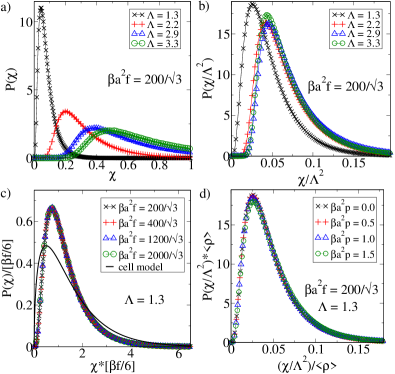
Figure 10: (Color online) Plots of the probability distribution of the non-affinity parameter $\chi$ from simulations in the $NpT$ ensemble with periodic boundary conditions and $N=3120$ particles. (a) Plot of the probability distribution of $P(\chi)$ vs $\chi$ for various coarse-graining length $\Lambda$. (b) The probability distribution of $\chi/\Lambda$ shows a data collapse for $\Lambda\geq 2.2$. (c) Data for various spring constants $f$ collapse onto each other. The prediction from a simple cell model (black line) is shown for comparison. (d) Data from simulations at various hydrostatic pressure $p$ scale with the resulting average density $\langle\varrho\rangle$.

The coarse-graining process described in section III projects the configurations generated by our microscopic Hamiltonian onto strain fields which are smooth over distances larger than the coarse-graining length $\Lambda$. It also generates a conjugate noise CHAIKI which represents those fluctuations which cannot be captured during coarse-graining. This is easily understood once it is realized that, coarse-graining retains only that part of the particle displacements $\vec{u}=\vec{r}-\vec{R}$ in a configuration which can be obtained from the reference lattice $\vec{R}$ by an affine transformation: $\vec{r}=(\mathbf{1}+\epsilon)\vec{R}$. An affine transformation constrains all parallel lines in the reference lattice to remain parallel, which is clearly impossible to satisfy for an arbitrary configuration coarse-grained over volumes larger than an unit cell. Indeed, the quantity $\chi$ as defined in Eq. (III) has the dimension of Length² and scales as $\Lambda^{2}$. This may be seen by comparing figure 10 (a) and (b). Figure 10 shows the probability distribution $P(\chi)$ and its scaling behavior for various choices of parameters. While 10 (a) shows a clear dependence of the amount of non-affinity on the coarse-graining length $\Lambda$, figure 10 (b) shows a collapse of the distributions for the scaled quantity $\chi/\Lambda^{2}$ for $\Lambda>2.2$. This corresponds to a minimum of $18$ neighbors to the central particle, that are taken into account in the calculation of the strain field via the minimization of $\chi$. These distributions show a constant offset from $\chi/\Lambda^{2}=0$. By contrast $\Lambda=1.3$ shows no such offset, meaning that for the calculation of the affine strain field only the minimal neighborhood, i.e. the $6$ nearest neighbors, allows for a global minimization of $\chi$. In addition the probability distributions of the non-affine parameter $\chi$ also scale with with the spring constant $f$ (figure 10 (c)) and in simulations run at various hydrostatic, external pressure $p$ with the resulting average density $\langle\varrho\rangle$ (figure 10 (d)). One can therefore obtain the probability distribution for $\chi$ for any inverse temperature $\beta$, spring constant $f$, density $\rho$ and coarse-graining length $\Lambda$ from a generalized extreme value probability distribution function. This master curve is $P({\mathcal{X}})=\left(\left(1+0.27\cdot z\right)^{(-1/0.27)-1}e^{-\left(1+0.27\cdot z\right)^{-1/0.27}}\right)/2.012$ with $z=\left({\mathcal{X}}-3.127\right)/2.012$, which we obtain from a fit to the simulation data, with the scaling variable ${\mathcal{X}}=\chi\beta f/\rho\Lambda^{2}$, independent of system size $N$ and the choice of ensemble.

We show below that features of $P(\chi)$, like the dependence on the spring constant $f$, may be rationalized within a simple “cell model” calculation. In this model each particle is assumed to fluctuate within the cage of its $6$ nearest neighbors which suffers, at most, an affine distortion (see figure 11). The only source of non-affinity comes from the displacement of the central particle from its equilibrium position.

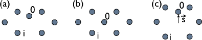
Figure 11: (Color online) Example configuration (a) consisting of a central particle $0$ and neighboring particles $i=1,6$ which can be decomposed into a purely affine deviatoric distortion (b) together with a non-affine displacement ${\vec{s}}$ of the central particle $0$ (c).

For such a subset of configurations, one may simply decompose each configuration $\{\vec{r}\}$ as that obtained by an affine transformation plus a non-affine displacement ${\vec{s}}$ of the central particle within an undistorted hexagonal cell. The non-affinity parameter $\chi$ may then be calculated to be,

$$\chi = \sum_{m=1}^{6}\sum_{i=1}^{2}\big{(}r_{m}^{i}-r_{0}^{i}-\sum_{j=1}^{2}(\delta_{ij}+\epsilon_{ij})[R_{m}^{j}-R_{0}^{j}]\big{)}^{2}$$

$$= \sum_{m=1}^{6}\sum_{i=1}^{2}\left(r^{i}_{m}-r^{i}_{0}-(R^{i}_{m}-R^{i}_{0})\right)^{2}=6s^{2}$$

Within this approximation the ensemble average contributes to the Lindemann parameter $l$, as $\langle|u|^{2}\rangle=\langle(\vec{u}_{\textrm{\tiny{affine}}}+\vec{s})^{2}\rangle=\langle u_{affine}^{2}\rangle+\langle\chi\rangle/6+2\langle|u_{\textrm{\tiny{affine}}}|*|s|\rangle=l^{2}a^{2}$. The Lindemann ratio depends on the stiffness of the solid and grows as the melting point is approached. Within this model the energy of these configurations can be calculated to be,

$$E = \frac{f}{2}\sum_{i}\big{(}\left|\Delta\vec{R}_{i}-\vec{s}\right|-\left|\Delta\vec{R}_{i}\right|\big{)}^{2}=\frac{f}{2}\sum_{i}\Big{\{}2\Delta\vec{R}_{i}^{2}+\vec{s}^{2}$$

$$-2\vec{s}\cdot\Delta\vec{R}_{i}-2\Delta\vec{R}_{i}^{2}\sqrt{1+\vec{s}^{2}/\Delta\vec{R}_{i}^{2}-2\Delta\vec{R}_{i}\cdot\vec{s}/\Delta\vec{R}_{i}^{2}}~{}\Big{\}}$$

$$\approx 3fs^{2}$$

Here we used an approximation of the square root up to $\mathcal{O}(4)$ and the abbreviation $\Delta\vec{R}_{i}=\vec{R}_{i}-\vec{R}_{0}$. Thus the energy related to the non-affinity $\chi$ of the central particle is $E_{cell}=E/3=f\chi/6$. With this energy contribution it is straight forward to calculate the probability distribution of $\chi$,

$$P(\chi) = C\int d\vec{s}~{}e^{-\beta fs^{2}}\delta(\chi^{\prime}(s)-\chi)$$ (38)

$$= \frac{2}{\sqrt{\pi}}\left(\frac{\beta f}{6}\right)\phi^{1/2}e^{-\phi}$$

where $\phi=\frac{\beta f}{6}\chi$ and $C$, the normalization constant. In figure 10 (b) we have plotted $P(\chi)/(\beta f/6)$ from this cell model together the scaled distributions obtained from our simulations. The data collapse of the distributions from simulations with various spring constants is in accord with the scaling in $\beta f/6$ as expected from the simple cell model. The details of the shape of the distribution function can not be captured completely. As is to be expected in this simple model, the contributions of large $\chi$ are slightly overestimated.

How does the presence of $\chi$ influence strain correlations? To see this we assume that, at least for small $\chi$ the total strain obtained by fitting an arbitrary configuration to an affine transformation contains an affine part which would have been the only result if $\chi$ were zero, and a $\chi$ dependent non-affine part which may be expanded as a series in powers of $\chi$, namely,

$$\epsilon_{ij}(\chi)=\epsilon_{ij}+\sum_{p}t_{p}\chi^{p}$$

This decomposition is more general than what is suggested above, and it is customary, in theories of solid plasticity to decompose the total strain into elastic (affine) and plastic (non-affine) parts $\epsilon_{ij}^{T}=\epsilon_{ij}^{0}+\epsilon_{ij}^{P}$ LUBLI . To lowest order in $\chi$ therefore,

$$\langle\epsilon(\chi;0)_{ij}\epsilon(\chi;{\vec{r}})_{kl}\rangle=\langle\epsilon^{0}(0)_{ij}\epsilon^{0}({\vec{r}})_{kl}\rangle+t_{1}^{2}\langle\chi(0)\chi({\vec{r}})\rangle$$

where we have used the fact that the coarse-graining process projects the displacements into mutually orthogonal subsets CHAIKI ; MORI so that one can ignore all correlations between $\epsilon_{ij}^{0}$ and $\chi$. In figure 12 a) we have plotted cuts showing the decay of $G_{\chi\chi}({\vec{r}})=\langle\chi(0)\chi({\vec{r}})\rangle$ along the $x$- and $y$- axis. The function $G_{\chi\chi}$ is isotropic and decays rapidly to zero over a length scale comparable to $\Lambda$. This suggests that $\chi$ behaves as a “delta” correlated white noise with a probability distribution given by Eq. 38. Again, this is consistent with our identification of $\chi$ with the Lindemann ratio, the microscopic, random, thermal fluctuations of individual particles are, indeed, expected to be uncorrelated with each other. Given the form of $G_{\chi\chi}$ one expects such fluctuations to contribute only a background term (compare figure 12 b)) to the strain correlations in Fourier space.

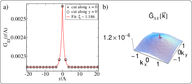
Figure 12: (Color online) a) The autocorrelation function of the non-affinity parameter $\chi$ for the harmonic triangular lattice with spring constant $\beta a^{2}f=200/\sqrt{3}$ in the $NpT$ ensemble with periodic boundary conditions along the $x$ and the $y$ axes. The red line is a fit to an exponential form. b) A surface plot of its Fourier transform $\tilde{G}_{\chi\chi}(\vec{k})$.

We have shown in this section that the coarse-graining process by which affine strains may be extracted from microscopic particle configurations also generates a random white noise consisting of non-affine particle displacements. For a harmonic solid this is simply related to the Lindemann parameter, which, in turn, depends ultimately on the strength of the interactions.

What is the general implication of this to the study of elasticity and rheology of complex solids? The current picture of the mechanism of relaxation in amorphous materials indicates that there are two main competing processes involved NGAI . Over small time scales the system fluctuates within local minima in the free energy landscape making transition between such basins of attraction over longer time scales. We have shown here that harmonic fluctuations within local minima generates a well characterized contribution to the non-affine displacement $\chi$, therefore any “extra” contribution to $\chi$ arises exclusively from these inter-basin transitions. Thus our analysis may be used as a tool to distinguish between these two kinds of relaxations in complex solids.

V Conclusions

We have shown in this paper how the analysis of particle configurations of two-dimensional soft solids gives access to a wealth of information on the local and non-local elastic properties. Since the harmonic solid analyzed here is the most generic conceivable our work has the potential to serve as a template for further research in this direction. The properties of the strain-strain correlation functions have been discussed in great detail and various methods of how to extract the elastic moduli from their analysis were presented. Furthermore we determined and discussed the effects of external pressure and an embedding medium, the proper treatment of which is essential for experimentalists seeking to use our methods for analyzing mechanical behavior of soft matter. The implications of our work particularly for the understanding of non-affineness in solids is significant, because our study allows one to classify non-affine fluctuations in any system into “trivial” (in the sense of being present even in an ideal harmonic solid) and non-trivial components. In the future, we shall use these procedures to study metastability in solids undergoing phase transitions and plastic behavior of solids under large external stresses.

- (1) A. Yethiraj, A. van Blaaderen, Nature, 421,513 (2003).
- (2) P. Habdas, E. R. Weeks, Curr. Opin. Colloid Interface Sci., 7, 196 (2002).
- (3) K.J. Strandburg, Rev. Mod. Phys., 60, 161 (1988); K.J Strandburg, ibid., 61, 747 (1989).
- (4) S. Sengupta, P. Nielaba and K. Binder, Phys. Rev. E, 61, 6294 (2000).
- (5) K. Binder, S. Sengupta and P. Nielaba, J. Phys.: Condens. Matter, 14, 2323 (2002).
- (6) H.H von Grünberg, P. Keim, K. Zahn and G. Maret, Phys. Rev. Lett., 93, 255703 (2004).
- (7) A. Wille, F. Valmont, K. Zahn and G. Maret, Europhys. Lett., 57, 219 (2002).
- (8) S. Sengupta, P. Nielaba, M. Rao and K. Binder, Phys. Rev. E, 61, 1072 (2000).
- (9) K. Zahn, A. Wille, G. Maret, S. Sengupta and P. Nielaba, Phys. Rev. Lett., 90, 155506 (2003).
- (10) R. Maranganti, P. Sharma, Phys. Rev. Lett., 98, 195504 (2007); R. Maranganti, P. Sharma, Journal of the Mechanics and Physics of Solids, 55, 1823 (2007).
- (11) K. Franzrahe, P. Keim, G. Maret, P. Nielaba and S. Sengupta, Phys. Rev. E, 78, 026106 (2008).
- (12) M.L. Falk, J.S. Langer, Phys. Rev. E, 57, 7192 (1998).
- (13) A. Lemaître, Phys. Rev. Lett., 89, 195503 (2002).
- (14) C.E. Maloney, M.O. Robbins, J. Phys.: Condens. Matter, 20, 244128 (2008).
- (15) P.M. Chaikin, T.C. Lubensky, Principles of condensed matter physics (Cambridge University Press, Cambridge, UK, 1995).
- (16) D.G.B. Edelen in Continuum Physics 4, A.C. Eringen, eds, (Academic Press, New York, 1976).
- (17) N. Goldenfeld, Lectures on Phase Transitions and the Renormalization Group (Westview Press, Boulder, Colorado, USA, 1992).
- (18) K. Franzrahe, P. Nielaba, A. Ricci, K. Binder, S. Sengupta, P. Keim and G. Maret, J. Phys.: Condens. Matter, 20, 404218 (2008).
- (19) P. Keim, G. Maret, U. Herz and H.H. von Grünberg, Phys. Rev. Lett., 92, 215504 (2004).
- (20) M. Parrinello, A. Rahman, J. Chem. Phys., 76, 2662 (1982).
- (21) D.R. Squire, A.C. Holt and W.G. Hoover, Physica, 42, 388 (1969).
- (22) D.C. Wallace, Thermodynamics of Crystals (Dover Publications Inc., Mineola, NY, 1998).
- (23) F. L. Román, J. A. White and S. Velasco, J. Chem. Phys., 107, 4635 (1997); F. L. Román, J. A. White, A. González, S. Velasco J. Chem. Phys., 110, 9821 (1999).
- (24) J. Lubliner, Plasticity Theory (Dover Publications Inc., Mineola, NY, 2008).
- (25) K. L. Ngai, G. B. Wright, eds, Relaxations in Complex Systems (NRL, Washington, DC, 1985).
- (26) H. Mori, Progress of Theoretical Physics, 33, 423 (1965).