Position-dependent exact-exchange energy for slabs and semi-infinite jellium

Abstract

The position-dependent exact-exchange energy per particle $\varepsilon_{x}(z)$ (defined as the interaction between a given electron at $z$ and its exact-exchange hole) at metal surfaces is investigated, by using either jellium slabs or the semi-infinite (SI) jellium model. For jellium slabs, we prove analytically and numerically that in the vacuum region far away from the surface $\varepsilon_{x}^{\text{Slab}}(z\rightarrow\infty)\rightarrow-\;e^{2}/2z$, independent of the bulk electron density, which is exactly half the corresponding exact-exchange potential $V_{x}(z\rightarrow\infty)\rightarrow-\;e^{2}/z$ [Phys. Rev. Lett. 97, 026802 (2006)] of density-functional theory, as occurs in the case of finite systems. The fitting of $\varepsilon_{x}^{\text{Slab}}(z)$ to a physically motivated image-like expression is feasible, but the resulting location of the image plane shows strong finite-size oscillations every time a slab discrete energy level becomes occupied. For a semi-infinite jellium, the asymptotic behavior of $\varepsilon_{x}^{\text{SI}}(z)$ is somehow different. As in the case of jellium slabs $\varepsilon_{x}^{\text{SI}}(z\rightarrow\infty)$ has an image-like behavior of the form $\propto-\;e^{2}/z$, but now with a density-dependent coefficient that in general differs from the slab universal coefficient $1/2$. Our numerical estimates for this coefficient agree with two previous analytical estimates for the same. For an arbitrary finite thickness of a jellium slab, we find that the asymptotic limits of $\varepsilon_{x}^{\text{Slab}}(z)$ and $\varepsilon_{x}^{\text{SI}}(z)$ only coincide in the low-density limit ($r_{s}\rightarrow\infty$), where the density-dependent coefficient of the semi-infinite jellium approaches the slab universal coefficient 1/2.

I Introduction

The jellium model of a metal surface, introduced by Bardeen in 1936, bardeen is the simplest model which reproduces qualitatively, and sometimes quantitatively, the physical properties of real metal surfaces. lang While in his work Bardeen applied an approximated Hartree-Fock (HF) theory for the study of the electronic structure, since the seminal work of Lang and Kohn (LK) langkohn the standard theoretical tool applied to the study of the electronic structure of metal surfaces has been Density-Functional Theory (DFT). dreizler As in the original work of Lang and Kohn, most of the subsequent investigations have applied the Local-Density Approximation (LDA) of DFT, or some of its semi-local variants (GGA, meta-GGA, etc.). This approach has been highly successful, and routinely yields good results for global surface properties such as work functions, surface energies, crystal-structure relaxation and reconstruction, etc. nekovee

At a more basic level, however, some problems still remain to be solved, concerning for instance the asymptotic behavior of the exchange-correlation (xc) potential of the widely used Kohn-Sham (KS) approach to DFT. In the LDA, this potential decays exponentially when evaluated in the vacuum region, instead of the expected image-like $\propto-\;e^{2}/z$ behavior. almbladh This qualitative failure of the LDA xc potential translates to a similar failure of the position-dependent xc energy per particle, $\varepsilon_{xc}({\bf r})$, which is defined through gunnarsson

$$E_{xc}[n]=\int n({\bf r})\;\varepsilon_{xc}({\bf r})\;d{\bf r},$$ (1)

with $E_{xc}[n]$ being the xc-energy contribution to the universal energy functional of DFT, and $n({\bf r})$ representing the electron density. Three aspects of Eq. (1) are worth emphasizing: (i) it represents the basic expression for the LDA, in which the exact $\varepsilon_{xc}({\bf r})$ of an arbitrary inhomogeneous electron system is replaced at each point ${\bf r}$ by that of a homogeneous electron gas at the local density $n({\bf r})$, and for a plethora of generalizations of the LDA, tao (ii) since $E_{xc}[n]$ can be split as the sum of exchange ($E_{x}[n]$) and correlation ($E_{c}[n]$) contributions, one can write $\varepsilon_{xc}({\bf r})=\varepsilon_{x}({\bf r})+\varepsilon_{c}({\bf r})$, and (iii) the position-dependent xc energy per particle $\varepsilon_{xc}({\bf r})$ entering Eq. (1) is not unique. One can always add to $\varepsilon_{xc}({\bf r})$ an arbitrary function $\varepsilon({\bf r})$ with the condition that weighted by the electron density $n({\bf r})$ integrates to zero. Here we have chosen $\varepsilon_{xc}({\bf r})$ to represent the interaction between a given electron at ${\bf r}$ and its xc hole.

The goal of this work is to provide exact analytical and numerical calculations of the exact-exchange $\varepsilon_{x}({\bf r})$ for jellium slabs and the semi-infinite (SI) jellium. In particular, we analyze the asymptotic behavior of the exact $\varepsilon_{x}({\bf r})$ in the vacuum region far away from the surface, and we find that there is a qualitative difference between $\varepsilon_{x}^{\text{Slab}}(z\rightarrow\infty)$ and $\varepsilon_{x}^{\text{SI}}(z\rightarrow\infty)$: both exhibit an image-like behavior of the form $-a\,e^{2}/z\,(a>0)$, but with a coefficient $a$ that while in the case of jellium slabs is universal and equal to 1/2 in the case of a semi-infinite jellium depends on the density of the bulk material and only approaches 1/2 in the low-density limit. The results reported here should help to settle the still controversial issue of the asymptotic behavior of the position-dependent xc energy per particle and KS xc potential at metal surfaces. gunnarsson ; ss ; ssb ; nastos

Besides, being the results presented here exact at the exchange level, they should also serve as a benchmark against to which DFT xc calculations could be confronted, and hopefully improved, once reduced to their exchange-only version. In this context, very recently Luo et al. luo have used a HF scheme to report self-consistent calculations of the surface energy and work function of jellium slabs.

The rest of the paper is organized as follows: In Section II we present the general theoretical background for both jellium slabs and the semi-infinite jellium, and we derive exact analytical expressions for the position-dependent exchange energy per particle in the vacuum region far away from the surface. Numerical calculations that are valid at all positions, from the bulk region to the vacuum, are reported in Section III. Section IV is devoted to the conclusions.

II Jellium slabs and the semi-infinite jellium: the exact asymptotic behavior

II.1 Jellium slabs

In the case of jellium slabs, with the discrete character of the positive ions inside the slab being replaced by a uniform distribution of positive charge (the jellium background), the positive jellium density is

$$n_{+}^{\text{Slab}}(z)=\overline{n}\,\theta(-z)\theta(d+z),$$ (2)

which describes a slab of width $d$, number density $\overline{n}$, note0 and jellium edges at $z=-d$ and $z=0$. $\theta(z)$ represents the Heaviside step function: $\theta(z)=1$ if $z>0$ and $\theta(z)=0$ if $z<0$. The size of the slab is infinite in the $x-y$ plane. The jellium slab is taken to be invariant under translations in the $x-y$ plane, so the KS eigenfunctions can be rigorously factorized as follows

$$\varphi_{i,{\bf k}}({\bf r})=\frac{e^{i{\bf k\cdot}\bm{\rho}}}{\sqrt{A}}\,\xi_{i}(z),$$ (3)

where $\bm{\rho}$ and ${\bf k}$ are the in-plane coordinate and wave-vector, respectively, and $A$ represents a normalization area in the $x-y$ plane. $\xi_{i}(z)$ are normalized spin-degenerate eigenfunctions for electrons in slab discrete levels (SDL) $i$ $(i=1,2,...)$ with energies $\varepsilon_{i};$ they are the solutions of the effective one-dimensional KS equation

$$\widehat{h}_{\text{KS}}^{i}(z)\xi_{i}(z)=\left[-\frac{\hbar^{2}}{2m_{e}}\frac{\partial^{2}}{\partial z^{2}}+V_{\text{KS}}\left(z\right)-\varepsilon_{i}\right]\xi_{i}(z)=0,$$ (4)

with $m_{e}$ being the electron mass. It is important to remark here that the factorization of the 3D wave-function as proposed in Eq. (3) is only valid for the case of a local potential, as is the case of the KS implementation of DFT. On the other hand, in the HF approximation the non-locality of the Fock potential introduces a coupling between ${\bf k}$ and $i$ quantum numbers luo . As a consequence, HF numerical calculations are more time-consuming than the ones presented here, either LDA, KLI KLI , or OEP. grabo

The local KS potential $V_{\text{KS}}(z)$ entering Eq. (4) is the sum of two distinct contributions:

$$V_{\text{KS}}(z)=V_{\text{H}}(z)+V_{xc}(z),$$ (5)

where $V_{\text{H}}(z)$ is the classical (electrostatic) Hartree potential, given by hartree.a

$$V_{\text{H}}(z)=-2\pi e^{2}\int_{-\infty}^{\infty}dz^{\prime}\left|z-z^{\prime}\right|\left[n^{\text{{Slab}}}(z^{\prime})-n_{+}(z^{\prime})\right].$$ (6)

Here, $n^{\text{Slab}}(z)$ is the electron number density dens.aa

$$n^{\text{Slab}}(z)=\frac{1}{2\pi}\sum_{i}^{occ.}\left(k_{F}^{i}\right)^{2}\left|\xi_{i}(z)\right|^{2},$$ (7)

where $k_{F}^{i}=\sqrt{2m_{e}(\varepsilon_{F}-\varepsilon_{i})}/\hbar$, and $\varepsilon_{F}=\varepsilon_{F}(\bar{n},d)$ is the Fermi energy or chemical potential, which in turn is determined from the neutrality condition for the whole system by the condition $\sum_{i}^{occ.}(k_{F}^{i})^{2}=2\pi\,d\,\overline{n}$. $V_{xc}(z)$ is the nonclassical xc potential, which is obtained as the functional derivative of the xc-energy functional $E_{xc}[n(z)]$: factor.a

$$V_{xc}(z)\equiv\frac{1}{A}\frac{\delta E_{xc}[n(z)]}{\delta n(z)}\;.$$ (8)

Both for the slab and semi-infinite [$d\rightarrow\infty$ limit of Eq. (2))] geometries, and as a consequence of the translational symmetry in the $x-y$ plane, Eq. (1) simplifies to

$$E_{xc}[n]=A\int\limits_{-\infty}^{\infty}dz\,n(z)\,\varepsilon_{xc}(z),$$ (9)

where $\varepsilon_{xc}(z)$ is the position-dependent xc energy per particle at plane $z$. In the case of jellium slabs, the exchange-only contribution to $E_{xc}[n]$ (which is originated in the Pauli exchange hole with all other correlation effects excluded) is known to be given by the following expression: reboredo

$$E_{x}^{\text{Slab}}[n]=-2e^{2}A\sum_{i,j}^{occ.}k_{F}^{i}k_{F}^{j}\int\limits_{-\infty}^{\infty}dz\int\limits_{-\infty}^{\infty}dz^{\prime}\varphi_{i}(z,z^{\prime})\varphi_{j}(z^{\prime},z)F_{ij}(z,z^{\prime}),$$ (10)

where $\varphi_{i}(z,z^{\prime})=\xi_{i}(z)^{*}\xi_{i}(z^{\prime})$ and

$$F_{ij}(z,z^{\prime})=\frac{1}{4\pi}\int\limits_{0}^{\infty}\frac{d\rho}{\rho}\frac{J_{1}(\rho k_{F}^{i})J_{1}(\rho k_{F}^{j})}{\sqrt{\rho^{2}+(z-z^{\prime})^{2}}}\;,$$ (11)

with $J_{1}(x)$ being the cylindrical Bessel function of first order. abra

Comparison of Eq. (9) and (10) yields the following expression for the exchange-only contribution to $\varepsilon_{xc}^{\text{Slab}}(z)$:

$$\varepsilon_{x}^{\text{Slab}}(z)=-\frac{2e^{2}}{n^{\text{Slab}}(z)}\sum_{i,j}^{occ.}k_{F}^{i}k_{F}^{j}\int\limits_{-\infty}^{\infty}dz^{\prime}\varphi_{i}(z,z^{\prime})\varphi_{j}(z^{\prime},z)F_{ij}(z,z^{\prime}),$$ (12)

which can be interpreted as the energy due to the interaction of an electron at $z$ and its exchange-only Pauli hole. In order to demonstrate that the exact-exchange energy per particle $\varepsilon_{x}^{slab}(z)$ of Eq. (12) represents indeed the interaction between an electron at $z$ and its exact-exchange hole, we appeal to the following expression for the exchange-hole for our slab geometryrrp

$$h_{x}({\bf r};{\bf r+R})=\frac{-1}{2(\pi\rho)^{2}n^{\text{Slab}}(z)}\sum_{i,j}^{occ.}k^{i}_{F}k^{j}_{F}J_{1}(\rho k^{i}_{F})J_{1}(\rho k^{j}_{F})\xi_{i}(z+Z)^{*}\xi_{i}(z)\xi_{j}(z+Z)\xi_{j}(z)^{*};,$$ (13)

which represents the density of the exchange hole at point ${\bf r+R}$ (observational point) due to the presence of an electron located at r. Owing to the translational symmetry in the $x-y$ plane, without loss of generality we have choose ${\bf r}=(0,z)$, ${\bf r+R}$ = ($\bm{\rho}$, $z+Z$). Using Eq. (13), and defining $z^{\prime}=z+Z$, Eq. (12) may be rewritten as

$$\varepsilon_{x}^{\text{Slab}}(z)=\frac{e^{2}}{2}\int d\bm{\rho}\int dz^{\prime}\frac{h_{x}(z;\rho,z^{\prime})}{\sqrt{\rho^{2}+(z-z^{\prime})^{2}}}\;,$$ (14)

which justifies the physical interpretation of $\varepsilon_{x}^{\text{Slab}}(z)$ as the interaction energy of an electron located at $z$ and the “charge distribution” given by $h_{x}(z;\rho,z^{\prime})$. Equations (13) and (14) can also be used as a sort of alternative definition of the $\varepsilon_{x}^{\text{Slab}}(z)$ investigated in this work, as they solve the non-uniqueness of $\varepsilon_{x}^{\text{Slab}}(z)$ which results from its definition through the exchange-only version of Eq. (9).tao01 ; tsp

II.1.1 Single occupied slab discrete level

In order to obtain the asymptotic behavior of $\varepsilon_{x}^{\text{Slab}}(z)$ at $z\rightarrow\infty$, we first restrict our analysis to the case where there is one single occupied SDL. oneSDL In this special case, in which $i=j=1$, Eq. (12) yields [see also Eqs. (7) and (11)]:

$$\varepsilon_{x,1}^{\text{Slab}}(z)=-\;e^{2}\;\int\limits_{-\infty}^{\infty}dz^{\prime}\left|\xi_{1}(z^{\prime})\right|^{2}\int\limits_{0}^{\infty}\frac{d\rho}{\rho}\frac{\left[J_{1}(\rho k_{F}^{1})\right]^{2}}{\sqrt{\rho^{2}+(z-z^{\prime})^{2}}},$$ (15)

or, equivalently (see Appendix):

$$\varepsilon_{x,1}^{\text{Slab}}(z)=-\frac{e^{2}}{2}\int\limits_{-\infty}^{\infty}dz^{\prime}\frac{\left|\xi_{1}(z^{\prime})\right|^{2}}{\left|z-z^{\prime}\right|}\left[1-\frac{I_{1}(2k_{F}^{1}\left|z-z^{\prime}\right|)}{k_{F}^{1}\left|z-z^{\prime}\right|}+\frac{L_{1}(2k_{F}^{1}\left|z-z^{\prime}\right|)}{k_{F}^{1}\left|z-z^{\prime}\right|}\right],$$ (16)

with $I_{1}$ and $L_{1}$ being the modified Bessel and Struve functions, respectively. abra

We note that Eq. (16) is valid for all $z,$ both inside and outside the jellium slab. Also, the cancellation of $n^{\text{Slab}}(z)$ which occurs in passing from Eq. (12) to Eq. (15) allows for the numerical calculation of $\varepsilon_{x,1}^{\text{Slab}}(z)$ for arbitrarily large values of $z$.

Asymptotic behavior.

For the slab geometry, it is permissible (and rigorous) to take the asymptotic limit $k_{F}^{1}\left|z-z^{\prime}\right|\simeq z\,k_{F}^{1}\gg 1,$ although the integral over $z^{\prime}$ runs from $-\infty$ to $+\infty.$ This is due to the fact that for a given $z$ the main contribution to the integral in Eq. (16) comes from values of $z^{\prime}$ inside the slab ($-d\lesssim z^{\prime}\lesssim 0$), as $\xi_{1}(z)$ decays exponentially one or two $\lambda_{F}$’s from each jellium edge.

At this point, we define $F(x)\equiv 1-I_{1}(2x)/x+L_{1}(2x)/x$ and use the asymptotic expansions of $I_{1}$ and $L_{1}$ in the limit $x\gg 1.$ We obtain abra

$$F(x\gg 1)\rightarrow 1-\frac{2}{\pi x}+\frac{1}{2x^{3}}-...\;\;.$$ (17)

Hence, as $z\,k_{F}^{1}\gg 1$, Eq. (16) yields the following asymptotic behavior:

$$\varepsilon_{x,1}^{\text{Slab}}(z\rightarrow\infty)\rightarrow-\frac{e^{2}}{2z}\left(1+\frac{\beta_{1}}{z}+\frac{\gamma_{1}}{z^{2}}+...\right),$$ (18)

where $\beta_{1}(d,r_{s})=\overline{z}^{1}(d,r_{s})-2/\left[\pi k_{F}^{1}(d,r_{s})\right]$ and $\gamma_{1}(d,r_{s})=\overline{z^{2}}^{1}(d,r_{s})-4\,\overline{z}^{1}/\left[\pi k_{F}^{1}(d,r_{s})\right]$, mean values being defined here as $\overline{O}^{i}=\int\xi_{i}(z)^{*}O(z)\,\xi_{i}(z)\,dz.$ The $r_{s}$ dependence of $\overline{z}^{1}(d,r_{s})$ and $\overline{z^{2}}^{1}(d,r_{s})$ comes from the self-consistent KS wave-functions $\xi_{i}(z)$, which for a given $d$ are different for different values of the slab density dictated by $r_{s}$. For details on the derivation of Eq. (18) from Eq. (16), we refer to the Appendix.

II.1.2 General situation

For the general situation where more than one SDL is occupied, we obtain the asymptotic limit of Eq. (12) by using the fact that for $z\rightarrow\infty$ (i) the electron density is dominated by the slowest decaying KS orbital, which corresponds to the highest occupied SDL ($i=m$), and (ii) the numerator of Eq. (12) is dominated by the term $i=j=m$, since all $\xi_{i}(z)$ with $i\neq m$ decay exponentially two or three $\lambda_{F}$’s from each jellium edge. Hence, in the vacuum region far away from the surface we find:

$$n^{\text{Slab}}(z\rightarrow\infty)\rightarrow\frac{(k_{F}^{m})^{2}}{2\pi}\left|\xi_{m}(z)\right|^{2}$$ (19)

and

$$\varepsilon_{x}^{\text{Slab}}(z\rightarrow\infty)\rightarrow-\frac{4\pi e^{2}}{\left|\xi_{m}(z)\right|^{2}}\int\limits_{-\infty}^{\infty}dz^{\prime}\varphi_{m}(z,z^{\prime})\varphi_{m}(z^{\prime},z)F_{mm}(z,z^{\prime}),$$ (20)

or, equivalently [see Eq. (11)]:

$$\varepsilon_{x}^{\text{Slab}}(z\rightarrow\infty)\rightarrow-\;e^{2}\int\limits_{-\infty}^{\infty}dz^{\prime}\left|\xi_{m}(z^{\prime})\right|^{2}\int\limits_{0}^{\infty}\frac{d\rho}{\rho}\frac{\left[J_{1}(\rho k_{F}^{m})\right]^{2}}{\sqrt{\rho^{2}+(z-z^{\prime})^{2}}}\;.$$ (21)

Finally, following the same procedure as in the case of a single occupied SDL, we find:

$$\varepsilon_{x}^{\text{Slab}}(z\rightarrow\infty)\rightarrow-\frac{e^{2}}{2z}\left(1+\frac{\beta_{m}}{z}+\frac{\gamma_{m}}{z^{2}}+...\right),$$ (22)

where $\beta_{m}(d,r_{s})=\overline{z}^{m}(d,r_{s})-2/\left[\pi k_{F}^{m}(d,r_{s})\right]$ and $\gamma_{m}(d,r_{s})=\overline{z^{2}}^{m}(d,r_{s})-4\,\overline{z}^{m}(d,r_{s})/\left[\pi k_{F}^{m}(d,r_{s})\right]$. note.bb

This result represents a straightforward generalization of the result presented above [Eq. (18)] for the case of one single occupied SDL. At this point, it is interesting to note that the leading contribution to $\varepsilon_{x}^{\text{Slab}}(z\rightarrow\infty)\rightarrow-\;e^{2}/2z$ can be easily obtained directly from Eqs. (15) or (21), by approximating the argument inside the square root by $z$ (in the large $z$ limit), and using the normalization of the KS orbitals $\xi_{i}(z)$ and the identity $\int\limits_{0}^{\infty}dxJ_{1}(x)^{2}/x=1/2$.

By considering a slab of thickness sufficiently large to make the energy spectrum continuous, Solamatin and Sahni ssb reached the conclusion that far away from the slab the so-called Slater potential $V_{S}(z)$ [which is twice the exchange energy per particle: $V_{S}(z)=2\varepsilon_{x}(z)$] decays as $-e^{2}/z^{2}$, in contrast with the asymptotic structure dictated by Eq. (22). This result is, however, not correct due to the fact that for a finite jellium slab (no matter how thick it is) the slab intrinsic discrete spectrum [corresponding to the eigenvalues $\varepsilon_{i}$ entering Eq. (4)] can never be replaced by a continuous one.

Equation (22) leads us to the conclusion that in the vacuum region of a finite jellium slab and at distances from the surface that are large compared to $1/k_{F}^{m}$ (which is typically larger than the slab thickness $d$), $\varepsilon_{x}^{\text{Slab}}(z\rightarrow\infty)\rightarrow-\;e^{2}/2z$, which is exactly half the corresponding KS exact-exchange potential $V_{x}(z\to\infty)\rightarrow-\;e^{2}/z$.hpr Hence, as in the case of finite systems,gllb the Slater potential $V_{S}(z)$ of jellium slabs [or, equivalently, twice the exchange-energy per particle $\varepsilon_{x}(z)$] embodies the asymptotics of the KS exchange potential $V_{x}(z)$.

In contrast, Solamatin and Sahni ss ; ssb concluded that in the case of a semi-infinite jellium only half the Slater potential embodies the asymptotics of the KS exchange potential, i.e., $V_{x}(z\to\infty)=\varepsilon_{x}(z\to\infty)$; but Nastos nastos claimed that $V_{x}(z\to\infty)=2\varepsilon_{x}(z\to\infty)$, so there is still something remaining to be clarified on this issue. Work along these lines is now in progress.notesahni0

II.2 Two-dimensional electron gas

The exchange energy of a strict two-dimensional (2D) electron gas can be obtained from that of a jellium slab with a single occupied SDL [Eq. (10) with $i=j=1$], by first performing the one-dimensional non-uniform scaling pollak

$$n_{\lambda}^{\text{Slab}}(z)=\lambda\;n^{\text{Slab}}(\lambda z)\;,$$ (23)

and then taking the limit as $\lambda\to\infty$. The scaling above preserves the total number of electrons. Noting that for a single occupied SDL the jellium-slab exchange energy takes the following form

$$E_{x}^{\text{Slab}}[n]=-\frac{2\pi e^{2}A}{\left(k_{F}^{1}\right)^{2}}\int\limits_{0}^{\infty}\frac{d\rho}{\rho}\left[J_{1}(k_{F}^{1}\rho)\right]^{2}\int\limits_{-\infty}^{\infty}dz\int\limits_{-\infty}^{\infty}dz^{\prime}\frac{n^{\text{Slab}}(z)\;n^{\text{Slab}}(z^{\prime})}{\sqrt{\rho^{2}+(z-z^{\prime})^{2}}},$$ (24)

where

$$n^{\text{Slab}}(z)=\frac{\left(k_{F}^{1}\right)^{2}}{2\pi}\left|\xi_{1}(z)\right|^{2},$$ (25)

we find:

$$E_{x}^{\text{2D}}\equiv\lim_{\lambda\to\infty}E_{x}^{\text{Slab}}[n_{\lambda}^{\text{Slab}}]=-N\,\frac{4}{3\pi}e^{2}\;k_{F}^{1},$$ (26)

where $N=A\left(k_{F}^{1}\right)^{2}/(2\pi)$ represents the total number of electrons. Previously, this scaling limit had been formulated in a different way, resulting in the much generous constraint that the exchange energy per particle in the 2D ($\lambda\rightarrow\infty$) limit should be greater than $-\;\infty$. pollak ; cpp ; constantin It is interesting to note that the exchange energy functional as given by Eq. (24) is an explicit functional of the density, which is only possible in this single occupied SDL case, due to the simple (invertible) relation between density and wave-function, as given by Eq. (25). In the general, many SDL occupied case, Eq. (25) is replaced by Eq. (7), the direct inversion from wave-functions to density is not feasible anymore, and the exchange energy functional is an explicit functional of the KS orbitals, but an implicit functional of the density, as in Eq. (10).

We note at this point that the exchange energy of a strict 2D electron gas can also be obtained directly from Eq. (15) through the replacement $\xi_{1}(z^{\prime})\rightarrow\sqrt{\delta(z^{\prime})},$ with $\delta(z^{\prime})$ being the Dirac delta function, and taking $z=0$:

$$E_{x}^{\text{2D}}=-N\,e^{2}\int\limits_{0}^{\infty}\frac{d\rho}{\rho^{2}}\,\left[J_{1}(\rho k_{F}^{1})\right]^{2}=-N\,\frac{4}{3\pi}e^{2}k_{F}^{1}.$$ (27)

Either from Eq. (26) or (27), we find for the exchange energy per particle of the strict 2D homogeneous electron gas the well-known result $\varepsilon_{x}^{\text{2D}}=E_{x}^{\text{2D}}/N=-(4/3\pi)e^{2}k_{F}^{1}\;$. GV

II.3 Semi-infinite jellium

In the case of a semi-infinite jellium, a half-space filled with a uniform distribution of positive charge (the jellium background), the jellium density is

$$n_{+}^{\text{SI}}(z)=\overline{n}\,\theta\left(-z\right),$$ (28)

with the jellium edge at $z=0$ defining the surface of a metal. As in the case of jellium slabs, the semi-infinite jellium is invariant under translations in the $x-y$ plane, so the KS eigenfunctions can be factorized as follows

$$\varphi_{k_{z},{\bf k}}({\bf r})=\frac{e^{i{\bf k\cdot}\bm{\rho}}}{\sqrt{A}}\,\frac{\xi_{k_{z}}(z)}{\sqrt{L}},$$ (29)

where $\bm{\rho}$ and ${\bf k}$ are the in-plane coordinate and wave-vector, respectively, and $A$ ($L$) represents a normalization area (length). $\xi_{k_{z}}(z)$ are spin-degenerate eigenfunctions for electrons with a continuous energy spectrum $\varepsilon_{k_{z}}=V_{\text{KS}}(-\infty)+(\hbar k_{z})^{2}/2m_{e}$ ($k_{z}$ is a continuum quantum number). They are the solutions of the effective one-dimensional KS equation

$$\widehat{h}_{\text{KS}}^{k_{z}}(z)\xi_{k_{z}}(z)=\left[-\frac{\hbar^{2}}{2m_{e}}\frac{\partial^{2}}{\partial z^{2}}+V_{\text{KS}}\left(z\right)-\varepsilon_{k_{z}}\right]\xi_{k_{z}}(z)=0.$$ (30)

The KS potential $V_{\text{KS}}(z)$ is given by Eq. (5), as in the case of a jellium slab but with the slab electron density of Eq. (7) being replaced by the SI electron density

$$n^{\text{SI}}(z)=\frac{1}{4\pi^{2}}\int\limits_{-k_{F}}^{k_{F}}(k_{F}^{2}-k_{z}^{2})\left|\xi_{k_{z}}(z)\right|^{2}dk_{z}.\\$$ (31)

In the case of a semi-infinite jellium, the position-dependent exchange energy per particle at plane $z$ is given by the following expression:

$$\varepsilon_{x}^{\text{SI}}(z)=-\frac{e^{2}}{2\pi^{2}n^{\text{SI}}(z)}\int\limits_{-k_{F}}^{k_{F}}dk_{z}\int\limits_{-k_{F}}^{k_{F}}dk_{z}^{{}^{\prime}}(k_{F}^{2}-k_{z}^{2})^{1/2}(k_{F}^{2}-k_{z}^{{}^{\prime}2})^{1/2}\int\limits_{-\infty}^{\infty}dz^{\prime}\varphi_{k_{z}}(z,z^{\prime})\varphi_{k_{z}^{{}^{\prime}}}(z^{\prime},z)F_{k_{z}k_{z}^{{}^{\prime}}}(z,z^{\prime}),$$ (32)

where $\varphi_{k_{z}}(z,z^{\prime})=\xi_{k_{z}}(z)^{*}\xi_{k_{z}}(z^{\prime})$, and $F_{k_{z}k_{z}^{{}^{\prime}}}(z,z^{\prime})$ is of the form of Eq. (11) but with $k_{F}^{i}$ ($k_{F}^{j}$) being replaced by $[k_{F}^{2}-k_{z}^{2}]^{1/2}$ ($[k_{F}^{2}-k_{z}^{{}^{\prime}2}]^{1/2}$).

Asymptotic behavior.

The derivation of the asymptotic limit of $\varepsilon_{x}^{\text{SI}}(z)$ is more delicate than in the case of jellium slabs, due to the fact that in the present case we have a continuous energy spectra. Hence, the crucial argument that we have used to derive the asymptotic behavior for jellium slabs, concerning the fact that in that case the highest occupied SDL dominates in the vacuum region far away from the surface, is not so transparent when the spectrum is continuous. Stated in other words, contributions to the asymptotic position-dependent exchange energy of Eq. (32) come indeed from values of $k_{z}$ and $k_{z}^{{}^{\prime}}$ that approach $k_{F}$, but not necessarily only from the highest occupied value, i.e., from $k_{z}=k_{z}^{{}^{\prime}}=k_{F}$.

The asymptotic behavior of Eq. (32) was analyzed by Nastos nastos by assuming that at $z\to\infty$ the KS potential $V_{\text{KS}}(z)$ takes the image-like form $V_{\text{KS}}(z\rightarrow\infty)\rightarrow-\;\alpha_{\text{KS}}\,e^{2}/z$, with $\alpha_{\text{KS}}$ positive, but otherwise arbitrary. One finds that in the vacuum region far away from the surface ($z\rightarrow\infty$) the KS orbitals $\xi_{k_{z}}$ can be expanded with respect to the KS orbital at $k_{z}=k_{F}$ as followsnastos ; qs

$$\xi_{k}(z\rightarrow\infty)\rightarrow\xi_{k_{F}}(z\rightarrow\infty)e^{-\alpha z(k_{F}-k)}\;,$$ (33)

with

$$\xi_{k_{F}}(z\rightarrow\infty)\propto e^{-z\sqrt{2m_{e}W/\hbar^{2}}}(2z\sqrt{2W})^{\alpha_{\text{KS}}/\sqrt{2m_{e}a_{0}^{2}W/\hbar^{2}}},$$ (34)

$\alpha$ standing for the square root of the ratio between the Fermi energy and the work function $W$ ($\alpha^{2}=\varepsilon_{F}/W$). By introducing Eqs. (33) and (34) into Eqs. (31) and (32), one findsnastos ; qs

$$n^{\text{SI}}(z\rightarrow\infty)\rightarrow\frac{3\overline{n}}{4(\alpha k_{F}z)^{2}}\left|\xi_{k_{F}}(z\rightarrow\infty)\right|^{2}\;,$$ (35)

and

$$\varepsilon_{x}^{\text{SI}}(z\rightarrow\infty)\rightarrow-\frac{\pi+2\alpha\ln(\alpha)}{2\pi(1+\alpha^{2})}\frac{e^{2}}{z}.$$ (36)

Furthermore, the asymptote of Eq. (36) does not depend on the actual form of $\xi_{k_{F}}(z\rightarrow\infty)$. This is due to a cancellation, when $z$ is large, of the orbitals $\xi_{k_{F}}(z\rightarrow\infty)$ entering the numerator and denominator of Eq. (32). This is the reason why the leading term in the expansion of $\varepsilon_{x}^{\text{SI}}(z\rightarrow\infty)$ is independent of $\alpha_{\text{KS}}$. That means that the result remains valid also in the absence of this image-like contribution, i.e., even assuming that the KS potential $V_{\text{KS}}(z)$ entering Eq. (4) decays exponentially as $z\rightarrow\infty$.

The asymptotic behavior dictated by Eq. (36) was obtained independently by Solamatin and Sahni using a somehow less general, but otherwise quite different approach. ss ; ssb ; notesahni They approximated the KS potential $V_{\text{KS}}(z)$ entering Eq. (30) by a finite-linear-potential model at the interface region, and used the corresponding orbitals in each of the three regions where the model was defined: trigonometric functions (in the bulk region), Airy functions (near the surface), and exponential decaying functions (in the vacuum). As the only thing that matters in obtaining the asymptote of Eq. (36) is the correct expansion of the KS orbitals with respect to the KS orbital at $k_{z}=k_{F}$ [as given by Eq. (33)], and with this general expansion being fulfilled also within the finite-linear-model potential used in Refs. ss, and ssb, , Solamatin and Sahni obtained Eq. (36) which is valid in general. It is also worth of address the fact that the result of Eq. (36) is in contrast with the asymptotic behavior $\varepsilon_{x}(z\rightarrow\infty)\rightarrow-\;e^{2}/4z$ that one obtains for the exchange energy per particle in the case of the Airy edge electron gas. KM This is due to the fact that the asymptotic behavior of the solutions of the Airy edge gas is different from the one given by Eq. (33), as for this model the potential increases linearly with distance in the vacuum region, instead of approaching a constant value. An analysis of the so-called Pauli and lowest-order correlation-kinetic components of the exchange energy per particle $\epsilon_{x}(z\to\infty)$ can be found in Ref. qs, .

III Numerical results

All the numerical calculations presented below have been carried out by ignoring all correlation effects (beyond the Pauli exchange). By this we mean that the xc potential $V_{xc}(z)$ entering Eq. (4) has been replaced by the exchange-only contribution $V_{x}(z)$, disregarding $V_{c}(z)$, both for jellium slabs and for the semi-infinite jellium. In the case of jellium slabs, $V_{x}(z)$ and the corresponding KS orbitals of Eq. (4) can be obtained through the solution of the discrete version of the $x$-only optimized effective potential (OEP) method, as given for example by Eqs. (14) or (20) of Ref. hpp, . This code is feasible and we have at our disposal these self-consistent exact-exchange (OEP) KS orbitals and exchange potentials. hpp ; hpr Alternatively, an approximate way to obtain $V_{x}(z)$ and the corresponding KS orbitals (the exchange-only LDA orbitals) is to replace the actual exchange potential $V_{x}(z)$ by the exchange potential of a uniform electron gas at the local electron density $n(z)$, i.e., $V_{x}^{\text{LDA}}(z)=-\left[6n(z)/\pi\right]^{1/3}$ [hartrees].

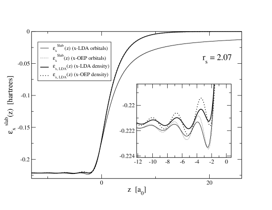
Figure 1: $\varepsilon_{x}^{\text{Slab}}(z)$ for $r_{s}=2.07$ and slab width $d=4.3\;\lambda_{F}$. The curves denoted “Slab” have been evaluated from Eq. (12), by using exchange-only LDA orbitals (solid line) and exact-exchange (OEP) orbitals (dotted line). The curves denoted ”LDA” have been evaluated from the well-known LDA formula $\varepsilon_{x,\text{LDA}}(z)=-(3/4\pi)[3\pi^{2}n(z)]^{1/3}$ [hartrees], with $n(z)$ being the exchange-only self-consistent electron density obtained with the use of exchange-only LDA orbitals (wide solid line) and exact-exchange (OEP) orbitals (wide dotted line). Inset: enlarged view of the bulk region near the surface. The bulk value of $\varepsilon_{x}$ for this electron density is $-\;0.22134\;(e^{2}/a_{0})$.

Fig. 1 shows a comparison of (i) the well-known LDA exchange energy per particle $\varepsilon_{x,\text{LDA}}(z)=-(3/4\pi)\left[3\pi^{2}n(z)\right]^{1/3}$ [hartrees], with $n(z)$ being the self-consistent electron density obtained with the use of either exchange-only LDA orbitals (wide solid line) or exact-exchange (OEP) orbitals (wide dotted line), with (ii) the exact-exchange energy per particle $\varepsilon_{x}^{\text{Slab}}(z)$ of Eq. (12) obtained by using, as before, either exchange-only LDA orbitals (solid line) or exact-exchange (OEP) orbitals (dotted line). It is important to note that while both alternative evaluations of $\varepsilon_{x,\text{LDA}}(z)$ fail badly in the vacuum region where the actual exchange energy per particle exhibits an image-like asymptotic behavior, the use of LDA orbitals in Eq. (12) results in an exchange energy per particle (solid line) that on the scale of the figure is nearly identical to the exact fully-self-consistent result (dotted line). Small differences introduced by the use of LDA orbitals (see the inset) are mostly localized in the bulk region near the surface, where Friedel-like oscillations appear to be too weak in this approximation.

The numerical methods that we have used to obtain exact-exchange (OEP) orbitals and exchange-only LDA orbitals suffer from instabilities in the vacuum region far from the surface. As in this region exchange-only LDA orbitals are stabler than their OEP counterparts and the results presented in this work do not depend significantly on whether exact-exchange (OEP) or exchange-only LDA orbitals are used in Eq. (12) (see Fig. 1), all the calculations presented below have been obtained with the use of exchange-only LDA orbitals. We emphasize, however, that this is not a crucial approximation, and that the magnitude of the error that it introduces is given by the almost indistinguishable difference between the full and dotted lines in Fig. 1.

The numerical self-consistent calculations presented in Fig. 1 and in the remaining of this section (which are all obtained from either Eq. (12) or Eq. (32) with the use of exchange-only LDA orbitals) have been performed as follows. For jellium slabs, two infinite barriers have been located in the vacuum region far enough away from the two surfaces, in such a way that all the numerical results be independent of their precise location, note0a and the KS equations have been solved through a straightforward discretization in real space along the one-dimensional coordinate $z$. In the case of the semi-infinite jellium, the KS equations have been solved by following the general procedure introduced by Lang and Kohn. langkohn This consists of defining three regions for the solution of the KS equation: far-left (bulk region), central (a few $\lambda_{F}$’s to the left and to the right of the jellium edge), and far-right (vacuum region). In the bulk region, the KS eigenfunctions are taken to be of the form $\xi_{k}(z)=\sin(kz-\gamma_{k})$, where $\gamma_{k}$ are phase shifts, and this fixes an overall normalization constant. In the central region, we define a mesh of $N$ points between $z_{1}$ and $z_{N}$ $(z_{1}<z_{N})$, the first point $z_{1}$ being chosen far enough from the jellium edge in the bulk so that the Friedel oscillations can be neglected, and the outer point $z_{N}$ being chosen to be far enough from the jellium edge into the vacuum so that the effective one-electron potential is negligibly small. Since $V_{\text{KS}}(z)\sim 0$ for $z\geq z_{N}$, the orbitals can be approximated as $\xi_{k}(z_{N})=a\,e^{-k^{*}z}$ where $a$ is a constant and $k^{*}=(-2m_{e}\varepsilon_{k_{z}}/\hbar^{2})^{1/2}$. The KS orbitals at the mesh points are calculated by using the Numerov integration procedure. liebsch As in the vacuum region the orbitals follow exponential form, it is numerically most stable to integrate them inwards, so the Numerov integration procedure in this case is given by:

$$\xi_{k}(z_{i-1})=\frac{2+10h(V_{\text{KS}}(z_{i})-\varepsilon_{k_{z}})}{1-h(V_{\text{KS}}(z_{i-1})-\varepsilon_{k_{z}})}\xi_{k}(z_{i})-\frac{1-h(V_{KS}(z_{i+1})-\varepsilon_{k_{z}})}{1-h(V_{\text{KS}}(z_{i-1})-\varepsilon_{k_{z}})}\xi_{k}(z_{i+1}),$$ (37)

where $h=(z_{i+1}-z_{i})^{2}/12$. Finally, matching the KS orbitals in the central region with the corresponding analytical expression in the bulk region [$\xi_{k}(z)=\sin(kz-\gamma_{k})$] determines the constant $a$.

III.1 Jellium slabs

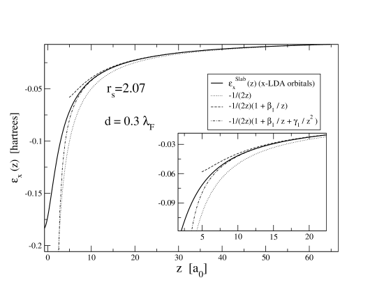
Figure 2: Position-dependent exchange-energy per particle for a thin jellium slab with $r_{s}=2.07$ and $d=0.3\;\lambda_{F}\approx 2a_{0}$. Solid line: full numerical calculation of Eq. (12). Dashed-dotted lines: asymptote of Eq. (18); the dashed (dotted) lines represent the asymptote of Eq. (18) with the last term (last two terms) neglected. Inset: enlarged view of the asymptotic region.

In Fig. 2, we consider a thin jellium slab with $r_{s}=2.07$ (corresponding to the average electron density of Al) and $d=0.3\,\lambda_{F}$. This slab contains one single occupied SDL, so that we compare our full numerical calculation of Eq. (12) (solid line) with the asymptote of Eq. (18) (dashed-dotted line). We see that $\varepsilon_{x}^{\text{Slab}}(z)$ reaches Eq. (18) at about one $\lambda_{F}$ from the jellium edge and reaches the asymptote $-e^{2}/2z$ at a few Fermi wavelengths ($\sim 5-6\lambda_{F}$) from the surface.

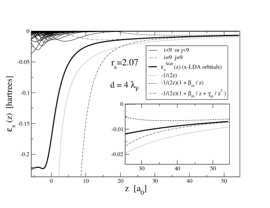
Figure 3: Same as Fig. 2, but for a slab with $d=4\;\lambda_{F}$, with nine SDL occupied. Full thick line, $\varepsilon_{x}^{\text{Slab}}(z)$ from Eq. (12); dotted, dashed, and dashed-dotted lines, asymptotic expansions from Eq. (22). The contribution from each pair $(i,j)$ of occupied SDL to the total ${\varepsilon_{x}}^{\text{Slab}}(z)$ are represented with thin full lines, except for the last contribution ($i=j=9$). Inset: enlarged view of the asymptotic region.

In Fig. 3, we consider a jellium slab with $r_{s}=2.07$ and $d=4\,\lambda_{F}$. For this particular case, nine SDL’s are occupied, i.e., $\varepsilon_{9}<\varepsilon_{F}<\varepsilon_{10}$, so we compare our full numerical calculation of Eq. (12) (solid line) with the asymptote of Eq. (22) (dashed-dotted line). The main message of this figure is that (i) in the vacuum region far away from the surface $\varepsilon_{x}^{\text{Slab}}(z)$ is dominated by the term $i=j=m$ (dashed-dotted-dotted line), and (ii) $\varepsilon_{x}^{\text{Slab}}(z)$ reaches the asymptote $-e^{2}/2z$ only at a distance from the jellium edge of several Fermi wavelengths ($\sim 8\lambda_{F}$). We remind here that point (i) above was our main assumption in the derivation of the slab asymptotic limit of Eq. (22). This assumption is fully justified after the numerical results shown in Fig. 3.

At this point, with a few algebraic manipulations, we rewrite the asymptote of Eq. (22) in the physically motivated image-like form

$$\varepsilon_{x}^{\text{Slab}}(z\rightarrow\infty)\rightarrow-\;\alpha_{x}^{\text{Slab}}\frac{e^{2}}{\left[z-z_{x}^{\text{Slab}}(d,r_{s},z)\right]},$$ (38)

where

$$\alpha_{x}^{\text{Slab}}=1/2,$$ (39)

and $z_{x}^{\text{Slab}}(d,r_{s},z)$, which represents the location of the so-called image plane, results in

$$z_{x}^{\text{Slab}}(d,r_{s},z)=\beta_{m}(d,r_{s})+\frac{\gamma_{m}(d,r_{s})-[\beta_{m}(d,r_{s})]^{2}}{z}+O\left(\frac{1}{z^{2}}\right).$$ (40)

As $z\rightarrow\infty$, $z_{x}^{\text{Slab}}(d,r_{s},z)$ reaches a finite value, given by

$$z_{x}^{\text{Slab}}(d,r_{s},z\rightarrow\infty)\rightarrow\beta_{m}(d,r_{s})=\overline{z}^{m}(d,r_{s})-2/\pi k_{F}^{m}(d,r_{s})=-d/2-2/\pi k_{F}^{m}(d,r_{s}).$$ (41)

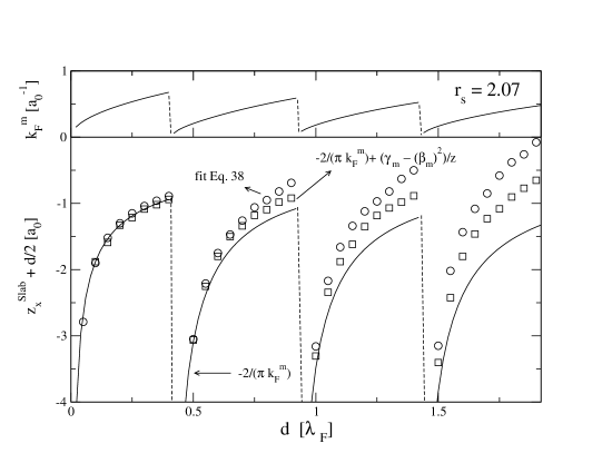
Figure 4: Parameter $z_{x}^{\text{Slab}}(d,r_{s}=2.07,z)$ from Eq. (38), as a function of $d$, in several approximations. Full line, $z_{x}^{\text{Slab}}(d,r_{s}=2.07,z\rightarrow\infty)+d/2=-2/\pi k_{F}^{m}(d,r_{s}=2.07)$; squares, Eq. (40); circles, fit to Eq. (38). Upper panel, $k_{F}^{m}(d)$ as a function of $d$.

In Fig. 4, we plot a comparison of Eq. (41) (solid line) with the image-plane position that we obtain by fitting our full numerical calculation of Eq. (12) with the image-like Eq. (38) and $\alpha_{x}^{\text{Slab}}=1/2$ (empty circles). For this, we have used a fit region of width $2\lambda_{F}$ centered at $6\lambda_{F}$ from the jellium edge in the vacuum. Differences between Eq. (41) (solid line) and our numerical estimate (empty circles), which in the case of very thin films are negligible, are entirely due to the fact that the fitting of the numerical calculation must be carried out in a vacuum region that extends very far away from the surface. Empty squares correspond to the result of Eq. (40), including the correction to the leading term, and taking $z=6\lambda_{F}$ (which is the average value of the fit region indicated above). According to Eq. (41), $z_{x}^{\text{Slab}}(d)+d/2$ is inversely proportional to $k_{F}^{m}(d)$, which exhibits an oscillatory behavior as a function of the slab width $d$ (see the solid line in the upper part of Fig. 4) going to zero every time a SDL becomes occupied. Hence, the location of the image plane becomes infinitely negative every time a SDL becomes occupied, which results in the strong finite-size oscillations shown in Fig. 4.

III.2 Semi-infinite jellium

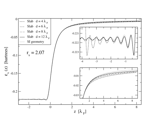
Figure 5: $\varepsilon_{x}^{\text{Slab}}(z)$ for $r_{s}=2.07$, slabs with $d=4,6,8$, and $12\;\lambda_{F}$. Dotted line, $\varepsilon_{x}^{\text{SI}}(z)$ for the semi-infinite case, from Eq. (32). Upper inset: enlarged view of the bulk region. Lower inset: asymptotic region.

Now we focus on a comparison between our full numerical jellium-slab and semi-infinite-jellium calculations of the position-dependent exchange energy per particle (see Fig. 5). In the bulk, as $d$ increases the slab calculations converge with the semi-infinite calculation (see the inset at the upper part of Fig. 5), and both slab and semi-infinite calculations approach in the bulk region far away from the surface the exchange energy per particle of a three-dimensional (3D) homogeneous electron gas, $\varepsilon_{x}^{\text{3D}}/(e^{2}/a_{0})=-(3/4\pi)(9\pi/4)^{1/3}/r_{s}\approx-\;0.22134$. In the vacuum, however, there is always a region far enough away from the surface where the jellium slab and the semi-infinite jellium behave differently: while all slab calculations converge to an image-like behavior of the form of Eq. (38) with $\alpha_{x}^{\text{Slab}}=1/2$, the semi-infinite $\varepsilon_{x}^{\text{SI}}(z\rightarrow\infty)$ exhibits an image-like behavior in agreement with Eq. (36) (see Fig. 6). Fig. 5 also shows that as the width $d$ increases the slab $\varepsilon_{x}^{\text{Slab}}(z)$ coincides with the semi-infinite $\varepsilon_{x}^{\text{SI}}(z)$ in a wider vacuum region near the surface (see the lower inset of Fig. 5).

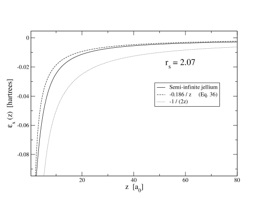
Figure 6: Asymptotic behavior of $\varepsilon_{x}^{\text{SI}}(z)$ for the semi-infinite case, and comparison with Eq. (36) and the asymptote form of Eq. (22).

Fig. 6 shows a comparison of our full numerical calculation of Eq. (32) with the asymptote of Eq. (36) (solid and dashed lines, respectively) for $r_{s}=2.07$. In this case, $\alpha=\sqrt{\varepsilon_{F}/W}=2.048$ (as obtained from our exchange-only LDA self-consistent calculation of the work function $W$) and Eq. (36) yields $\varepsilon_{x}^{\text{SI}}(z\rightarrow\infty)\rightarrow-0.18622\;e^{2}/z$ (dashed line), which is in contrast with the asymptote of Eq. (22) (dotted line) that holds in the case of jellium slabs. The same comparison has been done for other values of $r_{s}$, and we have found that our full numerical calculation is always very close (as in Fig. 6) to the asymptote of Eq. (36).

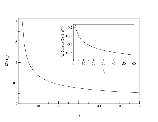
Figure 7: $\alpha(r_{s})=\sqrt{\varepsilon_{F}(r_{s})/W(r_{s})}$ versus $r_{s}$, for the semi-infinite case. Inset, the coefficient $-\left[\pi+2\alpha\ln(\alpha)\right]/\left[2\pi(1+\alpha^{2})\right]$ of Eq. (36) versus $r_{s}$.

Finally, we display in Fig. 7 our exchange-only LDA self-consistent calculation of the coefficient $\alpha=\sqrt{\varepsilon_{F}/W}$ in a wide range of electron densities. It is important to note that the corresponding coefficient $\left[\pi+2\alpha\ln(\alpha)\right]/\left[2\pi(1+\alpha^{2})\right]$ (see the inset to Fig. 7) entering Eq. (36) is close to $1/4$ at metallic densities ($r_{s}=2-6$). Fig. 7 also shows that only at extremely low densities the coefficient $\alpha$ approaches zero, thereby the coefficient $\left[\pi+2\alpha\ln(\alpha)\right]/\left[2\pi(1+\alpha^{2})\right]$ of Eq. (36) approaching $1/2$. Hence, the asymptotic limits of $\varepsilon_{x}^{\text{Slab}}(z)$ and $\varepsilon_{x}^{\text{SI}}(z)$ only coincide in the low-density limit ($r_{s}\to\infty$).

IV Summary and conclusions

We have presented a detailed analysis of the position-dependent exchange energy per particle $\varepsilon_{x}(z)$ at jellium slabs and the semi-infinite jellium.

For jellium slabs, we have found that in the vacuum region far away from the surface $\varepsilon_{x}^{\text{Slab}}(z\rightarrow\infty)\rightarrow-\;e^{2}/(2z)$, independent of the bulk electron density. This is the equivalent to the well-known result $\varepsilon_{x}({\bf r}\rightarrow\infty)\rightarrow-\;e^{2}/(2r)$, which holds in the case of localized finite systems like atoms and molecules. dreizler The equivalence between these results is however not straightforward, since slabs have an extended character in the $x-y$ plane, being “localized” only along the $z$-coordinate. In the vacuum side of the surface there is a region where $\varepsilon_{x}^{\text{Slab}}(z)$ coincides with $\varepsilon_{x}^{\text{SI}}(z)$ and this region increases as $d$ increases. The fitting of our numerical calculations of $\varepsilon_{x}^{\text{Slab}}(z)$ to a physically motivated image-like expression is feasible, but the resulting location of the image plane $[z_{x}^{\text{Slab}}(d,r_{s},z)]$ shows strong finite-size oscillations. In particular, we have shown analytically that $z_{x}^{\text{Slab}}(d,r_{s},z\rightarrow\infty)=-d/2-2/\pi k_{F}^{m}(d,r_{s})$, $k_{F}^{m}(d,r_{s})$ being a signature of the energy of the highest occupied SDL with respect to the Fermi level.

For a semi-infinite jellium, we have found that our numerical calculations agree well with the analytical asymptote [see Eq. (36)] obtained in Refs. ss, ; ssb, ; nastos, and qs, , which approaches the slab asymptote $-\;e^{2}/2z$ only in the extreme low-density limit ($r_{s}\to\infty$).

We attribute the qualitatively different behavior of $\varepsilon_{x}^{\text{Slab}}(z\rightarrow\infty)$ and $\varepsilon_{x}^{\text{SI}}(z\rightarrow\infty)$ to the fact that these asymptotes are approached in different ranges. While in the case of the semi-infinite jellium the asymptote is reached at distances $z$ from the surface that are large compared to the Fermi wavelength (the only existing length scale in this model), for slabs the asymptote is reached at distances $z$ from the surface that are large compared to $1/k_{F}^{m}$ (which is typically larger than the slab thickness $d$). For thick slabs with $d>>\lambda_{F}$ ($\lambda_{F}$ being the Fermi wavelength), $\varepsilon_{x}^{\text{Slab}}(z)$ first coincides with $\varepsilon_{x}^{\text{SI}}(z)$ [dictated by Eq. (36) at $z>>\lambda_{F}$] in the vacuum region near the surface (see Fig. 5), but at distances from the surface that are large compared to $1/k_{F}^{m}$, $\varepsilon_{x}^{\text{Slab}}(z)$ turns to the slab image-like behavior of the form of Eq. (22) [or, equivalently, Eq. (38) with $\alpha_{x}^{\text{Slab}}=1/2$]; in the limit as $d\to\infty$ (i.e., when the jellium slab becomes semi-infinite), $\varepsilon_{x}^{\text{Slab}}(z\to\infty)$ coincides with $\varepsilon_{x}^{\text{SI}}(z\to\infty)$ everywhere. In the low-density limit, where $\lambda_{F}\to\infty$, the condition $d>>\lambda_{F}$ is never fulfilled and $\varepsilon_{x}^{\text{Slab}}(z)$ reaches (at $z>>1/k_{F}^{m}$) one single asymptote: the slab image-like behavior of the form of Eq. (22) [or, equivalently, Eq. (38) with $\alpha_{x}^{\text{Slab}}=1/2$], which turns out to coincide with the semi-infinite-jellium asymptotic behavior dictated by Eq. (36).

Finally, we note that as $\varepsilon_{xc}(z)=\varepsilon_{x}(z)+\varepsilon_{c}(z)$, the same conclusion is expected to be valid for the exchange contribution to the position-dependent xc energy per particle. Recent developments concerning the asymptotic behavior of the correlation contribution to the KS exchange correlation potential $V_{xc}(z)$ of a semi-infinite jellium can be found in Ref. qs, .

V Acknowledgments

C.M.H wishes to acknowledge the financial support received from CONICET of Argentina. C.R.P. was supported by the European Community through a Marie Curie IIF (MIF1-CT-2006-040222) and CONICET of Argentina through PIP 5254. J.M.P. acknowledges partial support by the University of the Basque Country, the Basque Unibertsitate eta Ikerketa Saila, and the Spanish Ministerio de Educación y Ciencia (Grants No. FIS2006-01343 and CSD2006-53).

Appendix A Derivation of asymptotic expressions

Here we will shown in detail how to go through Eqs. (15)-(18) in the text. Starting from Eq. (15), one first notice thatMathematica

$$\int\limits_{0}^{\infty}\frac{dx}{x}\frac{J_{1}^{2}(ax)}{\sqrt{x^{2}+y^{2}}}=\frac{1}{2|y|}\left[1-\frac{I_{1}(2a|y|)}{a|y|}+\frac{L_{1}(2a|y|)}{a|y|}\right]\;,$$ (42)

with $I_{1}$ and $L_{1}$ being the modified Bessel and Struve functions, respectively. Substitution of Eq. (42) in Eq. (15) yields at once Eq. (16). Now, in the asymptotic limit,AS1

$$L_{1}(x\gg 1)\rightarrow I_{1}(x\gg 1)-\frac{2}{\pi}+\frac{2}{x^{2}}-...\;,$$ (43)

which inserted in the definition of the function $F(x)$ yields Eq. (17). Substitution of this expansion for $F(x)$ in Eq. (16) leads to the expression,

$$\varepsilon_{x,1}^{\text{Slab}}(z\rightarrow\infty)\rightarrow-\frac{e^{2}}{2}\int\limits_{-\infty}^{\infty}dz^{\prime}\frac{|\xi_{1}(z^{\prime})|^{2}}{|z-z^{\prime}|}\left[1-\frac{2}{\pi}\frac{1}{k_{F}^{1}|z-z^{\prime}|}+\frac{1}{2}\frac{1}{(k_{F}^{1}|z-z^{\prime}|)^{3}}-...\right]\;,$$ (44)

$$=-\frac{e^{2}}{2}\int\limits_{-\infty}^{\infty}dz^{\prime}\frac{|\xi_{1}(z^{\prime})|^{2}}{|z-z^{\prime}|}+\frac{e^{2}}{\pi k_{F}^{1}}\int\limits_{-\infty}^{\infty}dz^{\prime}\frac{|\xi_{1}(z^{\prime})|^{2}}{|z-z^{\prime}|^{2}}-\frac{e^{2}}{4(k_{F}^{1})^{3}}\int\limits_{-\infty}^{\infty}dz^{\prime}\frac{|\xi_{1}(z^{\prime})|^{2}}{|z-z^{\prime}|^{4}}+...\;.$$ (45)

Expanding the denominators of Eq. (45) in the large $z$ limit, the different contributions in Eq. (18) arise. For instance, the leading contribution $-e^{2}/(2z)$ comes from the first term on the r.h.s. in Eq. (45), with $|z-z^{\prime}|$ approximated by $z$. It is interesting to note that one important feature of this result, as is its material and slab-size independence, is consequence (in this context) of the normalization of the SDL wave-functions. On more general grounds, and returning to the alternative definition of $\varepsilon_{x}^{\text{Slab}}(z)$ given in Eq. (14), this is more physically understood as a consequence of that the integral of $h_{x}(z;\rho,z+Z)$ over all possible “observational” coordinates ($\bm{\rho},Z$) is exactly $-1$.rrp The next term in the expansion, proportional to $\beta^{1}$ and with decay $z^{-2}$, is obtained from the sub-leading contribution of the first term on the r.h.s. in Eq. (45), together with the leading contribution from the second term. To the order explicitly displayed in Eq. (18), no contribution arises from the last (third) term in Eq. (45), as the leading contribution coming from this term to $\varepsilon_{x,1}^{\text{Slab}}(z\rightarrow\infty)$ is of the order $z^{-4}$. While this analysis has been performed for the single-occupied SDL case, it also applies to the general case where more than a SDL is occupied, as explained in Section II.A.2.

References

- (1) J. Bardeen, Phys. Rev. 49, 653 (1936).
- (2) N. D. Lang in Solid State Physics, edited by H. Eirenreich, F. Seitz, and D. Turnball (Academic, New York, 1973), Vol. 28, p. 225.
- (3) N. D. Lang and W. Kohn, Phys. Rev. B 1, 4555 (1970).
- (4) R. M. Dreizler and E. K. U. Gross, Density Functional Theory: An Approach to the Quantum Many-Body Problem (Springer-Verlag, Heidelberg, 1990).
- (5) For a recent review on electronic surface calculations, see M. Nekovee and J. M Pitarke, Computer Phys. Comm. 137, 123 (2001).
- (6) C. O. Almbladh and U. von Barth, Phys. Rev. B 31, 3231 (1985).
- (7) O. Gunnarsson, M. Jonson, and B. I. Lundqvist, Phys. Rev. B 20, 3136 (1979).
- (8) J. Tao, J. P. Perdew, V. N. Staroverov, and G. E. Scuseria, Phys. Rev. Lett. 91, 146401 (2003).
- (9) A. Solomatin and V. Sahni, Phys. Lett. A 212, 263 (1996), Phys. Rev. B 56, 3655 (1997).
- (10) A. Solomatin and V. Sahni, Annals of Phys. 259, 97 (1997).
- (11) F. Nastos, Ph.D. Thesis, Queen’s University, Kingston, Ontario, Canada, 2000.
- (12) H. Luo, W. Hackbusch, H.-J. Flad, and D. Kolb, Phys. Rev. B 78, 035136 (2008).
- (13) is given by , with being the dimensionless electron-density parameter defined as the radius of a sphere containing on average one electron and being the Bohr radius. A convenient length unit for the present system is the Fermi wavelength .
- (14) J. B. Krieger, Y. Li, and G. J. Iafrate, Phys. Rev. A 46, 5453 (1992).
- (15) T. Grabo, J. Kreibich, S. Kurth, and E. K. U. Gross, in Strong Coulomb Interactions in Electronic Structure Calculations: Beyond the Local Density Approximation, edited by V. I. Anisimov (Gordon and Breach, Amsterdam, 2000).
- (16) This Hartree potential includes the contribution coming from the uniform positive background (proportional to ). Alternatively, this contribution could have been denoted separately as the ”external potential”.
- (17) The dimensions of Eq. (7) are (length)-3, as corresponds to our 3D system. However, because of the slab geometry the number density here only depends on one spatial coordinate .
- (18) Due to the imposed translational invariance in the plane, functional derivatives here are conveniently defined as , where represents a uniform variation of the function in the plane . This is the origin of the factor in Eq. (8).
- (19) F. A. Reboredo and C. R. Proetto, Phys. Rev. B 67, 115325 (2003).
- (20) M. Abramowitz and I. A. Stegun, Handbook of Mathematical Functions (Dover, New York, 1964).
- (21) S. Rigamonti, F. A. Reboredo, and C. R. Proetto, Phys. Rev. B 68, 235309 (2003).
- (22) J. Tao, J. Chem. Phys. 115, 3519 (2001).
- (23) J. Tao, M. Springborg, and J. P. Perdew, J. Chem. Phys. 119, 6457 (2003).
- (24) As , this limit can be achieved either for narrow slabs () or in the low-density limit .
- (25) Note that and . Thus, is always negative as a sum of two negative terms, and is always positive as a sum of two positive terms.
- (26) C. M. Horowitz, C. R. Proetto, and S. Rigamonti, Phys. Rev. Lett. 97, 026802 (2006).
- (27) O. Gritsenko, R. van Leeuwen, E. van Lenthe, and E. J. Baerends, Phys. Rev. A 51, 1944 (1995).
- (28) C. M. Horowitz, C. R. Proetto, and J. M. Pitarke (unpublished).
- (29) L. Pollack and J. P. Perdew, J. Phys.: Condens. Matter 12, 1239 (2000).
- (30) L. A. Constantin, J. P. Perdew, and J. M. Pitarke, Phys. Rev. Lett. 101, 016406 (2008).
- (31) L. A. Constantin, Phys. Rev. B 78, 155106 (2008).
- (32) G. F. Giuliani and G. Vignale, in Quantum Theory of the Electron Liquid, (Cambridge University Press, Cambridge, 2005).
- (33) Z. Qian and V. Sahni, Int. J. Quantum Chem. 104, 929 (2005).
- (34) The definition of entering Eq. (23) of Ref. ssb, is not the work function (as defined here), but the barrier height () instead.
- (35) W. Kohn and A. E. Mattsson, Phys. Rev. Lett. 81, 3487 (1998).
- (36) C. M. Horowitz, C. R. Proetto, and J. M. Pitarke, Phys. Rev. B 78, 085126 (2008).
- (37) Most of the calculations presented here have been found to be well converged by locating the two infinite barriers at from each jellium edge. For the case of one single occupied SDL, the two infinite barriers have been taken at from each jellium edge.
- (38) A. Liebsch, in Electronic Excitations at Metal Surfaces (Springer, 1997).
- (39) Wolfram Research, Inc., Mathematica, Version 7.0, Champaign, IL (2008).
- (40) See, for instance, Eq. 12.2.6 on page 498 of Ref. (abra, ).