Analysis of the magnetic response of the edge-sharing chain cuprate Li₂CuO₂ within TMRG

Abstract

It is widely accepted that the low-energy physics in edge-sharing cuprate materials has one-dimensional (1D) character. The relevant model to study such systems is believed to be the 1D extended Heisenberg model with ferromagnetic nearest-neighbor (NN) interaction and antiferromagnetic next-nearest-neighbor one. Thus far, however, theoretical studies of such materials have been confined to the case of isotropic interactions. In the present work, we compare the spin susceptibility of the 1D extended Heisenberg model with anisotropy in the NN channel, obtained by means of the Transfer Matrix Renormalization Group method, with that of the edge-sharing chain cuprate Li₂CuO₂.

1 Introduction

In the last decades, an increasing attention has been paid to low-dimensional materials showing frustrated magnetism. It has been found, by using several experimental techniques, that the low-energy physics in such edge-sharing cuprate materials has one-dimensional (1D) character and develops in the chains of ${\rm CuO_{4}}$ plaquettes. A spin $1/2$ residing on a Cu⁺ ion interacts with its nearest neighbor via an oxygen ion in such a way that the Cu-O-Cu bond forms an obtuse angle and, therefore, the nearest-neighbor (NN) exchange interaction among Cu⁺ ions appears to be small and ferromagnetic. The interaction between next-nearest neighboring Cu⁺ ions develops on a Cu-O-O-Cu path via the exchange mechanism and is antiferromagnetic. On the basis of these considerations, it is widely accepted that the effective model for edge-sharing cuprate materials is a 1D extended Heisenberg model (EHM) with ferromagnetic NN interaction and antiferromagnetic next-nearest-neighbor (NNN) one:

$$H=-J\sum_{i}\mathbf{S}_{i}\mathbf{S}_{i+1}+J^{\prime}\sum_{i}\mathbf{S}_{i}\mathbf{S}_{i+2}.$$ (1)

In order to estimate the parameter values for the effective EHM model, electronic-structure calculations and experimental data from susceptibility and specific heat are usually combined with theoretical curves obtained by means of either Exact Diagonalization or Transfer Matrix Renormalization Group (TMRG).

A comparison between temperature-dependent quantities, such as susceptibility, specific heat and magnetization, and theoretical predictions for model (1) has already been done for e.g. Pb[CuSO₄(OH)₂] as in Ref. [1, 2] or for Rb₂Cu₂Mo₃O₁₂ as in Ref. [3]. Such comparisons showed a good agreement at high temperatures while, at low temperatures, the necessity to include inter-chain coupling, which could bring the system into the 3D regime at $T\to 0$, or additional Hamiltonian terms, like Dzyaloshinskii-Moriya, has been argued.

Up to now, all attempts to compare theory with experiments have been done for the isotropic model (1) only. However, the anisotropy of the interactions in such systems has already been emphasized as for LiCuVO₄ [4] and for Li₂CuO₂ [5]. From the theoretical point of view, anisotropy lowers the symmetry of the system and could radically change the properties of the spin model already at zero temperature [6, 7, 8, 9].

In the present work, we compare the magnetic susceptibility of Li₂CuO₂ compound, taken from Ref. [10], with that of the 1D extended anisotropic Heisenberg model

$$H=-J_{z}\sum_{i}S^{z}_{i}S^{z}_{i+1}+J_{\bot}\sum_{i}(S^{x}_{i}S^{x}_{i+1}+S^{y}_{i}S^{y}_{i+1})+J^{\prime}\sum_{i}\mathbf{S}_{i}\mathbf{S}_{i+2},$$ (2)

calculated within TMRG and try to infer the anisotropy ratio $J_{\perp}/J_{z}$ by fitting the experimental curves. For the sake of simplicity we assume anisotropy only in the NN channel, since in Li₂CuO₂ NN coupling is dominant.

2 Method

A detailed description of the TMRG method can be found in [11]. In successive diagonalization-decimation of the transfer-matrix, we have used the Arnoldi algorithm with implicit restart [12] followed by the bi-orthogonalization of the left and right eigen-spaces of the non-symmetric density matrix. In doing the decimation, we retain at most $100$ lowest eigen-states of the density matrix. We have verified that the truncation error in our calculations was less than $10^{-4}$. Since the model (2) contains also the NNN term and the TMRG is designed for systems with only the NN one, we adopt the mapping of the Hamiltonian (2) proposed in Ref. [13].

3 Results

On the basis of the zero-temperature phase diagram obtained for the model (2) in Refs.[8, 9], we expect Li₂CuO₂ to be in a particularly interesting region of the phase diagram In fact, it could fall either into a massive phase or into a massless one, depending on the precise values of $J_{\perp}$ and $J^{\prime}$. Our strategy is as follows: since the anisotropy estimated from the experimental data is expected to be small [4, 5], we first choose $J^{\prime}$ in order to fit best the high-temperature behavior, then introduce a small deviation of $J_{\perp}$ from $J_{z}$ and choose the value of $J_{\perp}$ which fits best the experimental susceptibility curves at intermediate temperatures. In Ref. [10], we have found three sets of data for the susceptibility of Li₂CuO₂, corresponding to the three possible orientations of the magnetic field along the principal axes, as shown in Fig. 1, being the $b$-axis along the chain.

There is a long and controversial history related to the estimation of coupling constants $J$ and $\alpha=J^{\prime}/J$ in Li₂CuO₂, for which the isotropic model (1) is usually assumed and hence $J=J_{z}=J_{\perp}$. It was originally believed, after Ref. [10], that in Li₂CuO₂ $J=100K$ and $\alpha=0.62$. Lately, first from quantum chemistry calculations [14] and then from exact diagonalization of $pd$-Hubbard model, representing finite chains of CuO₂ plaquettes [15], different estimates came out: $J=142K$, $\alpha=0.15$ in the first case and $J=146K$, $\alpha=0.23$ in the second one. Finally, from Density Functional Theory calculations [16] the values $J=215K$ and $\alpha=0.31$ were claimed. We have explored the range of $\alpha_{z}\equiv J^{\prime}/J_{z}\in[0.15,0.62]$ and NN anisotropy $\alpha_{\perp}\equiv J_{\perp}/J_{z}\in[0.6,1.3]$. The effect of the anisotropy on the susceptibility at fixed $\alpha_{z}$ is to decrease the height of the intermediate-temperature peak upon increasing $\alpha_{\perp}$. Since for $\alpha_{\perp}<1$ this peak is overestimated, (not shown in Fig.1 because its scale is too different) the range $\alpha_{\perp}<1$ is ruled out and we end up with $\alpha_{\perp}>1$. We have found that the only set of $\alpha_{z}$ and $\alpha_{\perp}$ compatible with the experimental data in the widest possible range of temperatures is the following: $\alpha_{z}=0.33$ and $\alpha_{\perp}=1.25$. We have also determined the values of $g$-factor by requiring that, in the high-temperature limit, the theoretical susceptibility asymptotically tends to the corresponding experimental one. This gave us the following values: $g_{a}=2.15$, $g_{b}=1.92$ and $g_{c}=1.85$.

Below $T_{c}=9.1K$, it was found experimentally that in Li₂CuO₂ a long-range order, ferromagnetic along the chain ($b-$axis) and antiferromagnetic between the chains ($a-$axis) is stabilized [17]. Hence, even a small but finite inter-chain antiferromagnetic coupling will dramatically reduce the magnetic response at low temperatures. That is why our theoretical susceptibility (see Fig.1 last panel) overestimates the magnetic response of Li₂CuO₂ at $T<T_{c}$.

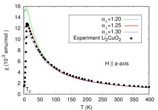
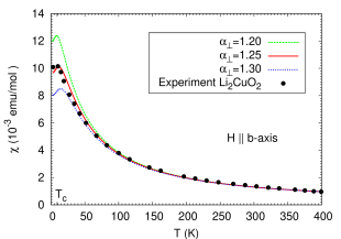
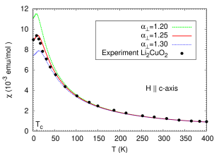
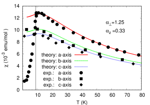
Figure 1: First three panels: theoretical fits for magnetic susceptibility of model (2) to the experimental data for Li₂CuO₂ at $\alpha_{z}=J_{\perp}/J_{z}=0.33$, different values of $\alpha_{\perp}=J_{\perp}/J_{z}$ and for different orientations of magnetic field. The values of $g$-factors, extracted from Curie’s law for different field orientations are: $g_{a}=2.15$, $g_{b}=1.92$, $g_{c}=1.85$. $J_{z}=215K$ and $J^{\prime}=0.33J_{z}$ were taken. Last panel: zoomed view in the vicinity of the transition temperature $T_{c}$ of the experimental data and theoretical curves for all three orientations of magnetic field.

4 Conclusions

In the present manuscript, by using TMRG, we have investigated the possibility to improve the theoretical description of magnetic susceptibility in the edge-sharing cuprate material Li₂CuO₂ upon introduction of a small anisotropy in the NN channel. The main effect of the NN anisotropy at fixed $J_{z}$ appears to be a change in the height of the susceptibility maximum at intermediate temperatures. Namely, the increase of anisotropy $\alpha_{\perp}$ suppresses the maximum, while the decrease of $\alpha_{\perp}$ has the opposite effect. Within the whole range of possible values of $\alpha_{z}$, known from the literature, we found that $\alpha_{z}=0.33$ together with the anisotropy $\alpha_{\perp}=1.25$ best describe the experimental susceptibility data in terms of the model (2). We believe that taking into account the inter-chain coupling along $a-$axis would further improve our description for the corresponding susceptibility at $T<T_{c}$ and such work is currently in progress. The numerical calculations reported in the present article were done in part on CINECA CLX cluster (project No. $954$) and on the CASPUR cluster (project No. $315/09$).

References

References

- [1] Kamieniarz G, Bielinski M, Szukowski G, Szymczak R, Dyeyev S and Renard J P 2002 Comp. Phys. Comm. 147 716 – 719
- [2] Baran M, Jedrzejczak A, Szymczak H, Maltsev V, Kamieniarz G, Szukowski G, Loison C, Ormeci A, Drechsler S L and Rosner H 2006 Phys. Stat. Sol. C 3 220–224
- [3] Lu H T, Wang Y J, Qin S and Xiang T 2006 Phys. Rev. B 74 134425 (pages 9)
- [4] Krug von Nidda H A, Svistov L E, Eremin M V, Eremina R M, Loidl A, Kataev V, Validov A, Prokofiev A and Aßmus W 2002 Phys. Rev. B 65 13445
- [5] Ohta H, Yamauchi N, Nanba T, Motokawa M, Kawamata S and Okuda K 1993 J. Phys. Soc. Jpn. 62 785–792
- [6] Plekhanov E, Avella A and Mancini F 2008 Acta Phys. Pol. A 113 429
- [7] Plekhanov E, Avella A and Mancini F 2008 J. Optoelectron. Adv. M. 10 1675
- [8] Avella A, Plekhanov E and Mancini F 2008 Europhys. J. B 66 295
- [9] Plekhanov E, Avella A and Mancini F 2008 preprint cond/mat–0811.2973
- [10] Mizuno Y, Tohyama T, Maekawa S, Osafune T, Motoyama N, Eisaki H and Uchida S 1998 Phys. Rev. B 57 5326–5335
- [11] Xiang T and Wang X Density-Matrix Renormalization: A New Numerical Method in Physics ed Peschel I, Wang X, Kaulke M and Hallberg K (New York: Springer 1999) p 149
-
[12]
see
http://www.caam.rice.edu/software/ARPACK - [13] Maeshima N and Okunishi K 2000 Phys. Rev. B 62 934–939
- [14] de Graaf C, de P R Moreira I, Illas F, Iglesias O and Labarta A 2002 Phys. Rev. B 66 014448
- [15] Malek J, Drechsler S L, Nitzsche U, Rosner H and Eschrig H 2008 Phys. Rev. B 78 060508
- [16] Drechsler S L, Malek J, Nishimoto S, Nitzsche U, Kuzian R, Eschrig H and Rosner H 2009 J. Phys. Conf. Ser. 145 012060
- [17] Sapina F, Rodriguez-Carvajal J, Sanchis M, Ibianez R, Beltran A and Beltran D 1990 Sol. State Comm. 74 779