Evidence for Non-Linear Growth of Structure from an X-ray Selected Cluster Survey using a Novel Joint Analysis of the Chandra and XMM-Newton Archives

Abstract

We present a large X-ray selected serendipitous cluster survey based on a novel joint analysis of archival Chandra and XMM-Newton data. The survey provides enough depth to reach clusters of flux of $\approx 10^{-14}~{}\mbox{ergs}~{}\mbox{cm}^{-2}~{}\mbox{s}^{-1}$ near $z$ $\approx$ 1 and simultaneously a large enough sample to find evidence for the strong evolution of clusters expected from structure formation theory. We detected a total of 723 clusters of which 462 are newly discovered clusters with greater than 6$\sigma$ significance. In addition, we also detect and measure 261 previously-known clusters and groups that can be used to calibrate the survey. The survey exploits a technique which combines the exquisite Chandra imaging quality with the high throughput of the XMM-Newton telescopes using overlapping survey regions. A large fraction of the contamination from AGN point sources is mitigated by using this technique. This results in a higher sensitivity for finding clusters of galaxies with relatively few photons and a large part of our survey has a flux sensitivity between $10^{-14}$ and $10^{-15}~{}\mbox{ergs}~{}\mbox{cm}^{-2}~{}\mbox{s}^{-1}$. The survey covers 41.2 square degrees of overlapping Chandra and XMM-Newton fields and 122.2 square degrees of non-overlapping Chandra data. We measure the log N-log S distribution and fit it with a redshift-dependent model characterized by a luminosity distribution proportional to $e^{-\frac{z}{z_{0}}}$. We find that $z_{0}$ to be in the range 0.7 to 1.3, indicative of rapid cluster evolution, as expected for cosmic structure formation using parameters appropriate to the concordance cosmological model. Confirmation of our cluster detection efficiency through optical follow-up studies currently in progress will help to strengthen this conclusion and eventually allow to use these data to derive tight contraints on cosmological parameters.

1. Introduction

There is a long history of compiling catalogs of nearby galaxy clusters by using optical telescopes (Abell, 1958; Zwicky et al., 1961). The development of focusing X-ray telescopes and the early discovery of X-rays from clusters of galaxies (Byram et al., 1966) provided another sensitive method for finding clusters of galaxies. A number of X-ray catalogues now exist for the brightest clusters. Most of the nearby clusters are known from flux-limited surveys that cover a large fraction of the sky from ROSAT and Einstein down to $10^{-12}~{}\mbox{ergs}~{}\mbox{cm}^{-2}~{}\mbox{s}^{-1}$ (REFLEX, Böhringer et al. 2004; BCS, Ebeling et al. 1998; EMSS, Gioia et al. 1990). These surveys have discovered 100-450 clusters. Deeper surveys that extend to $10^{-14}~{}\mbox{ergs}~{}\mbox{cm}^{-2}~{}\mbox{s}^{-1}$ and therefore probe a larger range of redshifts have found 60-200 clusters serendipitously (160 square deg., Vikhlinin et al. 1998; 400 square deg. Burenin et al. 2007; ROSAT NEP, Gioia et al. 2001, Henry et al. 2006; WARPS, Scharf et al. 1997, Horner et al. 2008). XMM-Newton surveys have found 19 clusters serendipitously (Georgantopoulos et al., 2005) and 12 clusters in the Large Scale Structure Survey (Willis et al., 2005) down to deeper flux levels.

The slope of the log N-log S distribution for clusters is close to -1 down to a flux limit of $\approx 10^{-13}~{}\mbox{ergs}~{}\mbox{cm}^{-2}~{}\mbox{s}^{-1}$ which means that a wide survey with short exposures will approximately detect the same number of clusters as a narrow survey with longer exposures for the same total exposure time. Thus the total number of clusters is simply proportional to the product of a telescope’s etendue (effective area times field of view) times the total survey exposure time divided by the minimum number of photons that one can reliably use to identify a cluster unambiguously. A large number of the previous surveys used ROSAT which has an area of 200 cm² and a field of view of 3 square degrees. The fields of view of Chandra (0.1 square degrees) and XMM-Newton (0.2 square degrees) are not particularly high, but the effective area of Chandra (400 cm² at 1 keV) and especially XMM-Newton (2000 cm² at 1 keV) are high. XMM-Newton, in particular, has an etendue comparable to ROSAT. One difficulty with using XMM-Newton to perform cluster surveys compared to ROSAT is that the large area and smaller field of view will collect on average more distant groups of galaxies, with smaller angular size, because the survey will be deeper rather than wider for the same exposure time. The fact that the clusters have smaller angular size means that it is harder to determine the difference between a cluster or group and a point source. On the other hand, Chandra has a exquisitely sharp point-spread function (PSF) that distiguishes AGN point sources from clusters at all redshifts across its entire field of view. Therefore, by implementing an analysis method which combines the Chandra PSF with the XMM-Newton throughput, we demonstrate that we can produce a large sensitive X-ray cluster survey.

Recently, a number of independent astronomical methods have converged on a standard cosmological model, which indicates the presence of a poorly understood dark energy component. An extensive search for new galaxy clusters will provide new constraints on cosmological models. In general, the abundance and distribution of clusters of galaxies in the Universe provides precision and complementary cosmological constraints to other methods (Eke et al., 1996). In particular, the measurements are most sensitive to $\sigma_{8}\Omega_{m}$, where $\sigma_{8}$ is the normalization of the matter power spectrum on 8 Mpc scales and $\Omega_{m}$ is the matter density. A large enough sample at a range of redshifts can constrain $w$, the equation of state parameter for dark energy (e.g., Haiman et al. 2001, Wang et al. 2004). The distribution of clusters as a function of mass and the spatial power spectrum constrains cosmological parameters as well.

The content of this initial paper principally concerns the exposition of the new approach for detecting a large sample of X-ray clusters based on a combined analysis of the all useful data in the full Chandra and XMM-Newton archives. We have discovered a new unbiased sample of 462 clusters that reaches the most sensitive flux limit achieved to date ( $10^{-14}~{}\mbox{ergs}~{}\mbox{cm}^{-2}~{}\mbox{s}^{-1}$). We summarize the cosmological implications of this new information with an initial limited approach that assumes the concordance model of the universe is correct and compares the measured Log N-Log S curve of the new X-ray cluster sample with what would be expected in a concordance Universe. The limited scope of this approach precludes a full analysis of the consistency of these new data and the concordance model. We do confirm approximate consistency with the concordance model in two independent ways. First we show that the rapid deviation of the Log N-Log S curve for fluxes less than ( $10^{-13}~{}\mbox{ergs}~{}\mbox{cm}^{-2}~{}\mbox{s}^{-1}$) for a universe without evolution of the density of clusters is consistent with an expected exponential decrease in cluster density for clusters near z $\approx$ 1 and beyond. This result approximately matches the expected density for clusters of mass range expected at a distance of z $\approx$ 1 (see figure 15). Secondly, assuming a concordance model, we compute the expected Log N-Log S curve and find approximate agreement with the newly measured Log N-Log S curve (see figure 16). The detailed explanation of these two comparisons assuming a concordance model appears later in this paper. A full analysis beyond approximate consistency with the concordance model is beyond the scope of this initial paper. In particular, we must improve estimates of several possible systematic errors including the volume of the surveyed region in three dimensions, the exact detection threshold near the flux limit, the re-calibration of the temperature, size, luminosity and mass relations of X-ray selected clusters. We present the log N-log S of the unbiased sample of 462 new clusters without redshift measurements because redshifts (and thus luminosities) are not needed for this initial simple analysis. Future work will address the full cosmological implications of these measurements beyond just the Log N-log S curve for clusters.

2. Basic Methodology

X-ray observations that have both XMM-Newton and Chandra data for the same piece of the sky have the advantage that they can use both the Chandra PSF and the XMM-Newton throughput. For example, finding three photons within one or two arcseconds of each other in a 5 ks Chandra exposure can umambiguously identify an AGN. The probability of background fluctuation or a diffuse source creating that situation is negligible. The number of photons required to determine a point source in XMM-Newton is much higher.

On the other hand, XMM-Newton has $\sim$5 times the effective area and twice the field of view of the Chandra telescope. So over both missions’ lifetimes XMM-Newton has collected 10 times as many photons as Chandra from clusters. Therefore, by simply using Chandra data to find the positions of AGNs, we can subtract photons from the XMM-Newton data and select clusters with as few as 10 to 15 photons. We therefore have a sensitivity several times higher than if we used XMM-Newton data alone. It may be possible to use the full XMM-Newton dataset after calibrating the AGN contribution precisely. The major challenge is to learn how to combine and calibrate all the data and correct for the non-uniformity of the survey. New analysis techniques are required, since the exposures are very deep and contain many smaller clusters at high redshift.

3. Cluster Selection Procedure

Following we describe the basic data processing, image reconstruction, point source removal procedure, and source detection and selection methods.

3.1. Basic Data Processing

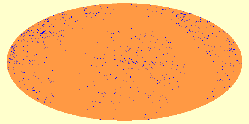
Figure 1.— A map of the survey in equatorial coordinates. The blue regions mark areas where there is either Chandra data or overlapping Chandra and XMM-Newton data. Approximately 0.4% of the sky is covered by this survey. Notably absent is the galactic plane data. The largest contiguous patch in the upper left is the Bootes Chandra survey.

To start this project, we first scanned the XMM-Newton archive for any fields that could potentially overlap with Chandra fields for all data in either archive as of September 2006. Using these fields we can combine the advantages of the Chandra PSF and the XMM-Newton throughput in the following method. A remarkably large fraction (nearly half) of the observations overlap with Chandra observations in at least some part of their field of view. This project clearly benefits from the fact that X-ray observers tend to choose similar targets with both observatories. We downloaded 1201 XMM-Newton fields that overlapped with the the 2706 Chandra ACIS-S or ACIS-I fields. We excluded fields within 10 degrees of the Galactic plane or within 5 degrees of the SMC and LMC. We also included fields that have only Chandra data, since although they will not benefit from the XMM-Newton throughput they can be used to augment the survey with more data with high PSF quality. The positions of the observations are shown in Figure 1. The survey contains approximately 122.2 square deg. of Chandra-alone data with an average exposure of 44 ks and 41.2 square deg. of overlapping XMM-Newton and Chandra data with an equivalent Chandra exposure of 166 ks. Thus, the Chandra-alone data contains about 44% of the cluster candidates and the overlapping survey will contain about 56% because of the relative effective etendues of each sub-survey. A total of 54 Ms of Chandra data and 7 Ms of XMM-Newton data were used.

We used the Chandra level 2 events and applied the standard destreak processing tool. We processed all the XMM-Newton data using the SAS pipeline. The Chandra photon events were selected to have corrected energy (PI) between 0.5 and 7 keV, have no bad data quality flag, and have event pattern less than or equal to 4. The XMM-Newton photon events were selected to have corrected energy (PI) between 0.5 and 7 keV and an event grade of 0, 3, or 4. Background flares were removed from all the 3907 datasets by first binning the events in 100 second time bins. We then iteratively removed 100 second intervals which have the highest count rate until the signal squared (proportional to the number of time bins) divided by the noise (proportional to the total counts) was maximized. This procedure optimally removed the variable component of the background (or a bright flaring AGN). We also removed observations with effective exposures (in ks) divided by the count rate greater than 0.2. This removed extremely short exposures that almost entirely contain background flares.

3.2. Image Reconstruction

We scanned the entire sky and identified all photons from any of the datasets that could have originated in a given grid cell of size 1 square degree. On average there are usually about 2 different observations from either telescope that overlap with a given field position. Within each 1 square degree we only include cluster candidates in the catalog if they fall within the central 0.5 degree by 0.5 degree box, but we analyzed the entire set of photons in the box through the procedure we describe below. The 1 degree square regions were chosen, however, so that they overlapped by 0.5 degrees, leaving no residual binning artifacts.

We only included events from the Chandra data that were within 15 arcminutes of the center of the field of view. This was necessary because the size of the PSF increases significantly at larger angles, but still a large fraction of the data were included. This angle cut also means that some ACIS-S data was included with ACIS-I pointed observations and some ACIS-I data were included with ACIS-S pointed observations. For some particularly deep observations with long exposures, we only included a randomly chosen set of $10^{7}$ photons and then scaled the measurements accordingly, since some of the algorithms we employ below have run times proportional to the number of photons squared. This was rare and only occurs for less than $1\%$ of the datasets.

For every arcminute of the sky, we computed the effective exposure times telescope area (having units $\mbox{cm}^{2}~{}\mbox{s}$) including the effects of telescope vignetting. To do this, we assume that the ratio of effective areas of the ACIS-S, EPIC-PN, and EPIC-MOS were, respectively, 1.4, 4.8, and 1.6 times the ACIS-I area and then we scaled all results of the effective area exposure map to ACIS-I. In reality, the relative area depends on the area of the source, but the values we found were an empirically best averages over all sources and background. Similarly, for the vignetting profile, we assumed a Lorentzian profile of the form $1/(1+(\theta/\theta_{0})^{2})$ where $\theta_{0}$ is 15 arcminutes for XMM-Newton and 25 arcminutes for Chandra. This roughly matched the average energy dependence of the vignetting.

We then removed XMM-Newton photons and set the XMM-Newton exposure-area to zero where there were no Chandra data in either that location in the 1 arcminute exposure-area map or in the adjacent 4 squares in the 1 arcminute exposure-area map. This then conservatively removed any edge effects, and we are left with XMM-Newton events only where there is a complete set of Chandra events. A sample from the Lynx field is shown in Figure 2 after this step where there is a deep exposure with both Chandra and XMM-Newton. After this calculation, we have an estimate of the exposure-area for every square arcminute of the entire sky. For each arcminute of the sky, we also computed the distance to the aimpoint of any exposure for both Chandra and XMM-Newton exposures, in order to compare our candidate sources with an estimate of the PSF size. We also estimated the average count rate for each square degree of the sky for background estimation.

3.3. Point Source Removal

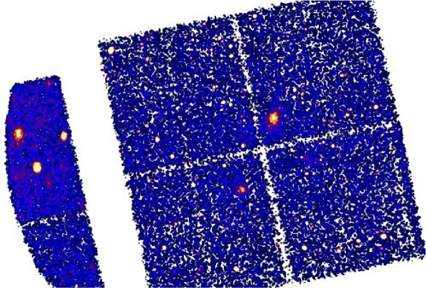
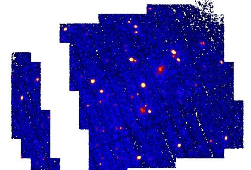
Figure 2.— A Chandra (left) and XMM-Newton (right) exposure of the Lynx field after the non-overlapping XMM-Newton data has been removed. The Chandra field is mostly an ACIS-I pointing and a small piece of the ACIS-S array on the left. This is an example of a deep exposure in the survey with both XMM-Newton and Chandra data. This pixel scale is 5 arcseconds, and the brightest regions correspond to roughly 100 counts per pixel.

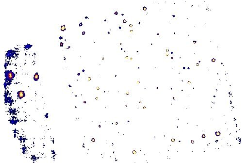
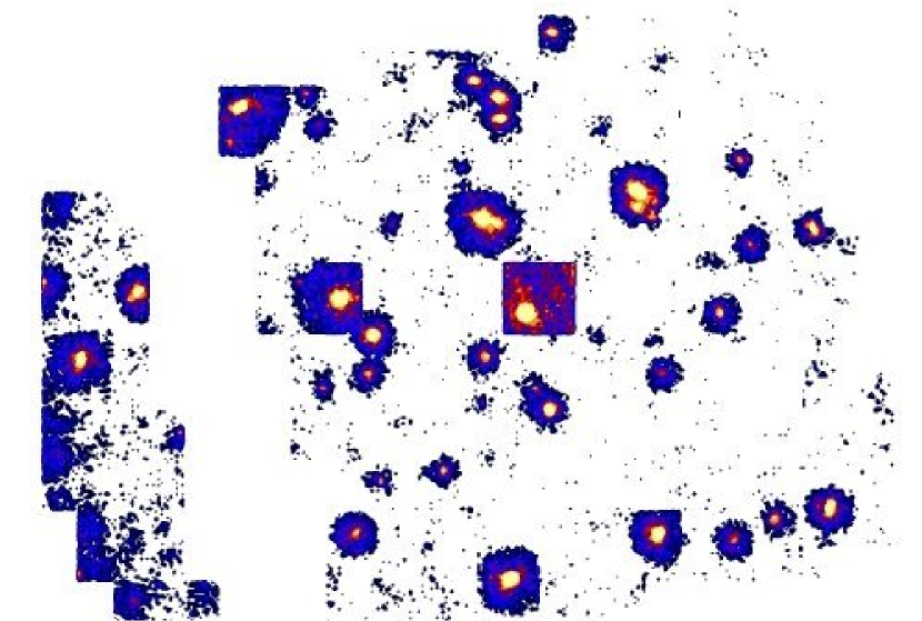
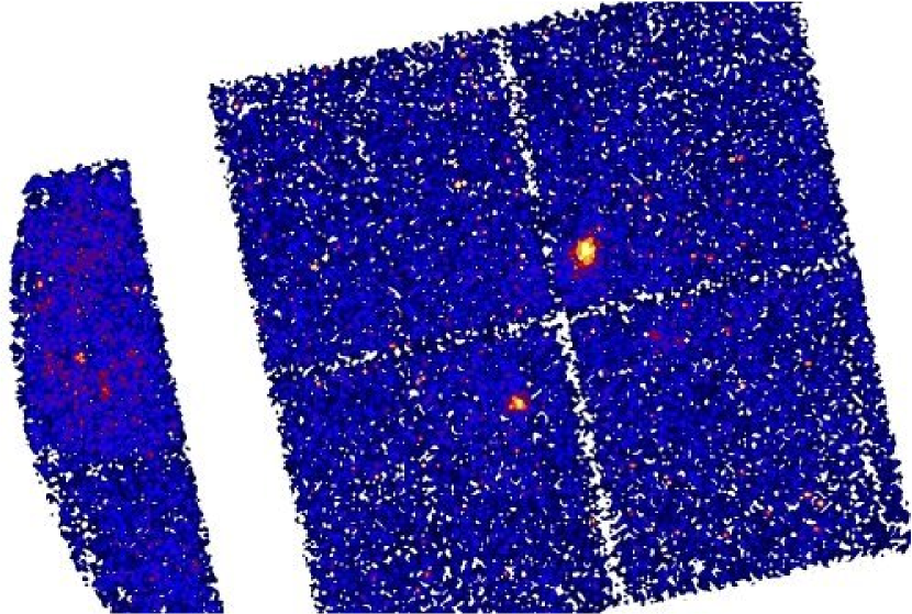
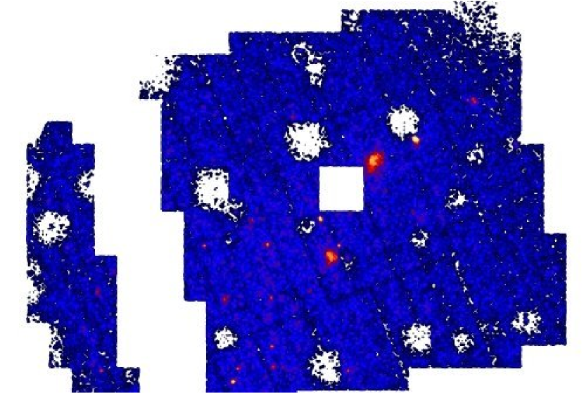
Figure 3.— The upper left panel shows the AGN photons removed from the Chandra data using the method described in the text. The lower left panel contains the cluster candidate emission and background events. The upper right panel shows the corresponding XMM-Newton photons that were subtracted because they were at close to the same position as the Chandra data. The lower right panel shows the XMM-Newton photons after subtracted. The subtraction is not perfect, since the AGN sources vary and the method may over or undersubtract some AGN. However, it is clear most of the AGN emission complicating the source finding in the right in Figure 2 has been removed.

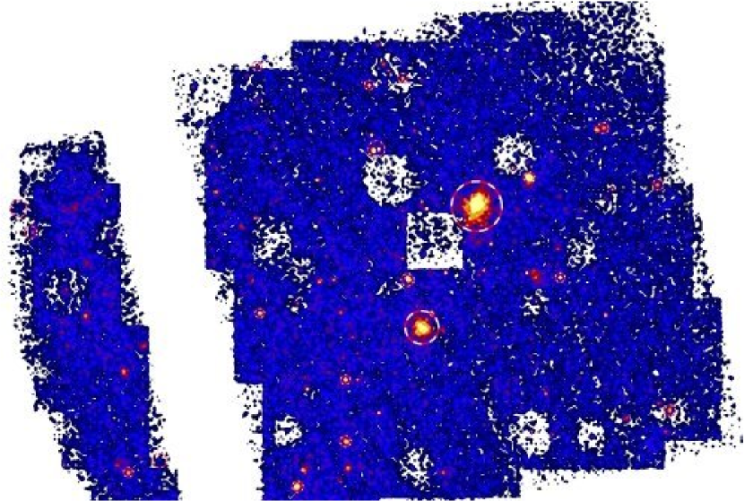
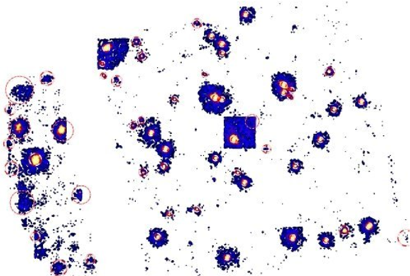
Figure 4.— The cluster candidate and background photons obtained by adding the left images above is shown on the left. Similarly, the co-added AGN emission is shown on the right. The cluster and AGN candidates are then found on these maps using the wavelet method described in the text. The candidates are circled with a size proportional to the size determined from the wavelet methods. The thicker circles correspond to those that satisfy all remaining data cuts. In this case, the two prominent clusters near the center are selected.

Figure 5.— The source flux of the simulated clusters compared to the measured flux using the source detection algorithm as described in the text. Each point represents a different simulated cluster with a different background level (diamonds=$10^{-6}$, squares=$10^{-4}$, triangles=$10^{-2}$, x sign=$10^{0}$, and plus sign=$10^{2}$ counts per pixel). The source flux is the number of photons we put in image, where as the measured flux is the source counts estimated by the wavelet method. The source size is the core radius of the beta model and the measured size is the most significant size of the wavelet method times the correction factor.

Using the Chandra photons alone we located the point sources by finding photons where the number of neighbors within the local PSF size exceeded the number of photons within twice the local PSF size by two sigma. We only searched through a subset of photons in the relevant 1 by 1 arcminute block or the adjacent 1 by 1 arcminute block. This improved the computation efficiency of the algorithm. The local PSF size was estimated to be $(3+20(\frac{\theta}{\theta_{1}})^{2})$ arcseconds where $\theta_{1}$ is 15 arcminutes. Photons which satisfied this condition held were tagged as candidate “AGN” photons. We also randomly untagged a fraction of these photons in proportion to the relative count rate of photons with a local PSF size to twice a local PSF size. This allowed us to fill back in some photons which may be due to background. All Chandra photons were then tagged as either “AGN” photons like those in the top left panel in Figure 3 or “Cluster+Background” photons like those in the lower left panel in Figure 3.

Then for each Chandra photon we removed a set of the nearest XMM-Newton photons (when there are any) given by the ratio of the exposure-area maps we computed earlier. The nearest XMM-Newton photon was found by computing,

$$\sqrt{\frac{\Delta x^{2}+\Delta y^{2}}{(10^{\prime\prime})^{2}}+\frac{\Delta e^{2}}{(150\mbox{eV}\sqrt{e_{keV}})^{2}}}$$

.

where $\Delta x$ and $\Delta y$ are the difference in spatial coordinates, $\Delta e$ is the difference in measured photon energy (in eV), and $e_{keV}$ is the photon energy. Thus, the selected photons were chosen to have a similar position and have similar energy. If the ratio of exposure-area maps was not an integer, we chose random numbers appropriately to decide whether to add extra photons to obtain the proper normalization. We also did not use XMM-Newton photons outside of a 2 by 2 arcminute block as with the previous step for computational efficiency. This method then selected the XMM-Newton AGN photons even if the XMM-Newton PSF was large and if it was difficult to determine if the source was a cluster or AGN from the XMM-Newton data alone. We then have two sets of photons for the XMM-Newton data as well: those that are removed are composed primarily of AGN photons (top right in Figure 3), and those that have not been removed that are either from clusters or background (bottom right in Figure 3). The method is imperfect when the AGN flux varies significantly between observations and due to noise, but we can estimate this by comparing the two maps. If we subtracted a lot of “AGN” photons at a particular location and we found a source in the subtracted map then this was likely due to a subtraction problem. This is described in more detail in the next section.

3.4. Source Detection and Selection

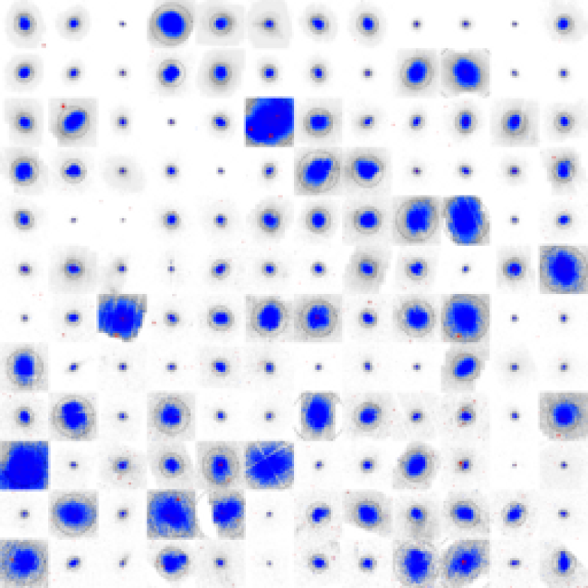
Figure 6.— The full catalog of cluster candidates (continued on next pages). The subtracted AGN emission is shown in red, whereas the cluster emission is shown in blue. The dotted circle represents twice the fitted wavelet size of the source detection algorithm.

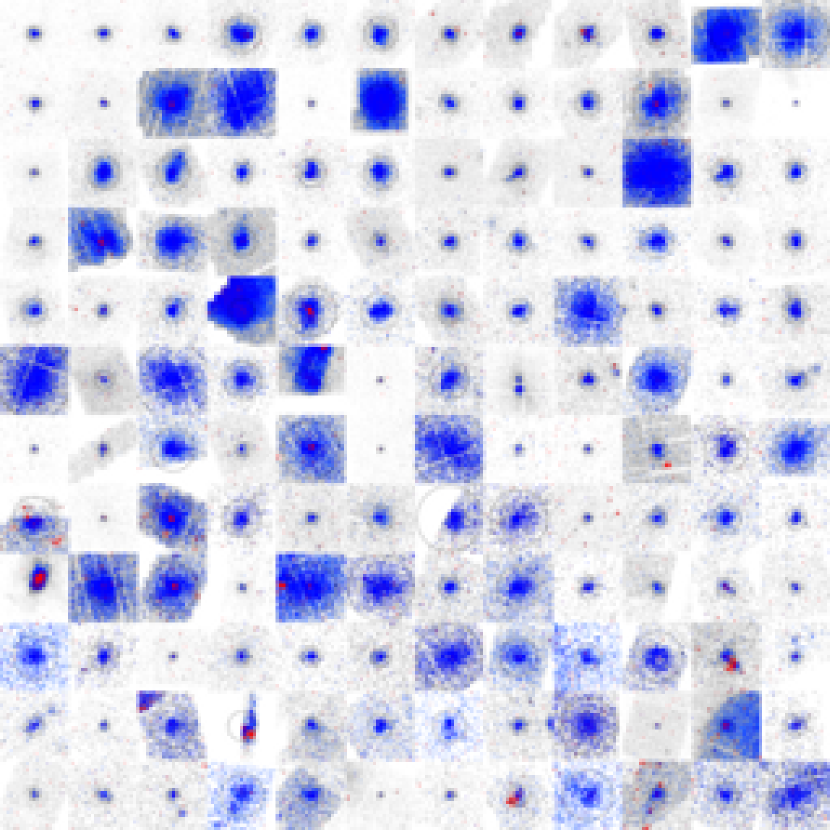
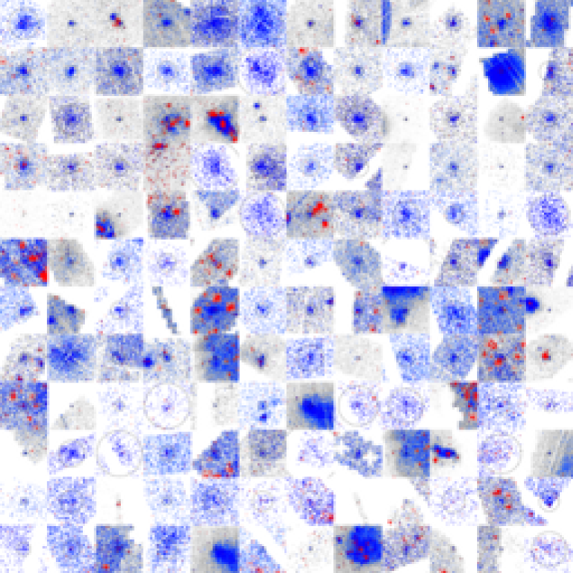
Figure 7.— The full catalog of cluster candidates (continued). The subtracted AGN emission is shown in red, whereas the cluster emission is shown in blue.

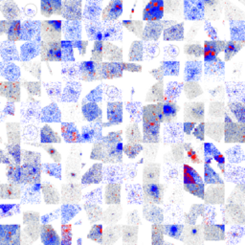
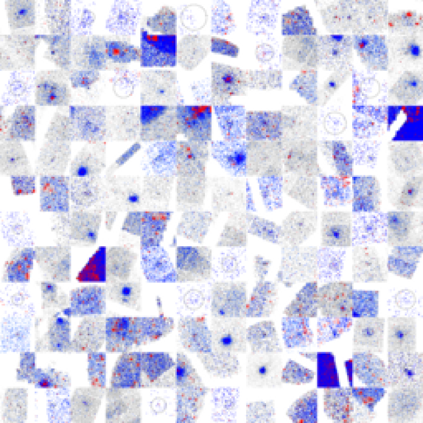
Figure 8.— The full catalog of cluster candidates (continued). The subtracted AGN emission is shown in red, whereas the cluster emission is shown in blue.

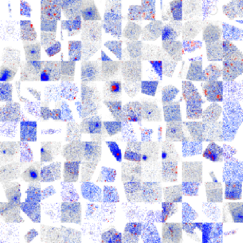
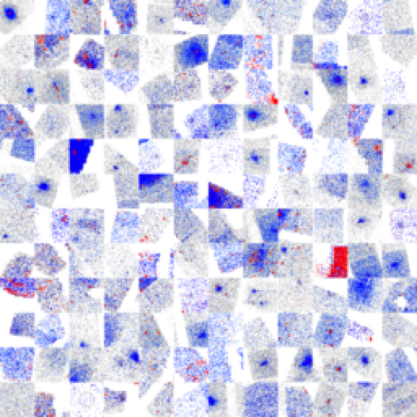
Figure 9.— The full catalog of cluster candidates (continued). The subtracted AGN emission is shown in red, whereas the cluster emission is shown in blue.

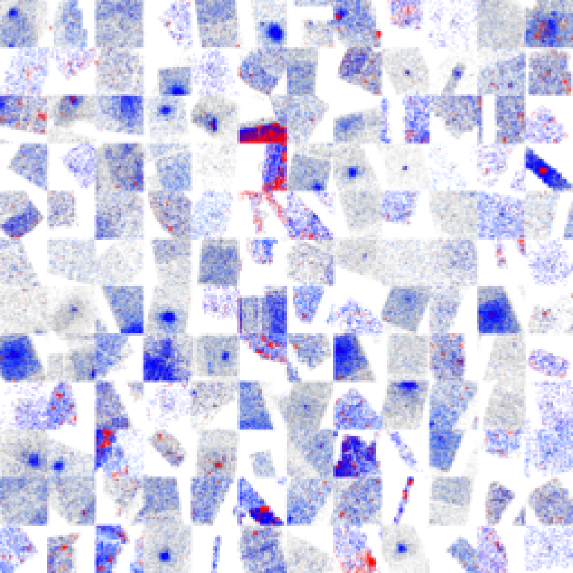
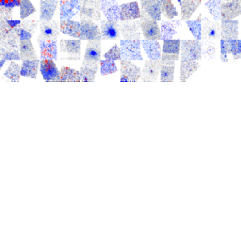
Figure 10.— The full catalog of cluster candidates (continued). The subtracted AGN emission is shown in red, whereas the cluster emission is shown in blue.

Next, we constructed the combined maps by adding the XMM-Newton and Chandra maps for AGN photons and clusters and background photons, respectively as shown in Figure 4. We only included photons from 0.5 to 2 keV, since now we wanted to maximize our sensitivity to finding new clusters and most of the cluster emission occurs in the soft band. We binned the photons into a 5 arcsecond grid and then find sources using a wavelet method which is a modified form of that described by Vikhlinin 1998. To do this, we computed functions of the following form:

$$g(x_{0},y_{0},\sigma)=\frac{1}{2\pi\sigma^{2}}\int f(x,y)e^{-\frac{(x-x_{0})^{2}+(y-y_{0})^{2}}{2\sigma^{2}}}$$

where $g$ is a gaussian convolution of the map $f$ with scale $\sigma$. These convolutions can be calculated most efficiently in Fourier space. An estimate of the number of photons of a given source at position $(x_{0},y_{0})$ of size $\sigma$ is given by

$$c(x,y)=\left(\frac{g_{sc}(x_{0},y_{0},\sigma)}{g_{ea}(x_{0},y_{0},\sigma)}-\frac{g_{sc}(x_{0},y_{0},2\sigma)}{g_{ea}(x_{0},y_{0},2\sigma)}\right)$$

where the $g_{sc}$ is the integral above using the soft band counts and $g_{ea}$ is the integral using the exposure-area function. When the area-exposure map is constant this function will be equivalent to the normal spherical top-hat function used in wavelet applications. We stepped through every pixel of the map using source sizes from 1 to 32 pixels in step size of $log_{2}(\mbox{radius})$ of 0.2. We also estimate the hard band counts (2.0 to 7.0 keV) and the AGN soft band counts at the same position. The background rate was estimated locally by convolving a gaussian with $\sigma$ of 480 arcseconds (3 times the largest source we allow). We found that the detection significance of a source could then be estimated by the formula

$$\mbox{significance}=\frac{c}{n}/\sqrt{\frac{b}{n}}-4(b\sigma^{2})^{-0.4}$$

.

where $c$ is the counts function defined in the previous equation, $b$ is the background function using the previous equation with width of 480 arcseconds, and $n$ is a normalizing factor $\frac{9}{80\pi\sigma^{2}}$. We determined this function by performing Monte Carlo simulations of pure poisson noise. The first term dominates for high count rates and follows the gaussian form, and the second term corrects for the fact that at low count rates the distribution is non-gaussian. The detection significance, therefore, depends both on the number of photons in the source and the source size. We also found it necessary to calculate the signal to noise as well as the source significance (signal divided by the square root of noise), because there were highly significant large sources that had low signal to noise. We then have a set of candidate sources at various positions and sizes. We only select sources with significances greater than 6 sigma and signal to noise greater than one. These limits were chosen so that we at most have one spurious source in the entire survey due to background fluctuation and do not include low signal to noise sources that may be due to non-statistical background calibration errors.

At this point, the candidate sources could overlap and be at adjacent locations because they all have enough detection significance. To select a unique set of sources, we simply remove any candidate source that is within 3 source radii from another and has lower significance. The source radius is defined as the maximum $\sigma$ of the two sources being compared. We found that this visually results in only one object being detected per actual source quite efficiently.

To test the ability to correctly measure the flux and size of sources, we performed a series of photon Monte Carlo simulations. We first randomly generated between 30 and 10,000 photons representing a cluster using a $\beta$ model. The core radius was randomly chosen between 2 and 10 pixels and $\beta$ was chosen between 0.5 and 0.75. We then chose a background level randomly between $10^{-6}$ and $10^{2}$ counts per pixel having Poisson noise. This simulates the wide range of sources and conditions that we might find. We then used the source finding algorithm on the simulated image and found that the source flux was accurately recovered and the source size was accurately measured even in the presence of the different background conditions. This is shown in Figure 5. The typical scatter from the true values was $20\%$ and $30\%$ for the source size and flux, respectively. We also note that we recovered 495 out of the 500 sources we simulated. This indicates that our source finding algorithm is fairly robust to a range of background levels and source fluxes.

We then have a large number of cluster candidates. We found it necessary to employ four further selection criteria to remove non-clusters. First, we computed the ratio of the counts in the cluster candidate to the counts in the AGN map. We required this ratio to be greater than 4. Without this requirement, AGN which have increased flux between the Chandra and XMM-Newton exposures will be undersubtracted. This is rare since the variability is typically only about 10$\%$, but there are also many AGN candidates.

We also found it necessary to require that the source size plus three times the measurement error is at least 4 arcseconds larger than the local PSF size,

$$\sqrt{(\mbox{size}+3\sigma_{\mbox{size}})^{2}-(\mbox{PSF})^{2}}\geq 4^{\prime\prime}$$

This is a very conservative cut that removes about 30$\%$ of the potential candidates. Since, we have added three times the source size error, we are only effectively removing candidates that have very little chance of actually being legitimate clusters. We then expect that only a small fraction of this 30$\%$ would be real clusters or groups that are removed accidentally. The local PSF size is estimated by combining quadratically the estimate for the local Chandra PSF given in the previous section with the XMM-Newton PSF in proportion to their exposure area. The XMM-Newton PSF is assumed to be 10 arcseconds across the field of view, since it changes shape but its size does not change dramatically. The size error is determined by simply dividing the size by the square root of the number of counts. Thus, by using the AGN photon subtraction method above we have removed the vast majority of AGN emission but there is some residual background due to AGN variability. Although this limits our ultimate sensitivity, our method is several times more sensitive than just finding sources and estimating the size without the photon subtraction.

We also estimate the ellipticity of the source by calculating the second moment of the counts weighted by a gaussian with width equal to the size of the source. We then require the ellipticity to be less than 0.25. This does not remove any clusters, but removes some spurious sources due to the readout streak.

We also removed cluster candidates where the ratio of counts in the soft band over the counts in the hard band (the spectral softness, $s$) follows the equation,

$$s-3\sigma_{s}^{\frac{1}{2}}\geq 1$$

.

This cut cleanly removes some systematic fluctuations in the background. The softness of the background is defined as exactly 1, since we set the middle our bands to be the median of the energy as described previously. For XMM-Newton this results in energy range of 0.5 to 1.7 keV for the soft band and 1.7 to 7.0 keV for the hard band. For Chandra this results in an energy range of 0.5 to 2.2 keV for the soft band and 2.2 to 7.0 keV for the hard bands. A high temperature, $\sim 8keV$, cluster has a softness near $2.5$, however, and a lower temperature cluster has a much higher spectral softness.

Finally, we found it necessary for some of the final candidates to be removed by human inspection, since they were obvious supernovae remnants, planets, or knots in emission that had survived all of our cluster selection procedures. We utilized a 4 node computing cluster to perform the calculations for this procedure on all the data sets in about a week, and perfected it after many iterations. After all the data selection procedures, we have 1198 cluster candidates as shown in Figure 6. Many of these clusters were known sources and were in fact the targets of the relevant observation. There are 462 clusters that are outside of 4 arcminutes from the central pointing. Later we will argue on the basis of the log N-log S distribution that this is a reliable estimate of the number of new clusters.

After all these cuts we were able to use the AGN in our sample to estimate how many of these objects would survive if they were incorrectly chosen as cluster candidates due to some mistake in the photon removal procedure. We find that 19 AGN would survive these cuts that were more than 4 arcminutes outside the central pointing. Thus, we estimate that the contamination in our survey of false clusters is about 3$\%$. We also need to estimate the efficiency of not removing real clusters. We have, however, performed Monte Carlo simulations that found 99$\%$ of all of our simulated clusters. We note, however, that the cuts we have used above are designed to only remove objects that have completely inconsistent properties of a normal cluster. The one cut to worry about in particular might be the size cut, which could remove some particularly small groups. This cut, however, only removes 30$\%$ of the candidates so even if some of these were real clusters it probably would not be much more than 3 to 5 $\%$. Furthermore, none of the cuts remove any of the brightest 100 already well-known clusters. Thus, we estimate that the efficiency of these candidate cuts is around 95$\%$ and that might roughly cancel with the 3$\%$ estimation for contamination. Both of these estimates can be constrained more rigorously with simulations and optical follow-up.

4. Comparison with previously known clusters

Since we have used archival observations, a significant fraction of our sample will be comprised of previously known clusters that were the targets of their respective observations. In order to compare the cluster candidates with previously known clusters, we used the NASA Extragalactic Database (NED). NED currently contains over 40,000 cluster candidates from over 300 surveys. In order to check our cluster candidates reliably, we deconstructed the NED catalog into the individual cluster catalogs. We then cross-correlated that catalog with itself to select objects within 1 arcminute of each other. A reasonable way to be confident that the cluster candidates are real is to simply require that the object appear in multiple catalogs whether they are X-ray surveys, optical, or any other kind of survey. We found that 261 (out of 1198 that passed our selection cuts) clusters in our survey were previously known. There was also a significant number of sources at the center of the field of view that were nearby galaxies and other extended sources.

5. Log N-Log S Distribution

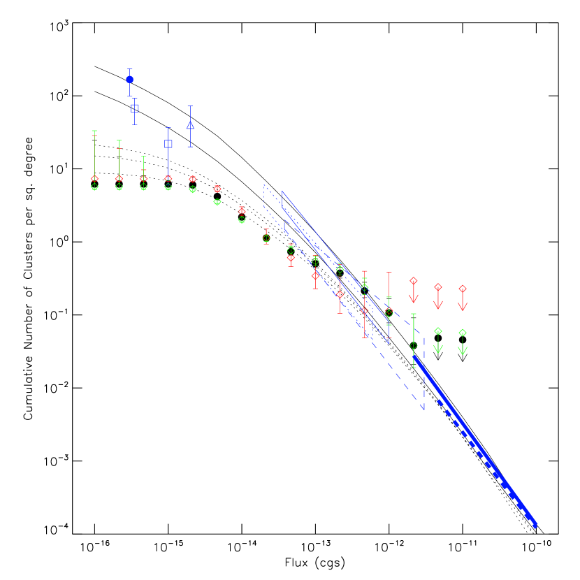
Figure 11.— The log N-log S distribution for all the cluster candidates (black), the XMM-Newton/Chandra overlap candidates (red diamonds), and the Chandra only candidates (green diamonds). The models are (black lines from top to bottom): no evolution with $\alpha=1.7$, $L_{x}^{*min}=2\times 10^{41}~{}\mbox{ergs}~{}\mbox{s}^{-1}$, $\phi^{*}=2.7\times 10^{-7}\mbox{Mpc}^{-3}$, no evolution with $\alpha=1.6$, $L_{x}^{*min}=2\times 10^{42}$, $\phi^{*}=1.8\times 10^{-7}$, and evolution models with $z_{0}=0.7,~{}1.0,~{}1.3$ using the latter set of parameters (see text). The blue lines are those of Bauer 2002 (circle), Giacconi et al. 2002 (square), McCardy et al. 1998 (triangle), Henry et al. 2001 (dashed box), Rosait et al. 1998 (dotted box), Vikhlinin et al. 1998 (solid box), Böhringer et al. 2001 (solid line on right), and Ebeling et al. 1998 (dotted line on right).

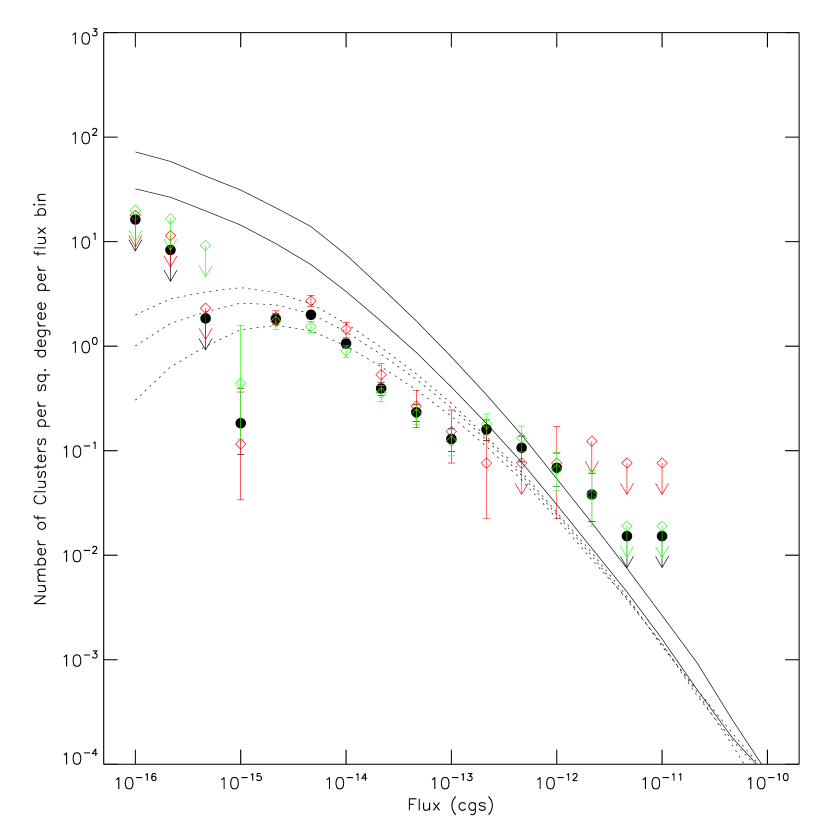
Figure 12.— Identical plot to the previous plot except in differential form.

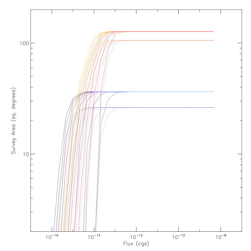
Figure 13.— The survey area in square degrees as a function of flux for different source sizes (4 (left most) to 256 (right most) arcseconds in multiples of 2). The blue curves are the overlap survey and the red curves are the part of the survey where there is only Chandra data. The Chandra-only survey has a larger area, but does not go as deep as the XMM/Chandra overlap survey. The dotted curve shows the area after the 4 arcminute central pointing region is excluded.

Figure 14.— The log N-log S distribution for the cluster candidates showing the effect of the size cut. We plot the same curves as in Figure 11, but we show both a size cut of zero arcseconds (lower curve) and eight arcseconds for the same model parameters as before except we only include $z_{0}=1.0$ for clarity. Clearly, the size cut has very little effect above fluxes of $10^{-14}~{}\mbox{ergs}~{}\mbox{cm}^{-2}~{}\mbox{s}^{-1}$.

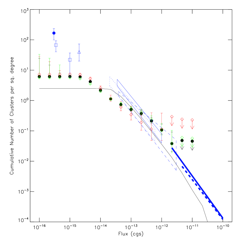
Figure 15.— The expected number density of clusters compared to the present number density. The blue dashed region is the region enclosed by our measured exponential function. The three curves correspond to the number density for cluster of mass of $3\times 10^{13}$, $10^{14}$, and $3\times 10^{14}$ solar masses (from right to left) using the calculation described in the text from structure formation theories for concordance cosmology. The exact shape of the rapid turnover is not important, but these curves demonstrate that structure formation theories predict a similar rapid evolution in the number density close to the observations.

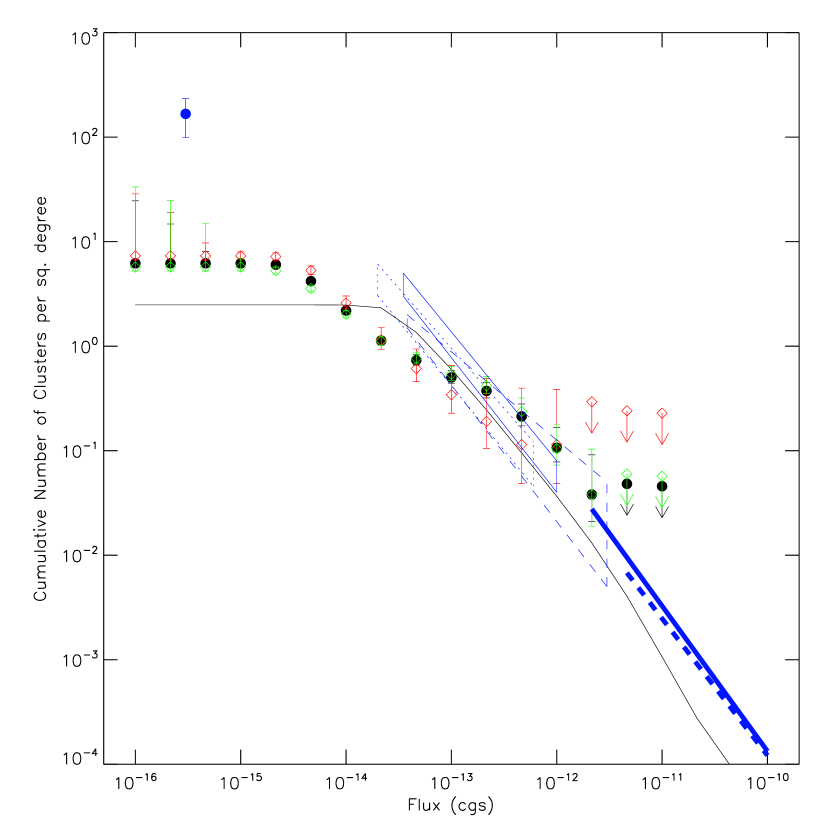
Figure 16.— The log N-log S distribution as before, but using the direct calculation of the distribution from structure formation theory. See the text for further details.

We constructed the log N-log S distribution for the clusters in our sample as shown in Figure 11. We plotted the log N-log S distribution in both the cumulative and differential forms (Figure 12). The conversion from counts to flux was calculated by using WebPIMMS using a column density of $2\times 10^{20}\mbox{cm}^{-2}$, $kT=4keV$, and abundance of 0.4 solar. Although there is obviously variation in our clusters, the variation will be less than our flux bin width and these are expected typical values. The log N-log S distributions are then calculated by adding up the number of sources divided by the area of the survey that source in which that source could have been detected. Since we have a different flux limit for every point in the survey, we had to take this into account. Furthermore, our source detection sensitivity depends on the object’s measured wavelet size. Therefore, we calculated the survey area as a function of flux for each object taking into account our source selection function in Figure 13. For each square arcminute of the survey we calculate the total exposure and multiply that by a given flux. This gives us an estimate of the number of photons that would be produced by a source at that particular place in the sky. Then we see if that would pass both our significance cut described in Section 3.4 and our signal to noise cut for the background at that particular place in the field. Thus, at high source fluxes the survey area is the full survey, but at low source flux it will be lower. We have assumed that our other selection cuts do not remove significant numbers of real clusters and largely remove spurious data artifacts. Our earlier Monte Carlo simulations indicate for a wide range of sources that most of these (99$\%$) are recovered by the source finding algorithm.

We examined the subset of sources located a distance $A$ from the centers of observations in which they were detected, and varied $A$ until the log N-log S distribution convered. This occurs for $A$ $\sim$ 4 arcminutes. We take this as an indication that the application of that cut removes the bias associated with selected pointings at known clusters. We also separated the Log N-Log S points for the overlapping Chandra and XMM-Newton survey (red diamonds) and the Chandra only data (green diamonds ). The difference in these surveys gives us a rough measure of the systematic error, since these are completely different samples.

We modelled the log N-log S distribution using the following method. First to be consistent with previous large angle surveys we adopted the Schechter function as outlined in the review by Rosati, Borgani, & Norman 2002,

$$\frac{dN}{dL_{X}}=\frac{\phi^{*}}{L_{x}^{*}}{\left(\frac{L_{x}}{L_{x}^{*}}\right)}^{-\alpha}e^{\left(-L_{x}/L_{x}^{*}\right)}e^{\left(-L_{x}^{*min}/L_{x}\right)}$$

where we added the last factor to possibly cut off the luminosity on the low luminosity end to account for small groups that will not even emit X-rays even if they obey scaling relations. We used the values of $\alpha=1.7$ (has 15$\%$ scatter in the literature), $L_{x}^{*}=4\times 10^{44}~{}\mbox{ergs}~{}\mbox{s}^{-1}$, $\phi^{*}=2.7\times 10^{-7}\mbox{Mpc}^{-3}$ (has 50$\%$ scatter in the literature) from Rosati, Borgani, & Norman 2002 which summarize the previous work at the high flux end. We also used slightly lower values of $\alpha=1.6$ and $\phi^{*}=1.8\times 10^{-7}\mbox{Mpc}^{-3}$ for a second calculation than the mean values measured in other work but still within the observational uncertainties to be conservative about the measurement of evolution as we discuss below. We then use this luminosity function and the comoving volume element of the Universe for $\Lambda CDM$ ($\Omega_{m}=0.25,\Omega_{\Lambda}=0.75$) to populate the Universe with clusters as a function of redshift. Then, we convert the luminosities of the clusters using the appropriate luminosity distance for the same cosmology. We also predict the fraction of these clusters that would be missed by our size cut by estimating the physical size, $R$ of the cluster following the relation of

$$R=1\mbox{Mpc}{\left(\frac{L_{x}}{10^{46}\mbox{ergs}~{}{s}^{-1}}\right)}^{0.45}$$

.

We determined this relation by looking at the clusters in our sample where we knew the redshift. This physical distance is converted into an angular size using the angular diameter distance for the same cosmologies. This allows us to predict the log N-log S distributions in Figure 11.

We varied $L_{x}^{*min}$ between $2\times 10^{41}~{}\mbox{ergs}~{}\mbox{s}^{-1}$ and $2\times 10^{42}\mbox{ergs}~{}\mbox{s}^{-1}$ which had an minor effect on the curves. A luminosity of $2\times 10^{42}\mbox{ergs}~{}\mbox{s}^{-1}$ would correspond to a object with virial temperature around 400 eV and a luminosity of $2\times 10^{41}~{}\mbox{ergs}~{}\mbox{s}^{-1}$ would correspond with a virial temperature around 100 eV. Even if there are many objects in the Universe with these sizes they would stop emitting significant X-rays somewhere in this range since the flux is located out of the X-ray band in this temperature range.

Similarly, the cosmological parameters used in the calculation of the volume element have a small effect as well. We adopted the concordance values of $\Omega_{m}=0.25$, $\Omega_{\Lambda}=0.75$, and $H_{0}=72\mbox{km}\mbox{s}^{-1}\mbox{Mpc}^{-1}$. If we assume no evolution in this luminosity function then the data are completely inconsistent with the model using the nominal set of parameters for $\phi^{*}$, $L_{x}^{*min}$, and $\alpha$ as well as a conservative set of values for these parameters as shown in Figure 11. On the other hand, if we modify $\phi^{*}$ by a factor of $(1+z)^{q}$ we can match the data only if q is greater than -2. This demonstrates that we have measured the onset of cluster formation and have observed the dearth of clusters at high redshift. Since the $1+z$ formulation shows rapid evolution, we have also simply tried to represent this rapid evolution as a $e^{-\frac{z}{z_{0}}}$ instead. In Figure 11, we plot values of $z_{0}$ of 0.7,1.0, and 1.3 along with the no evolution case. Given the parameters of the model we have used, the data points towards rapid evolution at relatively low redshift of z=0.7 to 1.3. The exact value may depend somewhat on our choice of parameters for the normalization and slope of the luminosity function. It also might be affected by unaccounted for inefficiencies of the survey which could reduce the number of observed clusters by 10 to 20%. Note, however, that the size cut only mildly reduces the number of clusters and that cut would have to be falsely removing clusters as large as 20 arcseconds instead of 4 arcseconds to explain the evolution. To demonstrate this, we show the effect of a zero arcsecond and eight arcsecond cut in Figure 13. Generally, there is little effect below a flux of $10^{-14}~{}\mbox{ergs}~{}\mbox{cm}^{-2}~{}\mbox{s}^{-1}$. For that reason, it is very likely that the observed deficit at low fluxes is due to an actual absence of clusters at high redshift. Note also that our exponential function describes the number density of clusters and not the absolute number of clusters which will peak at higher redshifts.

This rapid evolution is generically predicted in models of structure formation with a non-negligible amount of matter in the Universe. Structure formation models predict a decrease in both the normalization of the cluster mass function at high redshift as well as a change in shape of the function (Jenkins et al., 2001). Furthermore, if there is significant cluster evolution as we have argued, then the parameterization of evolution in terms of $(1+z)^{q}$ or $e^{-\frac{z}{z_{0}}}$ is an oversimplification. In Figure 14, we plot the range of exponential functions derived to match the log N-log S distribution. We then overlay the expected number density of clusters combining the Jenkins et al. 2001 theory with the power spectrum of Eisenstein & Hu 1999 in an identical calculation to that of Haiman et al. 2001 for three different mass of clusters. We use the concordance parameters above and also set $\sigma_{8}=0.75$, $\Omega_{b}=0.04$, $w=-1$, and $n_{s}=1.0$. The agreement clearly demonstrates that the rapid evolution that we have measured is similar to what is expected for reasonable cluster masses. Future detailed measurements and modelling when masses and redshifts can be estimated may measure the exact nature of the cluster evolution.

The structure formation model predicts an evolution that varies as a function of mass, so we can predict the log N-log S distribution directly as an additional check. We must make the additional assumption of a mass-luminosity relation and assume that the theoretical mass function agrees well with the local luminosity function. We adopt the mass-luminosity relation of Stanek et al. 2006 where $L_{44}=3.8\left(\frac{M}{10^{1}5h^{-1}}\right)^{1.59}$. We ignored any redshift dependence of the relation to be conservative, since the change in the relation would make the evolution more significant. We also assume that simulated clusters with calculated luminosities below $2\times 10^{42}~{}\mbox{ergs}~{}\mbox{s}^{-1}$ are suppressed by the same exponential function as before. The direct log N-log S calculation is shown in Figure 15, and agrees quite well given the uncertainties in our mass calibration.

Our results are generally consistent with intermediate flux ROSAT surveys at $10^{-13}\mbox{ergs}~{}\mbox{cm}^{2}~{}\mbox{s}^{-1}$ as measured in Henry et al. 2001, Rosait et al. 1998 and Vikhlinin et al. 1998. Near a flux of $10^{-14}~{}\mbox{ergs}~{}\mbox{cm}^{2}~{}\mbox{s}^{-1}$ our results deviate somewhat particularly with those of Vikhlinin et al. 1998 and are closest to those of Henry et al. 2001. A combination of some non-cluster contamination and an underestimate of the survey sensitivity could explain these discrepancies. Considering the error ranges, however, these measurements could still be consistent with some mild cluster evolution. Our results are complementary to those at high fluxes, e.g. Böhringer et al. 2001, and we have fixed our theoretical model consistent with those results.

Our results are also broadly consistent with the recent work of Vikhlinin where cluster masses have been estimated for a sample of 36 clusters Vikhlinin et al. 1998. In this work, he demonstrated that a lower redshift sample ($z\sim 0.1$) had a different and lower normalization mass function than the cluster at higher redshift $z\sim 0.5$. The results were consistent with the concordance structure formation model discussed above. In a later work, Vikhlinin measured the equation of state parameter for dark energy to 10$\%$ Vikhlinin et al. 2008. Since our sample is larger and deeper, it might be possible to measure the equation of state parameter to 2$\%$ in a different mass and redshift regime.

Our results are inconsistent, however, with the log N-log S distribution determined using the Chandra deep field (Bauer, 2002). This was determined by using 130 square arcminutes and finding six candidates clusters in that survey that suggested there was no evolution in the cluster luminosity function. These objects, however, have signal to noise less than 1 (table 1, column 6 of their paper), so would not survive our signal to noise cut. If we remove our signal to noise cut we find 3 out of the six objects. If only two or three are clusters, then we would be consistent with this measurement. Similarly, both McCardy et al. 1998 and Giacconi et al. 2002 found clusters in deep and narrow surveys. Giacconi et al. 2002 do not make a claim about cluster number density. If we convert their data to log N-log S as in Rosati, Borgani, & Norman 2002, then they are consistent with our measurements at $10^{-15}~{}\mbox{ergs}~{}\mbox{s}^{-1}$ but inconsistent at lower fluxes. Giacconi et al. 2002 argue, however, that many of these sources could be contaminated by hard X-ray emission from AGN.

Our results are consistent with previous measurements of the evolution of the luminosity functions where the redshifts were known in the Rosat Deep Cluster Survey and the Einstein Medium Sensitivity Surveys (Gioia et al. 1990 and see Figure 9 in Rosati, Borgani, & Norman 2002), although the interpretation is somewhat different. There the authors considered both an evolution in the normalization and the value of $L_{X}^{*}$ (in their notation the parameters are A and B). In our case, the evolution factor, $q$, is equivalent to $A+B$. The previous results have constrained the value of $A+B$ to be approximately equal to $-3$, which is also completely consistent with our result. The other authors have argued, however, that the data are more consistent with mostly a non-zero value of $B$, which we cannot distinguish from the flux distribution alone. In addition, our sample is much deeper and it is likely that the Schechter formulation is not even correct to such a large range in redshifts. In any case, negative evolution in the clusters x-ray luminosity function and the emergence of clusters in the Universe has been clearly observed. Additional detailed photon Monte Carlo simulations like those we have proposed above as well as optical follow-up to remove spurious sources are needed to verify the efficiency and contamination we have claimed in the log N-log S calculation. However, the large deviation of the Log N-Log S curve at $10^{-14}~{}\mbox{ergs}~{}\mbox{cm}^{-2}~{}\mbox{s}^{-1}$ compared to the future model is beyond any reasonable expected systematic error.

6. Future Work

There are several research areas that can be pursued in the future with this cluster sample. First, the efficiency of the survey can be carefully calculated by futher Monte Carlo simulations. Second, the bias of the survey can be more accurately estimated by performing a blind survey on a modest field. Third, the redshifts of the new clusters can be measured by optical and IR follow-up including cluster verification. Fourth, the cluster abundance can be measured by combining the efficiency calculation and the redshifts. Fifth, the X-ray estimated cluster masses can be compared to weak lensing measurements for at least some of the clusters. Then by assigning these clusters to a given mass and redshift, the structure formation theory can be tested in great detail. Finally, the XMM-Newton and Chandra archive continues to accumulate more data, so a much larger survey can be performed in the future. Some portion of this additional work is necessary prior to a robust estimate systematic errors of cosmological parameters.

References

- Abell (1958) Abell, G. O. 1958, ApJS, 3, 211.
- Bauer (2002) Bauer et al. 2002, ApJ, 123, 1163.
- Böhringer et al. (2004) Böhringer, H., et al. 2004, A&A, 425, 367
- Böhringer et al. (2001) Böhringer, H., et al. 2001, å369, 826.
- Byram et al. (1966) Byram, E. T., Chubb, T. A., & Friedman, H. 1966, Science, 152, 66
- Burenin et al. (2007) Buernin et al. 2007, ApJS172, 561.
- Ebeling et al. (1998) Ebeling, H., Edge, A. C., Bohringer, H., Allen, S. W., Crawford, C. S., Fabian, A. C., Voges, W., & Huchra, J. P. 1998, MNRAS, 301, 881
- Eisenstein & Hu (1999) Eisenstein, D. & Hu, W. 1999, ApJ411, 5
- Eke et al. (1996) Eke, V. R., Cole, S., & Frenk, C. S. 1996, MNRAS, 282, 263
- Georgantopoulos et al. (2005) Georgantopoulos, I., Georgakakis, A., & Koulouridis, E. 2005, MNRAS, 360, 782
- Giacconi et al. (2002) Giacconi et al. 2002, ApJS139, 369.
- Gioia et al. (2001) Gioia, I. M., Henry, J. P., Mullis, C. R., Voges, W., Briel, U. G., Böhringer, H., & Huchra, J. P. 2001, ApJ, 553, L105
- Gioia et al. (1990) Gioia, I. M., Maccacaro, T., Schild, R. E., Wolter, A., Stocke, J. T., Morris, S. L., & Henry, J. P. 1990, ApJS, 72, 567
- Haiman et al. (2001) Haiman, Z., Mohr, J. J., & Holder, G. P. 2001, ApJ, 553, 545
- Henry et al. (2001) Henry, J. P. et al. 2001, ApJ553, 109.
- Henry et al. (2006) Henry, J. P. et al. 2006, ApJS162, 304.
- Horner et al. (2008) Horner et al. 2008, ApJS176, 374.
- Jenkins et al. (2001) Jenkins et al. 2001, MNRAS321, 372.
- McCardy et al. (1998) McCardy et al. 1998, MNRAS295, 641.
- Rosati, Borgani, & Norman (2002) Rosati, P., Borgani, S., & Norman, C., 2002, Annu. Rev. Astron. Astrophys. 40, 539.
- Rosait et al. (1998) Rosati, P. et al., 1998, ApJ, 492, L21.
- Scharf et al. (1997) Scharf, C. A., Jones, L. R., Ebeling, H., Perlman, E., Malkan, M., & Wegner, G. 1997, ApJ477, 79
- Stanek et al. (2006) Stanek, R. et al. 2006, ApJ648, 956.
- Wang et al. (2004) Wang, S., Khoury, J., Haiman, Z., & May, M. 2004, Phys. Rev. D, 70, 123008
- Willis et al. (2005) Willis, J. P., et al. 2005, MNRAS, 363, 675
- Vikhlinin et al. (2008) Vikhlinin, A. et al. 2008, astro-ph/0812.2720.
- Vikhlinin et al. (1998) Vikhlinin, A. et al. 2008, astro-ph/0805.2207.
- Vikhlinin et al. (1998) Vikhlinin, A., McNamara, B. R., Forman, W., Jones, C., Quintana, H., & Hornstrup, A. 1998, ApJ, 502, 558
- Zwicky et al. (1961) Zwicky, F., Herzog, E., & Wild, P. 1961, Pasadena: California Institute of Technology (CIT), —c1961,