Spectra of dynamical Dark Energy cosmologies from constant–$w$ models

Abstract

WMAP5 and related data have greatly restricted the range of acceptable cosmologies, by providing precise likelihood ellypses on the the $w_{0}$–$w_{a}$ plane. We discuss first how such ellypses can be numerically rebuilt, and present then a map of constant–$w$ models whose spectra, at various redshift, are expected to coincide with acceptable models within $\sim 1\,\%$.

1 Introduction

One of the main puzzles of cosmology is why a model as $\Lambda$CDM, implying so many conceptual problems, apparently fits all linear data in such unrivalled fashion [1, 2, 3].

It is then important that the fine tuning paradox of $\Lambda$CDM is eased in cosmologies where Dark Energy (DE) is a self–interacting scalar field $\phi$ (dDE cosmologies), with no likelihood downgrade [4, 5]. Unfortunately, however, only cosmological observables can provide information on the form of the self–interaction potential, even though several researchers incline to priviledge potentials allowing tracking solutions.

When aiming to obtain information on the physical potential, the basic observable is however the evolution of the DE scale parameter, $w(a)$. Here $a=1/(1+z)$ is the scale factor of a spatially flat metric

$$ds^{2}=c^{2}dt^{2}-a^{2}(t)d\ell^{2}~{},$$ (1)

while $z$ is the redshift.

The analysis of available data, made by the WMAP team [3], was able to constrain the coefficients $w_{0}$ and $w_{a}$ in the expression

$$w(a)=w_{0}+(1-a)\,w_{a}~{},$$ (2)

putting again into evidence that a model with $w\equiv-1$ is close to top likelihood, but also stressing a preference for the phantom area ($w<-1$), which is hardly consistent with current tracking potentials.

The main tool, to go beyond these constraints on the $w(a)$ law, will be tomographic shear analyses [6], able to reconstruct the spectrum of density fluctuations at various $z$’s, with a precision approaching 1$\,\%$ [7].

This work is therefore focused on the relevance of spectral predictions, and aims at providing a tool to ease the determination of model spectra. Within this context, it is essential to outline the spectral equivalence criterion (SEC).

It has been noted since a few years [8, 9] that the density fluctuation spectra $P(k)=\langle|\delta\rho/\rho|^{2}\rangle$, up to $k=3\,h$Mpc^-1, essentially depend on the distance from the LSB (Last Scattering Band). This was first verified at $z=0$ [10] and then tested at higher $z$ [11]. $N$–body simulations show that the SEC is however true when model parameters are suitably tuned.

Let us be more specific on this point: When a given $w(a)$ is considered, it is easy to determine the comoving distance of the LSB. Keeping then the same values of $\Omega_{b,c}$ and $h$, we can seek a constant–$w$ cosmology with the same distance from the LSB; [10] tested that the spectra of these two cosmologies coincide (within $1\,\%$). They also saw that, when $z\neq 0$ values are explored, spectral discrepancies are mostly greater, in the range of a few percents.

Figure 1: 1– and 2–$\sigma$ curves, yielding the marginalized model likelihood on the $w_{0}$–$w_{a}$ plane, as obtained from the Lambda NASA site. The reproduction device is detailed in the text. Also 0.5– and 1.5–$\sigma$ curves are provided. Crosses indicates models for which the SEC was explicitly tested at various $z$’s.

The SEC however works also at $z\neq 0$, provided that the distance between such $z$ and the LSB is evaluated and a constant–$w$ auxiliary model is defined, with an equal distance between $z$ and the LSB. The assigned cosmology and the auxiliary model must also have equal $\Omega_{b,c}$, $h$ at $z=0$, while $\sigma_{8}(z=0)$ must be tuned in order that, at $z$, the r.m.s. density fluctuations of the two models, on the $8\,h^{-1}$Mpc scale, coincide [11].

Let us outline, in particular, that the SEC does not require that the auxiliary model shares the values of $\Omega_{b,c}$ and $h$ at the assigned $z\neq 0$. In fact, by multiplying the critical density definition by $\Omega_{c,b}$, one has

$$\omega_{c,b}\propto\Omega_{c,b}H^{2}=(8\pi G/3)\Omega_{c,b}\rho_{cr}=(8\pi G/3)\rho_{c,b}\propto a^{-3}$$ (3)

so that the assigned cosmology and the auxiliary model share the values of $\omega_{c,b}$ at any $z$, and this is enough.

This comes as no surprise, however: most linear feature, e.g. BAO’s, essentially depend just on $\omega_{b,c}$.

This recipe, however, prescribes a different constant–$w$ at any $z$ and is somehow curious that, starting from the assigned $w(a)$, one builds a $w_{eff}(a)$ law, completely different from it. In a similar way, one can build a $\sigma_{8;(z=0)}$ dependence from $z$, in order that auxiliary models be fairly normalized at any $z$. Examples of $w_{eff}(z)$ and $\sigma_{8;(z=0)}(z)$ are provided by [11].

The scope of this work, instead, amounts to applying the SEC to models with $w(a)$ of the form (2) and consistent with data, exploring decreasing likelihood ellypsoids.

The plan of the paper is as follows: In the next Section we shall discuss how one can rebuild the likelihood ellypsoids on the $w_{0}$–$w_{a}$ plane. This Section defines the parameter $t$ used in the plots which are one of the results of this work. In Section 3 we shall then discuss such plots. Finally, Section 4 will be devoted to drawing our conclusions.

2 How to reproduce likelihood curves with Bézier paths

Solid lines in Figure 1 reproduce the likelihood ellypsoids on the $w_{0}$–$w_{a}$ plane of Figure 14 in [3]. It is significant to explain how such reproduction is obtained, as the technique used is also essential to build the forthcoming Figures, where a parameter $t$ appears, which are one of the results of this work. In a sense, in this way we pass from an eulerian $w_{0}$–$w_{a}$ description to a lagrangian $t$ description, also stressing the simmetries of the likelihood.

Dashed lines in Figure 1 approximately yield 0.5– and 1.5–$\sigma$’s; they are defined as the locus of points of equal $t$ exactly at the center of the intervals between top likelihoods and 1 $\sigma$ or 1– and 2–$\sigma$’s.

The technique we shall describe to draw curves on a plane, named after Bézier, is largely used in vector graphics to model smooth curves which can be scaled indefinitely, without any bound, by the limits of rasterized images.

For instance, imaging systems like PostScript, use cubic Bézier curves:

$${\bf B}(u)=(1-u)^{3}{\bf P}_{0}+3(1-u)^{2}u{\bf P}_{1}+3(1-u)u^{2}{\bf P}_{2}+u^{3}{\bf P}_{3}~{}~{}u\in[0,1].$$ (4)

The vector B runs on the $w_{0}$–$w_{a}$ plane, describing a curve when $u$ varies from 0 to 1. The curve is fixed by the positions of the points $P_{k}$ (k=0,…,3). In eq. (4), ${\bf P}_{k}$ indicates a vector ending on the very ${P}_{k}$ point. The curve starts at $P_{0}$ and is initially directed toward $P_{1}$; however, it bends soon, owing to the setting of all other points; for $u=1$, it meets $P_{3}$, its final direction being set by $P_{2}$. Clearly, it hits neither $P_{1}$ nor $P_{2}$: these points only provide directional information, while the distance $|{\bf P_{0}}$–${\bf P_{1}}|$ tells us how persistently the curve moves towards $P_{1}$; an analogous effect, at the end of the run, is fixed by the distance $|{\bf P_{3}}$–${\bf P_{2}}|$.

Quadratic and cubic Bézier curves are mostly used; when more complex shapes are needed, rather than making recourse to higher degree curves, numerically expensive to evaluate, lower degree Bézier curves are patched together. In our specific case, the ellypsoid is shared in four paths, each described by an expression (4). Let us then label the paths with $i$; we can follow the whole ellypsoid with a single parameter $t\in[0,1]$ by labelling the paths with an index $i$ ($i=1,..,4$) and setting $u=4t-i+1$; accordingly, it shall be

$$i-1<4t<i~{}~{}~{}~{}~{}~{}~{}~{}~{}~{}~{}~{}~{}{\rm in~{}the}~{}i-{\rm th~{}path.}$$ (5)

Using the PostScript file of Figure 14 in [3], we can easily obtain the $x,y$ coordinates of the $P_{k}$ points of each path. In table 1 we report such points for 1–$\sigma$ and 2–$\sigma$ ellypsoids, converted into $w_{0}$–$w_{a}$ units.

	$x_{0}$	$y_{0}$	$x_{1}$	$y_{1}$	$x_{2}$	$y_{2}$	$x_{3}$	$y_{3}$
i
1	-1.3593	1.2597	-1.3765	1.1038	-1.2247	0.4538	-1.1387	0.1068
2	-1.1387	0.1068	-1.0528	-0.2402	-0.9333	-0.6217	-0.9145	-0.4527
3	-0.9145	-0.4527	-0.8942	-0.2704	-0.9542	0.1407	-1.0326	0.4713
4	-1.0326	0.4713	-1.1318	0.8893	-1.3384	1.4488	-1.3593	1.2597

	$x_{0}$	$y_{0}$	$x_{1}$	$y_{1}$	$x_{2}$	$y_{2}$	$x_{3}$	$y_{3}$
i
1	-1.4967	1.6957	-1.5229	1.5197	-1.3801	0.8544	-1.1351	-0.2619
2	-1.1351	-0.2619	-0.9558	-1.0784	-0.7862	-1.6310	-0.7469	-1.3819
3	-0.7469	-1.3819	-0.7039	-1.1091	-0.8015	-0.2921	-0.9625	0.4120
4	-0.9625	0.4120	-1.1235	1.1160	-1.4676	1.8905	-1.4967	1.6957

Table 1: Points defining the 4 cubic Bézier expressions yielding the 1–$\sigma$ and 2–$\sigma$ curves (upper and lower table, respectively).

These coordinates were used to produce Figure 1. This description is however essential also to introduce the parameter $t$, which shall be used in the forthcoming plots.

Figure 2: This plots gives the state parameters for constant–$w$ models (solid lines), yielding the same distance from the LSB of $w_{0}$–$w_{a}$ models at 0.5 $\sigma$’s from the top likelihood cosmology; the 4 solid line refer to $z=0$, 0.5, 1, and 2 .

3 Results

In fact, by letting the parameter $t$ to run, we move along each curve of Figure 1, and also define the so–called  0.5–$\sigma$ and 1.5–$\sigma$ curves.

In Figure 2 we report the variations of $w_{0}$ (dashed curve) and $w_{a}$ (dotted curve), when $t$ runs from 0 to 1 (we plot $w_{a}/3-1$ instead of $w_{a}$, to allow wider ordinate spacing). Each $t$ value, then, yields a $w_{0}$–$w_{a}$ couple, defining a model at 0.5–$\sigma$ from top likelihood. In the same Figure, we also report how the constant state parameter $w_{eff}$ depends on $t$, at various redshift, for a model yielding the same distance of 0.5–$\sigma$ models from the LSB. The redshift values considered are $z=0$, 0.5, 1, and 2 . When $z$ increases, the ordinate interval spanned by $w_{eff}$ values becomes wider; this is true at any number of $\sigma$’s and allows to individuate the solid curve referring to each $z$.

Figure 3: As Figure 2, for 1–$\sigma$ models.

Figure 4: As Figure 2, for 1.5–$\sigma$ models.

Figure 5: As Figure 2, for 2–$\sigma$ models.

Figures 3–5 provide analogous results for models at 1, 1.5 ad 2 $\sigma$ from the top–likelihood cosmology.

These figure are obtained by taking $\omega_{c}=0.228$, $\omega_{b}=0.046$, $h=0.71$.

Let us notice that solid curves converge and meet dashed ones for $t$ values where $w_{a}$ vanishes. These points also set a transition between the $t$–intervals where $w_{eff}$ increases or decreases with $z$.

The top likelihood, as is known, corresponds to a phantom–DE model. At $0.5~{}\sigma$’s from it most models have $w_{0}<-1$ but, also a large fraction of the few models with $w_{0}>-1$ correspond to $w_{eff}<-1$. On the contrary, there are quite a few models, characterized by $w_{0}<-1$ whose spectra are equivalent to constant–$w$ models with $w_{eff}>-1$.

The $t$ interval where $w_{0}<-1$ becomes wider when a greater number of $\sigma$’s is considered. On the contrary, the width of the intervals characterized by $w_{0}<-1$ and $w_{eff}>-1$ does not change much with the number of $\sigma$’s.

4 Conclusions

When tomographic cosmic shear data will become available, an inspection on DE nature will surely start from comparing them with the predictions of constant–$w$ cosmologies.

As soon as data will become more refined, it will be possible to bin them, discriminating among the $w$ values best fitting data at various redshift.

It is quite possible that these inspections yield $w$ values compatible with a constant, all through the redshift range explored. As it is possible that such value is compatible with $-1$, so vanifying the efforts to improve our knowledge on DE nature.

Let us suppose that, instead, data analysis is consistent with the same $\omega_{b,c}$ values in all bins, but require different $w$’s in different bins.

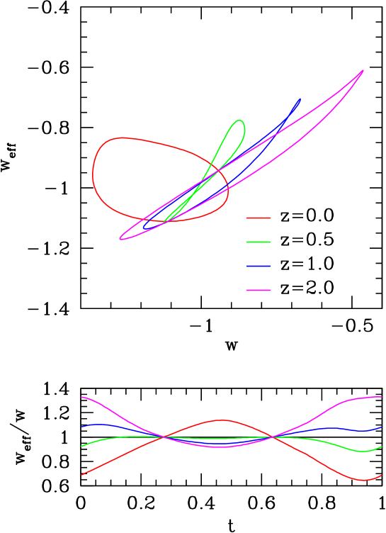
Figure 6: Bias in observational $w$ values (named here $w_{eff}$), in respect to the physical value of the state parameter, at each redshift. The points in the curves of the upper frame refer to different models at 1–$\sigma$ from the top–likelihood cosmology, discriminated by different $t$ values. In the lower frame the ratio $w_{eff}/w$ is explicitly shown as a function of $t$ .

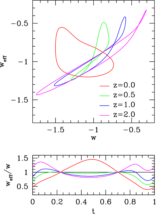
Figure 7: As Figure 6 for models at 2–$\sigma$ from the top–likelihood cosmology.

We wish to outline here a major danger that data analysis could meet in this welcome case. As a matter of fact, one could be tempted to conclude that the $w(z)$ dependence found is the physical scale dependence of the DE state parameter. Unfortunately, this could be badly untrue.

In fact, cosmic shear spectra can be easily translated into fluctuation spectra, so that observational values of $w(z)$ would correspond to $w_{eff}(z)$, not to the physical $w(z).$

How different the two behaviors can be is already represented by Figures 2–5 in this paper. But Figures 6 and 7 further illustrate this point. They show what is $w_{eff}$ when $w$ has a given value, for models laying on the 1–$\sigma$ or 2–$\sigma$ curves. Different colors in each plot correspond to different $z$’s. In the lower frame, the $w_{eff}/w$ ratio is also shown, as a function of $t$. Even in the most furtunate cases, provided that the true cosmology is not a constant–$w$ one, discrepancies are hardly below 10$\,\%$ and are greatest at $z$ approaching zero.

Another point concerning model fitting is that a systematic mapping of (reasonable) dDE cosmologies, in order to fit future data, is apparently unnecessary. At each $z$, in fact, there will be a constant–$w$ model able to fit any dDE cosmology. dDE will then be revealed by the $w$ dependence on $z$, as above outlined. At present, well approximated analytical expressions of $P(k)$, at different $z$, are provided by the so–called Halofit formulae, holding for $\Lambda$CDM cosmologies [12]. Some attempt to generalize Halofit to constant $w\neq-1$ were also performed [13], but they do not cover the desired parameter ranges. Our conclusion is that it will be important to extend Halofit to constant–$w$ cosmologies, for the whole range of (reasonable) cosmological parameters; this will enable us to fit future cosmic shear data without any substantial restriction on the $w(a)$ behavior.

5 Acknowledgments

Thanks are due to Silvio Bonometto for a number of discussions, for providing some numerical tools and discussing the final text of this article.

References

References

- Astier et al. [2006] Astier P et al. , 2006 Astronom. Astrophys. 447 31
- Riess et al. [2007] Riess A G et al. , 2007 Astrophys. J. 659 98
- Komatsu et al. [2008] Komatsu E et al. , 2008 Preprint 0803.0547v1.
- Colombo & Gervasi [2006] L. Colombo L & M. Gervasi, 2006 J. Cosmol. Astropart. Phys. 10 001
- La Vacca & Kristiansen [2009] G. La Vacca & J. R. Kristiansen, 2009 J. Cosmol. Astropart. Phys. 0907, 036
- Refregier et al. [2008] A. Refregier et al. , 2008 Preprint 0802.2522
- Huterer & Tanaka [2005] Huterer D and Tanaka M, 2005 Astrophys. J. 23 369
- [8] White S, 2004 KITP Conf.: Galaxy-Intergalactic Medium Interactions Kavli Institute for Theoretical Physics
- Linder & White [2005] E. Linder and M. White, 2005 Phys. Rev. D 72, 061394
- Francis et al. [2007] M.J. Francis, G.F. Lewis & E.V. Linder, 2007 Mon. Not. R. Astron. Soc. 380 1079
- Casarini et al. [2009] L. Casarini, A. V. Macciò & S. A. Bonometto, 2009 J. Cosmol. Astropart. Phys. 3 14.
- Smith et al. [2003] Smith R E, Peacock J A, Jenkins A, White S D M, Frenk C S, Pearce F R, Thomas P A, Efstathiou G and Couchman H M P, 2003 Mon. Not. R. Astron. Soc. 341 1311
- McDonald et al. [2006] McDonald P, Trac H and Contaldi C, 2006 Mon. Not. R. Astron. Soc. 366 547