Are the spin axes of stars randomly aligned within a cluster?

Abstract

We investigate to what extent the spin axes of stars in young open clusters are aligned. Assuming that the spin vectors lie uniformly within a conical section, with an opening half-angle between $\lambda=0^{\circ}$ (perfectly aligned) and $\lambda=90^{\circ}$ (completely random), we describe a Monte-Carlo modelling technique that returns a probability density for this opening angle given a set of measured $\sin i$ values, where $i$ is the unknown inclination angle between a stellar spin vector and the line of sight. Using simulations we demonstrate that although azimuthal information is lost, it is easily possible to discriminate between strongly aligned spin axes and a random distribution, providing that the mean spin-axis inclination lies outside the range $45^{\circ}$–$75^{\circ}$. We apply the technique to G- and K-type stars in the young Pleiades and Alpha Per clusters. The $\sin i$ values are derived using rotation periods and projected equatorial velocities, combined with radii estimated from the cluster distances and a surface brightness/colour relationship. For both clusters we find no evidence for spin-axis alignment: $\lambda=90^{\circ}$ is the most probable model and $\lambda>40^{\circ}$ with 90 per cent confidence. Assuming a random spin-axis alignment, we re-determine the distances to both clusters, obtaining $133\pm 7$ pc for the Pleiades and $182\pm 11$ pc for Alpha Per. If the assumption of random spin-axis alignment is discarded however, whilst the distance estimate remains unchanged, it has an additional ${}^{+18}_{-32}$ percent uncertainty.

1 Introduction

Most authors considering the statistics of orbital or rotational stellar motion assume, where relevant, that angular momentum vectors are randomly orientated. It is possible however that the physical processes of star formation lead to a preferred axis of rotation over the scale of an individual star forming region (SFR). This might arise if the direction of average angular momentum of the molecular cloud giving rise to the SFR has a significant influence on the resulting angular momentum of individual stars – for instance, if gas were constrained to collapse along strong, large-scale magnetic fields threading the cloud.

Historically, little has been discussed either theoretically or observationally about the possibility of spin-axis alignment during star formation. This would require a relatively undisturbed collapse along magnetic field lines with little disruption from turbulence or dynamical interactions (e.g. Shu, Adams & Lizano 1987). Using circumstellar disc orientation as a proxy, some studies have suggested preferential spin alignment with the ambient magnetic field in SFRs (e.g. Tamura & Sato 1989; Vink et al. 2005), but others have found no evidence for disc axis alignment (Ménard & Duchêne 2004).

A second important reason for assessing the degree of spin-axis alignment is that measurements of projected equatorial rotation velocities ($v\sin i$, where $i$ is the unknown inclination of the spin-axis to the line of sight) and rotation periods can be combined to provide a powerful method to determine the distances (Hendry, O’Dell and Collier-Cameron 1993; Jeffries 2007a; Baxter et al. 2009), radii (Jackson, Jeffries & Maxted 2009) or star formation histories (Jeffries 2007b) of young clusters. Such statistical analyses must assume that the orientation of spin axes are random. If the spin axes in an individual cluster were in fact partially aligned, this would change the intrinsic $\sin i$ distribution for the cluster, producing biased estimates of distances, radii and age spreads.

In this paper we use published rotation data for the young Pleiades and Alpha Per open clusters to investigate to what extent spin axes may be aligned once the star formation process has finished. In Section 2 we discuss how well spin-axis orientation can be determined using measured rotation periods and projected equatorial velocities. In Section 3 we present a parameterised model for the observed $\sin i$ distribution resulting from a group of stars with partially aligned spin axes and show how well such a model can be used to determine the degree of alignment from simulated datasets. In Section 4 we compare the models with measured $\sin i$ distributions for G- and K-type stars in the Pleiades and Alpha Per clusters. Section 5 presents and discusses the results of our analyses, including new, independent estimates of the distances to these clusters under the assumption that the spin axes are randomly aligned, and in Section 6 we give our conclusions.

2 Observation of spin axes

Using current measurement techniques it is not possible to observe stellar spin-axis orientation directly. For young, magnetically active, spotted late-type stars it is possible to measure their period of rotation, $P$, from rotational modulation of their light curves and their projected equatorial velocity, $v\sin i$, from spectral line broadening. These can be used together with photometric data and an independent measure of distance to determine $\sin i$, the sine of the angle between the observer and the spin axis

$$\sin i=\frac{P}{2\pi R}\,(v\sin i)\,,$$ (1)

where the stellar radius $R$ can be estimated from the surface brightness and distance. Such observations give no information on the azimuthal direction of the spin axis, only an estimate of the inclination, $i$, which is also degenerate between $i$ and $\pi-i$.

The effect of restricting observations to measurements of $\sin i$ is illustrated in Fig. 1. The left-hand panels indicate the intrinsic distribution of spin-axis vectors. The central panels show what would be observed given the lack of azimuthal information and the degeneracy in $i$ discussed above. The right hand panels show the cumulative $\sin i$ distributions that would be observed (see section 3.1).

In the first case, where there is no preferred orientation, the uniform distribution of spin axes would be observed as a uniform inclination distribution over a hemisphere from 0 to $\pi/2$. The next case is more complicated. Here, the spin axes of a group of stars are distributed uniformly over a conical region about a central cone axis with defined inclination and azimuthal direction. This would be observed as a larger circular region on the surface of the hemisphere that is symmetric about the line of sight; the azimuthal information being lost.

The third and fourth cases show how conical regions representing the same degree of alignment would be observed at increasing average inclinations. The lack of azimuthal information causes spin axes represented by a relatively small cone area to sweep out a large area of the measured hemisphere. This concept of swept areas is approximate. A detailed treatment is given below, where the variation in number density over the swept area is modelled to calculate the cumulative probability density as a function of the opening angle of the cone, $\lambda$, and its mean inclination, $\alpha$. The point here is to emphasise that azimuthal and inclination angle degeneracies conspire, especially when convolved with measurement errors (see next section), to hamper the recovery of the underlying $\sin i$ distribution.

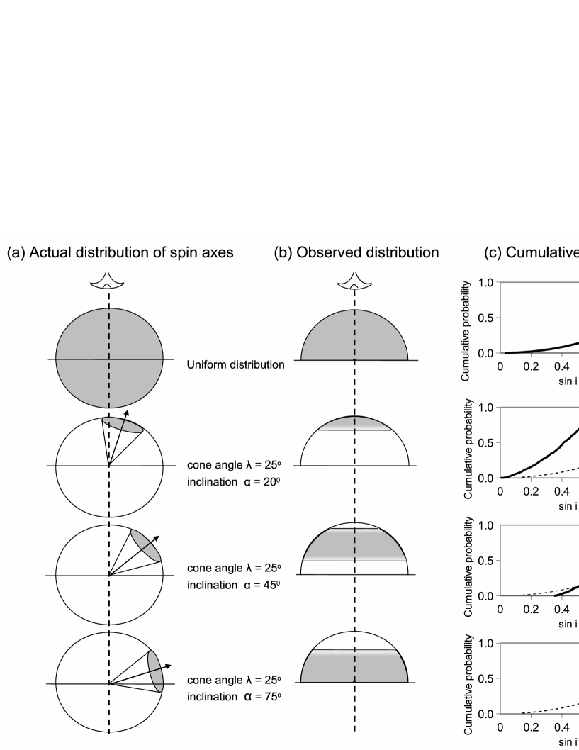
Figure 1: A schematic diagram showing (a) the distribution of spin vector orientations, (b) the corresponding distribution that would be deduced from $\sin i$ measurements and (c) the resultant cumulative probability distribution of measured $\sin i$ (solid line) compared to that found for a uniform distribution of spin axes (dashed line).

3 Modelling the ${{\large\mathbf{\sin}i}}$ distribution

We will use the term “$\sin i$ distribution” for a group of stars to express the set of numbers specifying the angle between the rotation axis and the observer’s line of sight. Two such distributions can be considered:

1. a true $\sin i$ distribution which depends only on the distribution of the spin axes of a set of stars,

2. a measured $\sin i$ distribution which depends both on the true distribution and the uncertainties and limits that apply to measurements of the base parameters used to determine $\sin i$.

3.1 The true $\sin i$ distribution

The true $\sin i$ distribution depends on the distribution of the stellar spin axes over the celestial sphere. The simplest case is a uniform (random) distribution in which case the cumulative probability distribution depends on the area of the celestial sphere between an angle 0 and $i$

$$P^{o}_{\rm true}=1-\cos i\;\;\;{\rm for}\;i=0\;{\rm to}\;\pi/2\,,$$ (2)

where the superscript $o$ denotes the case of a uniform distribution.

A simple way to represent an aligned distribution is to assume that spin vectors are uniformly distributed over a conical solid angle and zero elsewhere (see Fig. 1). The cone angle, $\lambda$, which corresponds to half the opening angle, determines the degree of alignment. A small cone angle means stars have nearly parallel spin. A large cone angle ($\lambda\approx\pi/2$) corresponds to a uniform distribution. The mean inclination of the stars within the cone is represented by $\alpha$.

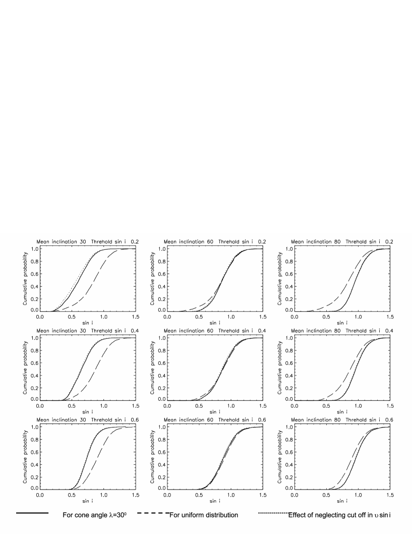
Figure 2: Simulations of the cumulative probability distributions of observed $\sin i$ assuming normalised uncertainties $\delta_{PV}=\delta_{AD}=0.1$ and a distribution of spin-axis orientations that is either a uniform (random) or is aligned within a cone angle $\lambda=30^{\circ}$. The rows show results for mean inclinations of $\alpha=30^{\circ}$, $60^{\circ}$ or $80^{\circ}$. The columns show the effects of altering $\sin i_{\rm min}$. The dotted line shows the effect of setting $(v\sin i)_{\rm min}=0$. Note the value of $\sin i$ can exceed unity due to uncertainties in the measured parameters used to determine $\sin i$.

The equivalent $\sin i$ distribution can then be calculated using a Monte Carlo method as follows. A set of spin axes are specified at angles $\theta_{n}$ and $\phi_{n}$, relative to the cone axis. The cumulative probability distribution depends on the angle between the cone axis and spin axis, $\theta_{n}$, as

$$P(\theta)=(1-\cos\theta)/(1-\cos\lambda)\;\;\;{\rm for}\,\theta=0\;{\rm to}\;\lambda$$ (3)

and random values of $\theta_{n}$ are generated as

$$\theta_{n}=\cos^{-1}(1-R_{n}(1-\cos\lambda))$$ (4)

where $R_{n}$ is a random number between 0 and 1. The probability distribution of the angle $\phi$ around the cone axis is uniform, allowing random values of $\phi$ to be generated as $\phi_{n}=2{\pi}R^{\prime}_{n}$ (where $R_{n}$ and $R^{\prime}_{n}$ are different random numbers). The inclination relative to the line of sight is calculated by considering the triangle formed by unit vectors along the spin axis and the line of sight with respect to the cone axis. As the line of sight is at an angle $\alpha$ with respect to the cone axis, then

$$\cos i_{n}=\sin\alpha\sin\theta_{n}\cos\phi_{n}+\cos\alpha\cos\theta_{n}\,.$$ (5)

Since measurements of inclination derived from projected rotational velocities cannot distinguish between $i$ and $\pi-i$, the effective value of $\sin i$ is given by

$$\sin i_{n}=\sin(\cos^{-1}(|\sin\alpha\sin\theta_{n}\cos\phi_{n}+\cos\alpha\cos\theta_{n}|))\,.$$ (6)

A Monte Carlo method is used to determine the expected distribution of $\sin i$, for a given $\lambda$ and $\alpha$. A set of $\sin i$ values is evaluated for random values of $\theta$ and $\phi$. The results are then ordered to define the cumulative distribution function of $\sin i$. This cumulative distribution can then be used to determine a representative set of $\sin i$ values by generating random numbers between 0 and 1.

The right hand panels in Fig. 1 show the cumulative $\sin i$ probability distributions calculated for a uniform distribution and for well aligned distributions with $\lambda=25^{\circ}$ and various values of $\alpha$. For $\lambda=25^{\circ}$ the true $\sin i$ distribution is significantly different from that of a uniform distribution. Thus with sufficient $\sin i$ measurements it should be possible to differentiate between well-aligned and uniform distributions, irrespective of the inclination $\alpha$.

Things become less clear when $\lambda$ is increased to, say, $60^{\circ}$. In this case the results at low $(\alpha\simeq 20^{\circ})$ and high $(\alpha\simeq 75^{\circ})$ inclinations could still be differentiated from a uniform distribution. However, at intermediate inclinations the $\sin i$ distribution becomes quite similar to that for a uniform distribution. Thus a weakly aligned spin-axis distribution with large $\lambda$ might only be discernible if its mean inclination is either low or high.

Of course, these simple considerations have so far ignored the alterations to the observed $\sin i$ distribution that are imposed by selection effects in the data and by measurement uncertainties, which are discussed in the next section.

3.2 Measured ${\bf\sin i}$ distribution

An expression for the observed value of $\sin i$ is obtained from equation 1 and by assuming that the stellar radius is proportional to the product of its angular diameter and distance.

$$\sin i_{\rm obs}=k\,P_{\rm obs}(v\sin i)_{\rm obs}/(A_{\rm obs}D_{\rm est})\,,$$ (7)

where $k$ is a constant (appropriate to the units used) of

$$k=A_{\rm true}D_{\rm true}/(P_{\rm true}v_{\rm true})\,,$$ (8)

$P_{\rm obs}$ is the observed period of a star, $(v\sin i)_{\rm obs}$ is its measured projected equatorial velocity, $A_{\rm obs}$ its angular diameter (derived from a magnitude and colour via a Barnes-Evans relation – see section 4.2) and $D_{\rm est}$ is the distance to the star estimated by some independent method.

Uncertainties in the observed $v\sin i$, period, angular diameter and distance estimate can be represented as Gaussian distributions with normalised standard deviations of $\delta_{p}$, $\delta_{v}$, $\delta_{A}$ and $\delta_{D}$, such that $P_{\rm obs}=P_{\rm true}(1+\delta_{P}U)$ etc. where $U$ is a random numbers drawn from a Gaussian distribution with mean of zero and unit standard deviation. Hence we can write

$$\sin i_{obs}=\sin i_{true}\left(\frac{1+\delta_{PV}U_{1}}{1+\delta_{AD}U_{2}}\right)$$ (9)

where $\delta_{PV}=\sqrt{\delta_{P}^{2}+\delta_{V}^{2}}$,  $\delta_{AD}=\sqrt{\delta_{A}^{2}+\delta_{D}^{2}}$

and $U_{1}$ and $U_{2}$ are different random numbers with a mean of zero and a standard deviation of 1. For the moment $\delta_{PV}$ and $\delta_{AD}$ can be considered as empirically derived constants. Their values are discussed in section 4.6.

In addition to measurement uncertainties there are thresholds below which either period or $v\sin i$ cannot be measured. These thresholds are equivalent to a lower limit to $\sin i$ below which rotational modulation and periodicity would not be detected, and a resolution limit defining a threshold for $v\sin i$ detection. The latter is reasonably well defined from the observational data, but there are significant astrophysical uncertainties in the former – e.g. the latitude distribution of spots on a young, active star (see Jeffries 2007a for a discussion). We chose to represent this observational bias as a simple cut-off value $\sin i_{\rm min}$, below which a period could not be obtained for a star. In Figure 2 we show that the value of $\sin i_{\rm min}$ has a non-negligible effect on the observed $\sin i$ distribution, so it is treated as a free parameter in the following analysis and allowed to vary between zero and 0.71. That is to say we do not specify a lower limit of $\sin i$, and at worst we expect to be able to measure the period and $v\sin i$ of stars with inclinations 45^∘ and above. In section 5.1 it is shown that this is justified by the available observations.

To model the effects of the resolution limit for projected radial velocity measurement, $(v\sin i)_{\rm min}$, we require an estimate of the distribution of $v_{\rm true}$. The approach used here follows Jeffries (2007a) whereby the intrinsic $v_{\rm true}$ distribution is represented as a combination of a uniform distribution and an exponential decay. For the Monte Carlo analysis a fraction $\gamma$ of velocities are drawn from a uniform distribution between zero and $v_{\rm max}$ and the remainder from a cumulative exponential distribution of the form $P(v)=\exp(-v/\beta)$. In practice the $\sin i$ distribution is not sensitive to the exact form of the $v_{\rm true}$ distribution so parameters defining the velocity distribution ($\gamma,\beta,v_{max}$ and $v\sin i_{min}$) can be estimated by matching the distribution of $(v\sin i)_{\rm obs}$.

To take into account the threshold values of $v\sin i$ and $\sin i$ in our simulations, any realisation with $\sin i_{true}<\sin i_{\rm min}$ or $(v\sin i)_{obs}<(v\sin i)_{\rm min}$ is excluded from the $\sin i$ distribution, since these would not be present in an observed data set.

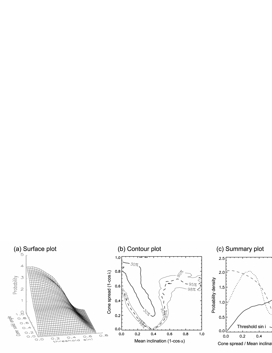
Figure 3: Analysis of the $\sin i$ distribution measured on a group of 36 stars to determine the probability density of parameters describing the underlying distribution of spin axes as a function of cone spread (or solid angle) $(1-\cos(\lambda))$ , mean inclination, $(1-\cos(\alpha))$ and threshold in $\sin i$. The measured distribution was derived for stars in Pleiades (see Table 3 and section 4.4)

Figure 2 shows Monte Carlo simulations of the cumulative $\sin i$ distribution with typical levels of uncertainty: 10 per cent in combined period and projected radial velocity and 10 per cent in combined angular diameter and distance (see section 4.6). Results are shown for three values of mean inclination, $\alpha=30^{\circ}$, $60^{\circ}$ or $80^{\circ}$ and for $\sin i_{\rm min}=0.2$, 0.4 or 0.6. The solid lines show results for $\lambda=30^{\circ}$ and the dashed line shows the probability density for a uniform distribution of spin axes ($\lambda=90^{\circ}$). Introducing uncertainties reduces the difference in $\sin i$ distribution between the $\lambda=30^{\circ}$ cone and the uniform distribution (compare with Figure 1). However, the distributions are still quite different for either low or high values of $\alpha$. For intermediate values ($45^{\circ}\leq\alpha\leq 75^{\circ}$) it may still be possible to resolve the difference provided $\sin i_{\rm min}\approx 0.2$. Above this, the effect of increasing $\sin i_{\rm min}$ is to compress the distributions along the $\sin i$ axis effectively erasing the distinction between the aligned and random spin-axis distributions.

These results were calculated for a velocity distribution described by $\gamma=0.33$, $\beta=37$ km s^-1, $v_{\rm max}=140$ km s^-1 and $(v\sin i)_{\rm min}=3.6$ km s^-1 (appropriate for the Pleiades – see section 4.5). Also shown as a dotted line in Figure 2 are results calculated assuming no lower cut off in $v\sin i$. This produces only small changes in the modelled $\sin i$ distributions, justifying the use of a simple representation for the velocity distribution.

3.3 Fitting parameters to measured distributions

In our models there are three unknown parameters that define the observed $\sin i$ distribution – the opening half-angle of the cone, $\lambda$, that describes the degree of spin-axis alignment, the mean inclination $\alpha$ and $\sin i_{\min}$ which we will refer to as $\tau$. The next step in the analysis is to determine how the $\sin i$ distribution of a group of stars can be analysed to determine the underlying parameters $(\lambda,\alpha,\tau)$, of which we are most interested in determining $\lambda$.

Elements of the measured $\sin i$ distribution are ordered to produce a cumulative distribution function. This is then compared with a Monte Carlo model $\sin i$ distribution using a Kolmogorov-Smirnov (K-S) test. This gives an estimate of the probability that the measured data could be drawn from the same distribution as the model data set. The larger the estimated probability the more likely it is that the model parameters ($\lambda$, $\alpha$, $\tau$) represent the measured data.

The K-S probability is calculated for all values of $\lambda_{i},\alpha_{j},\tau_{k}$ and normalised by setting the integral over all parameter space to be unity, to give the probability matrix $\Delta^{m}(\lambda_{i},\alpha_{j},\tau_{k})$. To visualise results it is useful to sum over one or two of the independent variables to produce contour plots of probability density for two parameters of interest or line plots for one parameter of interest respectively. Figure 3 shows typical results for a set of 36 stars in the Pleiades (see section 4). Figure 3a shows a surface plot of the probability density as a function of “cone spread”, (or cone solid angle – defined as $1-\cos\lambda$), and the $\sin i$ threshold, $\tau$. These results show that there is a range of $\lambda$ and $\tau$ that give reasonable fits to the measured data. Very roughly, they indicate that the cone spread lies between $\approx$0.4 and 1 (corresponding to $55^{\circ}<\lambda\leq 90^{\circ}$) and that $\tau<0.5$. The modelling suggests then that the measured data are most likely drawn from a nearly uniform distribution, but that there is still a finite probability of a partially aligned distribution of spin axes.

To put this on a quantitative basis we can look at a a contour plot of cone spread against $1-\cos\alpha$ (Fig. 3b). The contours contain the labelled percentage of the summed, normalised K-S probability. This shows that if the cone inclination is small or close to unity ($\alpha$ close to $0^{\circ}$ or $90^{\circ}$) then the results could only be consistent with a large cone spread $1-\cos\lambda>0.6$, or $\lambda>66^{\circ}$). However, for intermediate values of inclination the measurements are consistent with almost any value of cone spread. Figure 2 shows why this is. At intermediate inclinations there is a much smaller difference between the $\sin i$ distributions for well-aligned and randomly orientated spin axes.

Figure 3c shows a summary of the results for the measured $\sin i$ distribution. The solid line shows the probability density of cone spread $(1-\cos\lambda)$. Integrating under this curve gives a $90$ per cent probability that the cone solid angle is greater than 0.21, corresponding to a cone angle $\lambda>38^{\circ}$. We can also say with 90 per cent confidence that the threshold in $\sin i$ is less than 0.5.

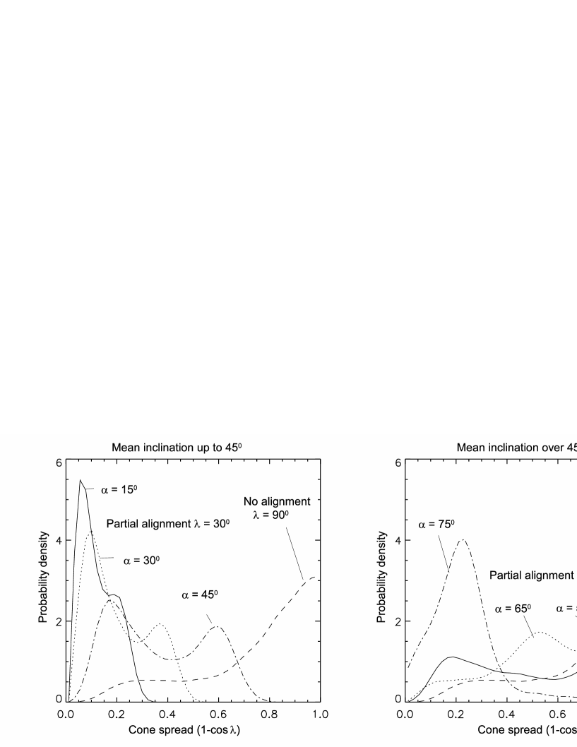
Figure 4: The probability density as a function of cone spread $(1-\cos\lambda)$ estimated from the analysis of the $\sin i$ distributions of 300 simulated stars. The curves show the results for simulated datasets with partially aligned rotation axes ($\lambda=30^{\circ}$) with different mean inclination angles, compared with a simulated dataset with random spin-axis orientation ($\lambda=90^{\circ}$, dashed line). The left hand plot show the comparison for cone inclinations, $\alpha=15^{\circ}$, $30^{\circ}$ and $45^{\circ}$. The right hand plot shows the comparison for $\alpha=55^{\circ}$, $65^{\circ}$ and $75^{\circ}$.

3.4 Conditions for discrimination of cone angle

The example in Figure 3 demonstrates how an observed $\sin i$ distribution could be analysed to investigate the underlying distribution of spin-axis orientation for a group of stars in a cluster. This section considers how useful the method might be in practice. Specifically it considers:

1. Under what conditions will this method correctly recover the underlying distribution of spin-axis orientation?

2. What effect does sample size and uncertainty in individual $\sin i$ measurements have on the accuracy of the method?

To address the first question the Monte Carlo method is used to generate $\sin i$ distributions for two scenarios. The first represents the case where there is significant alignment of spin axes of stars in the cluster corresponding to $\lambda=30^{\circ}$. The second case represents a uniform distribution with $\lambda=90^{\circ}$. The $\sin i$ values are produced for sets of 300 stars with typical levels of uncertainty in $(\sin i)_{\rm obs}$, namely $\delta_{PV}=\delta_{AD}=10$ per cent, a representative $v_{\rm true}$ distribution and $\tau=0.4$. The cumulative $\sin i$ distributions are then analysed using the method described above to determine the probability density of cone spread, which should reflect the underlying distribution of spin axes.

The results are shown in Fig.4 for increasing values of $\alpha$. For low values of $\alpha$ ($<45^{\circ}$) the distribution is peaked towards low values of $1-\cos\lambda$, roughly corresponding to the input value of $\lambda$. At high values of $\alpha$ ($\geq 75^{\circ}$) this is also the case. However at intermediate values, the probability density becomes more uniform indicating that the $\sin i$ distribution could have arisen from almost any value of $\lambda$. The reasons for this were discussed in section 3.1 and need not be repeated here.

Where the probability density falls to zero at one end or other of the distribution, we can calculate limits on $\lambda$. For example, integration under the dashed line in Fig. 4 (where the input value of $\lambda$ was $90^{\circ}$) returns a 90 per cent confidence limit that $\lambda>50^{\circ}$. This limit is the figure of merit we choose to characterise a $\sin i$ distribution, indicating whether it results from an aligned distribution or not.

Table 1: Lower limit to the cone angle, $\lambda$, found from input simulated datasets with random spin-axis orientation.

No. stars	Threshold in	90 per cent lower limit
analysed	$\sin i$, $\tau$	of cone angle, $\lambda$ (deg)
Uncertainties,	$\delta_{PV}$ & $\delta_{AD}$	0.10 & 0.10	0.15 & 0.15
10	$\sin i>0.2$	$>30\pm$6	$>29\pm$7
	$\sin i>0.4$	$>30\pm$4	$>29\pm$5
30	$\sin i>0.2$	$>39\pm$4	$>33\pm$9
	$\sin i>0.4$	$>36\pm$6	$>33\pm$5
100	$\sin i>0.2$	$>46\pm$6	$>40\pm$7
	$\sin i>0.4$	$>47\pm$2	$>48\pm$3
300	$\sin i>0.2$	$>47\pm$3	$>48\pm$5
	$\sin i>0.4$	$>49\pm$5	$>44\pm$5

To determine the effect of sample size, measurement uncertainties and the threshold $\tau$, a range of Monte Carlo simulations were performed. These were divided into runs with $\lambda=90^{\circ}$ and $\lambda=30^{\circ}$. The results of analysing the $\sin i$ distributions are listed in Tables 1 and 2.

The main conclusions from these simulations are:

1. For an input $\lambda=90^{\circ}$ (Table 1), the lower limit that can be placed on the recovered $\lambda$ value is quite insensitive to the sample size. Observing many hundreds of stars does not give much improvement over sample sizes of $\sim 30$. Neither are the results sensitive to the actual value of $\tau$ or the exact value of the measurement uncertainties.

2. For a strongly aligned distribution (input $\lambda=30^{\circ}$, Table 2) we find that upper limits to $\lambda$ are only obtained if the mean inclination $\alpha\leq 45^{\circ}$ or $\alpha\geq 75^{\circ}$. Again, the gains to be made by observing very large samples of stars are not very significant, although samples of $\sim 100$ may be required to identify a strongly aligned spin-axis distribution when $\alpha$ is large.

4 Measured $\sin i$ distributions

In this section we use the previously developed ideas to model the observed $\sin i$ distributions obtained from published measurements for stars in the young Pleiades and Alpha Per open clusters. These clusters have ages of $\simeq 120$ Myr and $\simeq 80$ Myr respectively, so many of the G- and K-stars are rotating fast enough to produce measurable rotational broadening of their spectral lines – giving $(v\sin i)_{\rm obs}$ – and produce rotational modulation caused by magnetic starspots – giving $P_{\rm obs}$. Angular diameters are determined from reported $V$ and $K$ magnitudes using a surface brightness relation calibrated by interferometry (Kervella et al. 2004).

4.1 Measured data for the Pleiades and Alpha-Per clusters

Even in the well-studied Pleiades and Alpha-Per clusters, there are surprisingly few stars where $v\sin i$ and $P$ are both known. The database for galactic open clusters (Mermilliod 1995) currently lists 296 stars in the Pleiades cluster with known $v\sin i$, and 56 with known $P$, not all of which overlap. Similarly, there are 247 stars in Alpha-Per with known $v\sin i$ and 66 with known $P$. Table 3 shows the $(v\sin i)_{\rm obs}$ and $P_{\rm obs}$ for 44 stars in the Pleiades and 38 in Alpha Per that have been identified as cluster members and for which this simultaneous information is available.

Table 3 also lists the available stellar photometry, which is subsequently used to check for unresolved binarity and estimate the angular diameters. We tabulate a mean $V$ magnitude and the (peak-to-peak) amplitude of the light curve modulation used to find the stellar rotation period. The apparent $K$ magnitudes are taken from the 2MASS catalogue (Cutri et al. 2003). A small offset is applied to convert these to the CIT photometric system used in the evaluation of angular diameter (see Section 4.2) $K_{CIT}=K_{2MASS}+0.024$, Carpenter (2001).

4.2 Estimation of angular diameter

The method used to estimate stellar angular diameter in equation 9 follows that of O’Dell, Hendry & Collier Cameron (1994). A Barnes-Evans relationship (e.g. Barnes & Evans 1976) determines the angular diameter of a star from its measured apparent magnitude and a colour index. Whilst the approach of O’Dell et al. is appropriate for the current application, the calibration data they used for the Barnes-Evans relationship has been superseded. In addition, O’Dell et al. used the $B-V$ colour index, but this is now known to be a systematically unreliable temperature indicator in magnetically active, spotted cool stars (e.g. Stauffer et al. 2003). We prefer to use $V-K$, which is potentially more precise and appears less affected by stellar activity and metallicity – the latter being a potential source of uncertainty in any calibration sample.

Table 2: Upper limit to the cone angle, $\lambda$ found from input simulated datasets with cone angle $\lambda=30^{\circ}$ and $\tau=0.4$

No. stars	Mean	90 per cent upper limit
analysed	Inclination	to cone angle, $\lambda$ (deg)
Uncertainties,	$\delta_{PV}$ & $\delta_{AD}$	0.1 & 0.1	0.15 & 0.15
10	$15^{\circ}$	$<41\pm$4	$<52\pm$8
	$30^{\circ}$	$<64\pm$12	$<65\pm$8
	$45^{\circ}$	$<74\pm$6	$<76\pm$10
	$75^{\circ}$	not resolved
30	$15^{\circ}$	$<39\pm$6	$<42\pm$4
	$30^{\circ}$	$<53\pm$6	$<54\pm$3
	$45^{\circ}$	$<72\pm$6	$<73\pm$11
	$75^{\circ}$	$<74\pm$6	$<80\pm$3
100	$15^{\circ}$	$<32\pm$1	$<34\pm$5
	$30^{\circ}$	$<51\pm$4	$<58\pm$4
	$45^{\circ}$	$<64\pm$3	$<68\pm$2
	$75^{\circ}$	$<66\pm$14	$<56\pm$16
300	$15^{\circ}$	$<30\pm$3	$<30\pm$5
	$30^{\circ}$	$<49\pm$1	$<47\pm$6
	$45^{\circ}$	$<66\pm$2	$<67\pm$3
	$75^{\circ}$	$<53\pm$17	$<53\pm$11

Table 3: Estimated values of $\sin i$ for stars in the Pleiades and Alpha Per clusters using; the Barnes-Evans relation in equation 11, a mean distance of 131.8$\pm$2.4pc and a colour excess of 0.032 for the Pleiades and a distance of 176.2$\pm$4.9pc and a colour excess of 0.10 for the Alpha Per cluster. The full table is available at Blackwell Synergy as supplementary material to the on-line version of this table.

Star	Period	$V\sin i$	Apparent	Apparent	Colour	Variation	Estimated	Estimate
Name	with ref.	with ref.	Magnitude	Magnitude	excess	magnitude	diameter	of $\sin i$
	(days)	(km/s)	$V_{mean}$	$K_{2MASS}$	$V-K_{CIT}$	${\Delta V}$	A (arcsec)
Hii 191	3.100 a	9.1 f	14.38	10.61	3.75	0.04	0.047	0.84
Hii 253	1.721 b	38.2 f	10.66	8.95	1.69	0.12	0.072	1.27
Hii 263	4.820 a	7.8 f	11.63	9.39	2.22	0.16	0.065	0.81
Hii 293	4.200 c	5.7 f	10.79	9.06	1.71	0.02	0.067	0.50
Hii 314	1.479 d	41.9 f	10.56	8.90	1.64	0.09	0.073	1.19
Hii 320	4.600 c	10.8 f	11.04	8.87	2.15	0.06	0.080	0.87
Hii 345	0.723 e	18.9 f	11.40	9.27	2.11	0.07	0.066	0.29
Hii 357	3.400 c	10.0 f	13.32	10.02	3.28	0.07	0.057	0.83
Hii 739	0.917 e	14.4 f	9.44	7.94	1.48	0.03	0.108	0.17 **
Hii 883	7.200 a	3.8 f	13.05	10.25	2.78	0.10	0.048	0.80
** Stars identified as probable binaries and excluded from the analysis of the $\sin i$ distribution
The letter following the period value denotes the reference for the period and photometric data.
The letter following the $V\sin i$ value indicates its source. The sources are as follows: a Krishnamurthi et al. (1998),
b Marilli et al. (1997), c Prosser et al. (1995), d Prosser et al. (1993), e Messina (2001), f Queloz et al. (1998),
h Stauffer & Hartmann (1987), i Soderblom et al. (1993), j Stauffer et al. (1989), k Stauffer et al. (1985)
l Prosser et al. (1993), m Prosser & Grankin (1993), n Bouvier (1996), p O’Dell et al. (1994)

Kervella et al. (2004) provide a recalibration of the Barnes-Evans relationship based on angular diameters of main sequence and sub-giant stars measured by interferometry. They give the following relationship between angular diameter, $A$, (in units of arcseconds) de-reddened magnitude, $K_{o}$ and colour $(V-K)_{o}$

$$\log(A) = (0.5170\pm 0.0017)+(0.0755\pm 0.0008)(V-K)_{o}$$ (10)

$$-0.2K_{o}\,.$$

This is valid for dwarfs of spectral type A0–M2 and has an exceptionally small intrinsic dispersion ($<1\%$), although in our case there are other sources of uncertainty in the estimated angular diameter, notably uncertainty in apparent magnitude and interstellar extinction. To allow for interstellar extinction the corrections given by Rieke and Lebofsky (1985) ($A_{V}=3.1E(B-V)$ and $E(V-K)=2.74E(B-V)$) are applied to the above expression to give

$$\log(A) = 0.5170+0.0755(V-K)-0.2K$$ (11)

$$-0.136E(B-V)\,,$$

where $V$ is the peak apparent magnitude for the variable star ($V_{mean}-\Delta V/2$) (see Table 3). The rationale here is to use the brightest value of $V$ to represent an unspotted photosphere. A mean value of colour excess, E(B-V) is used for each cluster. A value of 0.032 is taken from An, Terndrup & Pinsonneault(2007) for the Pleiades and a value of 0.10 taken from Pinsonneault et al. (1998) for Alpha Per. The expression for $\log(A)$ is quite insensitive to the magnitude of the colour excess, a very conservative uncertainty of 0.05 in $E_{B-V}$ would only change an estimated angular diameter by 1.5 per cent.

4.3 Effects of binarity

The stars in Tables 3 will inevitably include some unresolved binaries. As the effect of binarity will be to decrease the apparent magnitude (by up to 0.75 mag) and possibly redden the star with respect to the intrinsic colour and magnitude of a single star, equation 11 shows that unrecognised binarity could change the estimated angular diameter and deduced value of $\sin i$.

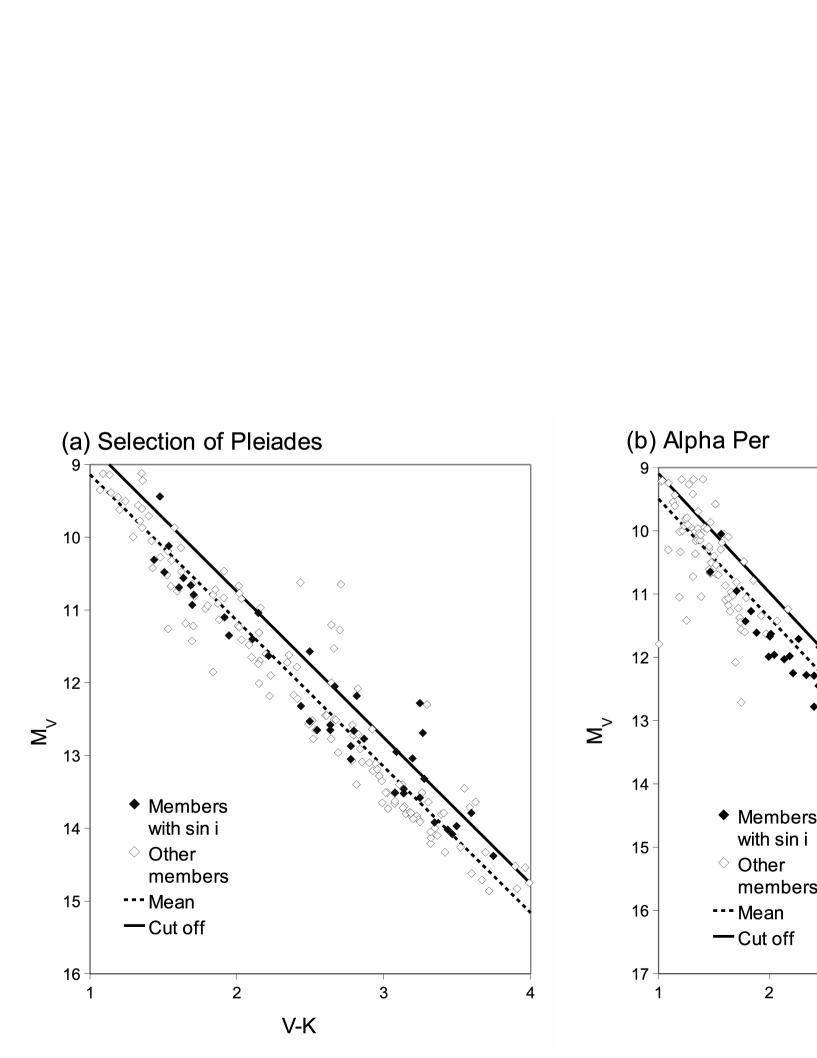
Figure 5: (a) Selection of probable binaries from stars of known period and $v\sin i$ in (a) the Pleiades and (b) Alpha Per. The solid line is located 0.4 magnitudes above the dashed regression line through all cluster members. Stars lying above the solid line are considered as probable binaries and excluded from the measured $\sin i$ distribution.

To mitigate this, probable binaries were eliminated by rejecting stars that lie significantly above the mean cluster sequence in a colour magnitude diagram. To do this in a systematic manner, reference stars identified as being cluster members in the WEBDA data base which showed 80% or greater probability of membership from proper motion measurements were plotted in a $V$ versus $V-K$ diagram (see Fig. 5). Stars lying more than 0.4 magnitudes above the linear regression line through these reference data were identified as probable binaries. When this criteria is applied to the Pleiades data in Table 3 then 8/44 of the original sample were eliminated. A similar analysis for Alpha Per eliminated 2/38 of the stars in Table 3.

4.4 Cluster distances

To calculate $\sin i$ from equation 7 we need cluster distances. We adopt $131.8\pm 2.4$ pc (distance modulus 5.60 mag) for Pleiades and $176.2\pm 4.9$ pc (distance modulus 6.23 mag) for Alpha-Per, based on multi-colour main sequence fitting (see Table 1 of Pinsonneault et al. (1998)). There has been controversy over the Pleiades distance following a much lower parallax-based measurement using the Hipparcos satellite of $120.2\pm 1.9$ pc (van Leeuwen & Hansen Ruiz, 1997; van Leeuwen, 2009). The higher distance, consistent with the results of main-sequence fitting and the distance to binary stars, has generally been been adopted in the literature. These include: a distance modulus of $5.60\pm 0.07$ mag from radial velocity and interferometric measurements of Atlas (HD 23850) (Zwahlen et al., 2004); Munari et al. (2004) used radial velocity and photometry of HD 23642 to get a distance modulus of $5.60\pm 0.03$ mag, although re-analysis of the same data by Southworth et al. (2005) gave a distance modulus of $5.72\pm 0.06$ mag; parallax measurements on three stars in Pleiades made using the fine guidance sensors on the Hubble Space Telescope (Soderblom et al., 2005) gave a distance modulus of $5.65\pm 0.02$ mag. The source of the discrepancy between the Hipparcos results and other measurement techniques remains unresolved. The distance to the Alpha-Per cluster has not been investigated to the same extent as the Pleiades. The Hipparcos distance of $172.4\pm 2.7$ pc agrees well with the main sequence fitting distance in this case.

4.5 Distributions of projected velocity

For the Monte-Carlo analysis we need an estimate of the intrinsic properties of the equatorial velocity distribution (see section 3.2). These are estimated from the observed $v\sin i$ data as follows. The maximum equatorial velocity, $v_{\rm max}$, and minimum projected velocity, $v\sin i_{\rm min}$ are taken as the maximum and minimum observed $v\sin i$ values. The true distribution of equatorial velocities is parameterised in terms of $\gamma$ and $\beta$ (see section 3.2). These coefficients are chosen to maximise the probability that a model $v\sin i$ distribution and the observed data set are drawn from a common distribution using a K-S test. Values of $\gamma=0.33$ and $\beta=37$ km s^-1 for Pleiades give a K-S probability of 0.8. Values of $\gamma=0.16$ and $\beta=54$ km s^-1 for Alpha Per give a probability of 0.7. We re-emphasise that the exact choice of these parameters has very little effect on our Monte-Carlo models of the observed $\sin i$ distribution (see section 3.2 and Fig. 2).

4.6 Measurement uncertainties

To model the measured $\sin i$ distribution we assume that statistical variations in the parameters used to derive $\sin i$ are Gaussian distributions (see equation 9) with normalised uncertainties that are derived from the measured data and published uncertainties. The source papers give uncertainties for about half the periods in Tables 3. The average of this subset of measurements gives $\delta_{P}=0.03$. The average normalised uncertainty for the velocities from Queloz el al. (2001) in Table 3 is $\delta_{V}=0.10$. Including uncertainties for data from other sources increases the average to 0.12. On the basis of these results the normalised uncertainty due to the combined effects of period and velocity, $\delta_{PV}$, is taken to be either 0.10 or 0.15.

The main source of uncertainty in estimated angular diameters is uncertainties in apparent magnitudes. Normally these should be relatively low, say $\pm 0.05$ mag for $V$ and even less for $K$. However, there is additional uncertainty for the stars used here which exhibit rotational modulation. From Tables 3 the rms magnitude variation is $\Delta V_{\rm rms}=0.09$ mag. Taking this as an upper bound for the uncertainty in both $V$ and $K$ then, from equation 16, the uncertainty in angular diameter is $\pm 5$ per cent. If we include the small intrinsic uncertainties in the Barnes-Evans relationship, $<1$ per cent (Kervella et al. 2004) and colour excess this gives a total uncertainty of about 6 per cent in the estimated radii.

The uncertainty in distance can be considered in two parts. First there is a random uncertainty due to the location of a star within the cluster. This depends on the radial depth of the cluster. We assume that the radial depth of the sample is similar to its tangential width on the sky. The Pleiades sample is located a mean distance of $0.8^{\circ}$ from the cluster centre, corresponding to a normalised distance uncertainty of 0.014. For Alpha Per the sample is scatter over a larger area, corresponding to a normalised distance uncertainty of 0.031 On this basis a value of $\delta_{AD}=0.10$ gives a conservative estimate of the combined effects of uncertainty in angular diameter and distance.

In addition to the uncertainties applied to individual stars, there is an uncertainty, $\delta_{D{\rm est}}$, in the estimate of average distance to the cluster. This produces a systematic error in the analysis, which becomes significant if the normalised uncertainty in the distance, $D_{\rm est}$ is comparable with the uncertainty in the mean value of $\sin i$ due to the combined effects of the other sources of error measured in $N$ stars.

$$\delta_{D{\rm est}}\sim\sqrt{(\delta^{2}_{PV}+\delta^{2}_{AD})/N}$$ (12)

Thus for $N=36$ stars, with $\delta_{PV}$and $\delta_{AD}$ of 10 per cent, the uncertainty in estimated distance becomes significant at a level of 2.4 per cent. As the assumed distance uncertainties to the Pleiades and Alpha Per are 1.8 and 2.8 per cent respectively, then the sensitivity of our results to variations in this value must also be considered.

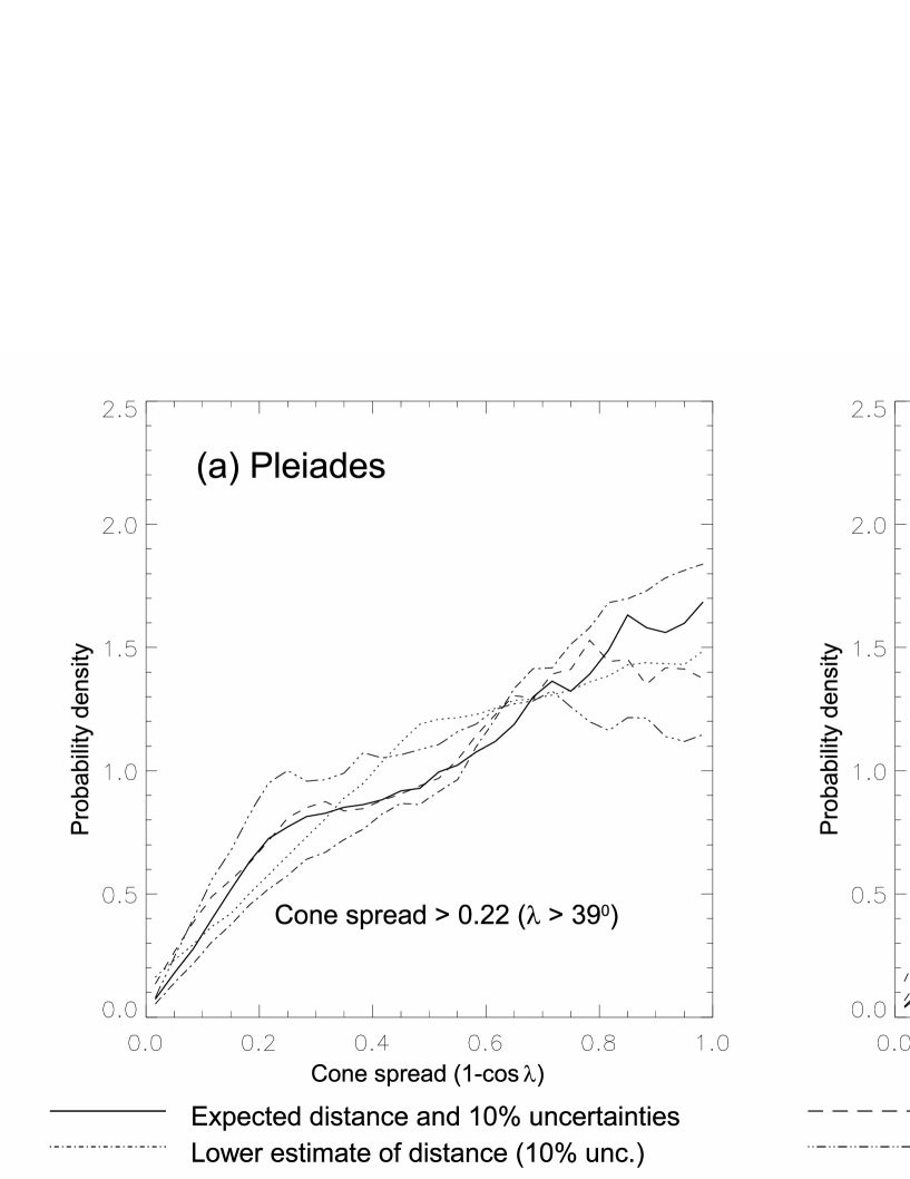
Figure 6: Analysis of measured $\sin i$ distributions for the Pleiades and Alpha Per. The solid line shows the probability density of cone spread $(1-\cos\lambda)$ that describes the underlying distribution of spin axes for normalised uncertainties of $\delta_{PV}=\delta_{AD}=0.10$. The dashed line shows the effect of increasing the normalised errors to 0.15 and 0.10. The dashed/dotted curves show the effects of varying the assumed distance to the cluster by plus or minus one standard deviation. The dotted line in the left hand plot shows the probability density of cone spread calculated assuming the a lower estimate of distance based on Hippacos data.

5 Results

5.1 Probability density of cone angle for Pleiades and Alpha Per

To investigate the degree of spin-axis alignment we look at the constraints we can place on the cone angle $\lambda$. The Pleiades stars, filtered for binaries, were modelled using the method described in section 3. Normalised uncertainties of $\delta_{PV}=\delta_{AD}=0.10$ were initially assumed. Figure 3 showed plots of the probability distributions corresponding to $\lambda$, mean inclination $\alpha$, and threshold $\sin i$ value $\tau$. Figure 6 now shows a similar plot of the probability density of cone spread ( $1-\cos\lambda$) for both Pleiades and Alpha Per, evaluated for different levels of combined uncertainty in period and $v\sin i$ and for the cluster distances fixed at the assumed value plus or minus their formal error bars.

For both clusters there is a clear increase in probability for larger values of cone spread $(1-\cos\lambda)$ and therefore of $\lambda$ itself. A qualitative comparison with the simulations shown in Fig. 4 demonstrate that this behaviour suggests a random spin-axis orientation, rather than one with a small $\lambda$. By integrating the probability distributions we can say with 90 per cent confidence that $\lambda>39^{\circ}$ for the Pleiades and $\lambda>42^{\circ}$ for Alpha Per (see Table 5). The most likely model for both clusters is one with close-to random spin-axis alignment ($\lambda\simeq 90^{\circ}$). Figure 3b shows that a lower value of $\lambda$ would have to be “disguised” in the data by an intermediate value of alignment, $\alpha$ (see the discussion in section 3.3).

Table 4: Constraints on the cone angle, $\lambda$, and on the threshold value of $\sin i$, $\tau$ for the Pleiades and Alpha Per for different assumed distances and levels of measurement uncertainty.

Distance	Uncertainty	Cone Angle $\lambda$	Threshold $\tau$
to cluster	$\delta_{PV}$ , $\delta_{AD}$	90% limit	90% limit
Pleiades
131.8 pc	0.10, 0.10	$>39^{\circ}$	$<0.48$
131.8 pc	0.15, 0.10	$>37^{\circ}$	$<0.50$
129.4pc	0.10, 0.10	$>43^{\circ}$	$<0.48$
134.2 pc	0.10, 0.10	$>36^{\circ}$	$<0.47$
Pleiades using Hipparcos distance
120.2 pc	0.10, 0.10	$>40^{\circ}$	$<0.63$
Alpha Per
176.2 pc	0.10, 0.10	$>42^{\circ}$	$<0.52$
176.2 pc	0.15, 0.10	$>37^{\circ}$	$<0.57$
171.3 pc	0.10, 0.10	$>39^{\circ}$	$<0.51$
181.1 pc	0.10, 0.10	$>44^{\circ}$	$<0.54$

For both the Pleiades and Alpha Per we also find similar 90 per cent upper limits to $\tau$ of $\simeq 0.5$, suggesting that it is not until they have inclinations below $30^{\circ}$ that stars become unlikely to exhibit significant rotational modulation in their light curves. This supports the assumption made in section 3.2 that $\tau$ will always be less than 0.71, which corresponds to $i_{min}\leq 45^{\circ}$. Figure 6 and Table 4 also illustrate how robust these results are to alterations in our assumptions about the level of measurement uncertainty. Increasing the $\delta_{PV}$ to 0.15 does not change the probability distributions in any significant way and has only a modest impact on the 90 per cent lower and upper limits to $\lambda$ and $\tau$.

Changing the assumed distance could have more influence. In Fig.6 we show curves derived for assumed distances that are equal to the main sequence fitting distances plus or minus an error bar. For the Pleiades reducing the distance would yield a larger $\lambda$ lower limit, whereas increasing the distance hints at the possibility of some alignment though still consistent with a uniform distribution. We could discard the main-sequence fitting distance entirely and instead adopt the lower Hipparcos distance. This case is also shown in Fig.6. Whilst the cone angle probability becomes a little more uniform there is still evidence of alignment. The results in Table 4 show that $\lambda$ is still greater than $40^{\circ}$. We caution the reader that this should not be taken as evidence that these methods are insensitive to the assumed distance. As discussed in section 4.6, a distance accurate to a few per cent is really require for trustworthy constraints on $\lambda$.

5.2 New distance estimates to the Pleiades and Alpha Per

If we adopt the assumption that the spin-axes really are randomly oriented then we can derive an independent distance(O’Dell et al. 1994). This provides a first check for possible alignment of spin axes since if the distance derived assuming random orientation does not agree with the established distance there is a strong indication of partial alignment which can be investigated using the method described above. Note the converse is not true since a matching distance can also be produced by a partially aligned cluster at a favorable average inclination ($45^{\circ}$ to $75^{\circ}$).

Combining the $v\sin i$ and period data in Table 3 gives an estimated distance to the Pleiades of $133\pm 7$pc. This is in good agreement with the value found from main sequence fitting of $131.8\pm 2.4$ pc adopted in the last section (Pinsonneault et al., 1998), but significantly higher than the Hipparcos value of $120.2\pm 1.9$ pc (van Leeuwen, 2009). The uncertainty in our independent distance estimate is too large to completely rule out the Hipparcos result, but clearly favors the more conventional main-sequence fitting measurement (assuming that spin axes truly have a random orientation!).

For Alpha Per the data in Table 3 gives an estimated distance of $182\pm 11$pc. This agrees well with the distance given by main sequence fitting, $176.2\pm 4.9$ pc, and within one standard deviation of the value derived from the new reduction of Hipparcos data, $172.6\pm 2.8$ pc (van Leeuwen, 2009).

It is also interesting to compare these results with those of O’Dell et al. (1994) who used a similar technique to find the distance to these clusters, but with smaller samples. They found distances of $132\pm 10$ pc and $186\pm 12$ pc for the Pleiades and Alpha Per respectively. To some extent the agreement here is fortuitous. O’Dell et al. used an older Barnes-Evans calibration based on $B-V$ data and did not exclude probable binaries. Using our data set with the surface brightness $B-V$ relations of Kervella et al. (2004) would tend to increase the estimated cluster distance, whereas our exclusion of possible binaries reduces it.

5.3 Biases in estimated cluster distances

If the distribution of spin-axis orientation were not random then there may be a systematic error in the distances estimated in the last section and it might be possible to obtain agreement with the Hipparcos distance for the Pleiades. In Fig. 7 we show the results of Monte-Carlo simulations which investigate by what factor we would overestimate the true distance for the cases of two aligned distributions with $\lambda=15^{\circ}$ and $\lambda=45^{\circ}$ respectively, if we were to analyse the $\sin i$ distributions under the assumption of random alignment. In each case we have assumed that the mean inclination $\alpha$ is randomly distributed between a maximum value of $90^{\circ}$ and a minimum value of $15^{\circ}$ which corresponds to spin-axes which almost point towards the observer. We take $15^{\circ}$ as a practical minimum value because for lower values we simply wouldn’t be able to measure any $v\sin i$ values.

The mean x-axis values for the two distributions shown in Fig.7 are both 0.99. That is, the distance we would estimate (on average) is not significantly biased by the assumption of random spin-axis alignment. However, the widths of these distributions imply a significant additional scatter. Clusters in which the spin-axes were highly aligned ($\lambda=15^{\circ}$), with a mean inclination $\alpha=15^{\circ}$ would have their distances under-estimated by a factor of two. If on the other hand the mean inclination were to take its maximum value of $\alpha=90^{\circ}$, the distance would be overestimated by a maximum factor of about 1.2.

If $\lambda$ is not $90^{\circ}$, then it seems reasonable to take a 68 per cent confidence interval about the mean of the $\lambda=15^{\circ}$ distribution in Fig. 7 as an indication of the maximum additional systematic error in the estimated distance that is introduced by assuming random spin-axis orientation. Quantitatively, this amounts to an additional uncertainty of ${}^{+18}_{-32}$ percent.

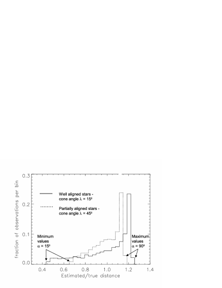
Figure 7: Possible bias in the estimated distance to a cluster for well ($\lambda=15^{\circ}$) and partially aligned ($\lambda=45^{\circ}$) stars in a cluster. The histogram shows the frequency of estimates of distance (normalized to the true distance) assuming that the mean axis of alignment of the cluster is oriented randomly in space.

6 Discussion and Summary

The results in this paper show that analysis of the measured $\sin i$ values for groups of as few as 36 stars in a cluster can be used to investigate whether their spin axes are randomly oriented or well aligned in space. The information that can be gained is incomplete because (a) information is lost in the measurement technique, principally in the azimuthal direction of the spin axes and (b) there are significant uncertainties in the measurements of parameters used to determine $\sin i$, which blur its distribution function.

The simulations in section 3.4 and Fig. 4 indicate that a cluster of stars with random spin-axis orientation can be identified from the strong increase in probability density with cone angle. In some cases it is easy to distinguish this from a well-aligned distribution of spin axes, but it depends on the average inclination, $\alpha$, of the aligned spin axes. If $\alpha\leq 45^{\circ}$ then a well aligned distribution produces a distinctive probability density that falls to zero for $\lambda<90^{\circ}$. However, if $45<\alpha<75^{\circ}$ then the probability density of $\lambda$ becomes quite flat, giving no clear indication of the underlying distribution of spin axes. The simulations presented in section 3.4 also show that there are only modest gains to be made by observing very large samples of stars The exception would be a set of stars with a well-aligned distribution with a high mean inclination ($\alpha\geq 75^{\circ}$). In this case a relatively large sample ($\approx 100$ stars) is required to clearly identify the high degree of alignment.

The first application of this technique using data for 36 stars in the Pleiades and Alpha Per is encouraging. For both clusters there is a clear increase in probability density with cone angle, entirely consistent with random spin-axis orientation. However, we cannot rule out partial alignment of the spin axes, but place 90 per cent lower limits of about $\lambda>40^{\circ}$ for both clusters. Values of $\lambda$ that are much less than $90^{\circ}$ could only be disguised in the data if the mean inclination were between $45^{\circ}$ and $75^{\circ}$ . Our results also show that the analysis method is relatively insensitive to the exact levels of measurement uncertainty and small changes in the assumed mean distance to the cluster. These results show that for the method of analysis to be effective the average distance to the cluster taken from independent measurements needs to be well defined with a normalised uncertainty of a few per cent or better.

Should it turn out to be possible to assume that spin axes are always randomly directed within a cluster, then this allows measurements of average stellar distances, radii and age spreads. In this paper we have used this technique to derive new distance estimates for the Pleiades and Alpha Per of $133\pm 7$ pc and $182\pm 11$ pc respectively. These values are in good agreement with the main sequence fitting distances to these clusters. The Pleiades result is marginally higher than the Hipparcos parallax-based distance. If larger samples of stars could be measured, then unlike the test for random spin alignment, there are significant gains (improving by a factor of approximately $\sqrt{N}$) to be made in the precision of the mean $\sin i$ value, which in turn determines the statistical precision of the distance estimate. As there are far more $v\sin i$ measurements than known periods in both the Pleiades and Alpha Per, it would be a fruitful project to search for more rotation periods in both these clusters. However, if spin-axis orientation cannot be assumed random, then although the estimated distance remains unbiased when analysed under the assumption of randomness, there are significant systematic errors of up to ${}^{+18}_{-32}$ percent, which render this technique ineffective as an independent means of estimating stellar radii or cluster distance.

Well defined distances should soon become available for many more open clusters following the launch of the GAIA satellite. In addition periods are now being measured systematically in nearby clusters (e.g. Aigrain et al. 2006). As these data become available it will be interesting to compare the distances derived from satellite based parallax measurement with those estimated from the measured period and rotational velocity. If all results agree within measurement errors then this would support the general assumption that spin-axes are randomly orientated in space over the scale length of a cluster. This is because it would become increasingly unlikely that the spins in all clusters were aligned, and had a mean inclination in the range $45^{\circ}$–$75^{\circ}$. Conversely, if the spin axes in some clusters are well aligned there would be a reasonable chance ($\simeq 55$ per cent if we can assume that the mean inclination from cluster-to-cluster is a random variable) of observing a cluster with an average inclination of $\leq 45^{\circ}$ or $\geq 75^{\circ}$ in which case significant alignment could be identified using the method described in this paper.

References

- Aigrain et al. (2007) Aigrain S., Hodgkin S., Irwin J., Hebb L., Irwin M., Favata F., Moraux E., Pont F., 2007, MNRAS, 375, 29
- An et al. (2007) An D., Terndrup D. M., Pinsonneault M. H., 2007, ApJ, 671, 1640
- Barnes & Evans (1976) Barnes T. G., Evans D. S., 1976, MNRAS, 174, 489
- Baxter et al. (2009) Baxter E. J., Covey K. R., Muench A. A., Furesz G., Rebull L., Szentgyorgyi A. H., 2009, ArXiv e-prints
- Bouvier (1996) Bouvier J., 1996, A& AS, 120, 127
- Carpenter (2001) Carpenter J. M., 2001, AJ, 121, 2851
- Cutri, R. M. et al. (2003) Cutri, R. M. et al. 2003, Technical report, Explanatory supplement to the 2MASS All Sky data release. http://www.ipac.caltech.edu/2mass/
- Hendry et al. (1993) Hendry M. A., ODell M. A., Collier-Cameron A., 1993, MNRAS, 265, 983
- Jackson et al. (2009) Jackson R. J., Jeffries R. D., Maxted P. F. L., 2009, MNRAS, 399, L89
- Jeffries (2007a) Jeffries R. D., 2007a, MNRAS, 376, 1109
- Jeffries (2007b) Jeffries R. D., 2007b, MNRAS, 381, 1169
- Kervella et al. (2004) Kervella P., Thévenin F., Di Folco E., Ségransan D., 2004, A&A, 426, 297
- Krishnamurthi et al. (1998) Krishnamurthi A., Terndrup D. M., Pinsonneault M. H., Sellgren K., Stauffer J. R., Schild R., Backman D. E., Beisser K. B., Dahari D. B., Dasgupta A., Hagelgans J. T., Seeds M. A., Anand R., Laaksonen B. D., Marschall L. A., Ramseyer T., 1998, ApJ, 493, 914
- Marilli et al. (1997) Marilli E., Catalano S., Frasca A., 1997, Memorie della Societa Astronomica Italiana, 68, 895
- Ménard & Duchêne (2004) Ménard F., Duchêne G., 2004, A&A, 425, 973
- Mermilliod (1995) Mermilliod J.-C., 1995, in Egret D., Albrecht M. A., eds, Information and on-Line Data in Astronomy Vol. 203 of Astrophysics and Space Science Library, The database for galactic open clusters (BDA).. pp 127–138
- Messina (2001) Messina S., 2001, A& A, 371, 1024
- Munari et al. (2004) Munari U., Dallaporta S., Siviero A., Soubiran C., Fiorucci M., Girard P., 2004, A& A, 418, L31
- O’Dell et al. (1994) O’Dell M. A., Hendry M. A., Collier Cameron A., 1994, MNRAS, 268, 181
- Pinsonneault et al. (1998) Pinsonneault M. H., Stauffer J., Soderblom D. R., King J. R., Hanson R. B., 1998, ApJ, 504, 170
- Prosser & Grankin (1993) Prosser C. F., Grankin K. N., 1993, CFA Preprints Ser.4539, 376, 1109
- Prosser et al. (1993) Prosser C. F., Schild R. E., Stauffer J. R., Jones B. F., 1993, PASP, 105, 269
- Prosser et al. (1995) Prosser C. F., Shetrone M. D., Dasgupta A., Backman D. E., Laaksonen B. D., Baker S. W., Marschall L. A., Whitney B. A., Kuijken K., Stauffer J. R., 1995, PASP, 107, 211
- Queloz et al. (1998) Queloz D., Allain S., Mermilliod J.-C., Bouvier J., Mayor M., 1998, A& A, 335, 183
- Rieke & Lebofsky (1985) Rieke G. H., Lebofsky M. J., 1985, ApJ, 288, 618
- Shu et al. (1987) Shu F. H., Adams F. C., Lizano S., 1987, ARA&A, 25, 23
- Soderblom et al. (2005) Soderblom D. R., Nelan E., Benedict G. F., McArthur B., Ramirez I., Spiesman W., Jones B. F., 2005, AJ, 129, 1616
- Soderblom et al. (1993) Soderblom D. R., Stauffer J. R., Hudon J. D., Jones B. F., 1993, ApJs, 85, 315
- Southworth et al. (2005) Southworth J., Maxted P. F. L., Smalley B., 2005, A& A, 429, 645
- Stauffer & Hartmann (1987) Stauffer J. R., Hartmann L. W., 1987, ApJ, 318, 337
- Stauffer et al. (1985) Stauffer J. R., Hartmann L. W., Burnham J. N., Jones B. F., 1985, ApJ, 289, 247
- Stauffer et al. (1989) Stauffer J. R., Hartmann L. W., Jones B. F., 1989, ApJ, 346, 160
- Stauffer et al. (2003) Stauffer J. R., Jones B. F., Backman D., Hartmann L. W., Barrado y Navascués D., Pinsonneault M. H., Terndrup D. M., Muench A. A., 2003, AJ, 126, 833
- Tamura & Sato (1989) Tamura M., Sato S., 1989, AJ, 98, 1368
- van Leeuwen (2009) van Leeuwen F., 2009, A&A, 497, 209
- van Leeuwen & Hansen Ruiz (1997) van Leeuwen F., Hansen Ruiz C. S., 1997, in Hipparcos - Venice ’97 Vol. 402 of ESA Special Publication, The Parallax of the Pleiades Cluster. pp 689–692
- Vink et al. (2005) Vink J. S., Drew J. E., Harries T. J., Oudmaijer R. D., Unruh Y., 2005, MNRAS, 359, 1049
- Zwahlen et al. (2004) Zwahlen N., North P., Debernardi Y., Eyer L., Galland F., Groenewegen M. A. T., Hummel C. A., 2004, A& A, 425, L45