A Novel Generic Framework for Track Fitting in Complex Detector Systems

Abstract

This paper presents a novel framework for track fitting which is usable in a wide range of experiments, independent of the specific event topology, detector setup, or magnetic field arrangement. This goal is achieved through a completely modular design. Fitting algorithms are implemented as interchangeable modules. At present, the framework contains a validated Kalman filter. Track parameterizations and the routines required to extrapolate the track parameters and their covariance matrices through the experiment are also implemented as interchangeable modules. Different track parameterizations and extrapolation routines can be used simultaneously for fitting of the same physical track. Representations of detector hits are the third modular ingredient to the framework. The hit dimensionality and orientation of planar tracking detectors are not restricted. Tracking information from detectors which do not measure the passage of particles in a fixed physical detector plane, e.g. drift chambers or TPCs, is used without any simplifications. The concept is implemented in a light-weight C++ library called GENFIT, which is available as free software.

1 Introduction

Spectrometers in nuclear and particle physics have the purpose of identifying the 4-momenta and vertices of particles stemming from high-energy collisions and decays of particles or nuclei. In addition to calorimetric and other particle identification measurements, the 3-momenta and positions of charged particles are measured by tracking them in magnetic fields with the use of position sensitive detectors. Cluster finding procedures can be applied in some detectors to combine the responses of individual electronic channels in order to improve the accuracy of the position measurements. The position measurements will be called hits throughout this paper, regardless of whether they stem from a single detector channel or from a combination of several of them. Pattern recognition algorithms determine which hits contribute to the individual particle tracks. The hits identified at this stage to belong to one track then serve as the input for a fitting procedure, which determines the best estimates for the position and momentum of a particle at any point along its trajectory. A novel framework for this task of track fitting in complex detector systems is presented in this paper. It organizes the task of track fitting, i.e. the interplay between fitting algorithms, detector hits, and particles trajectories, with a minimal amount of interfaces. It is a toolkit which is independent of specific detector setups and magnetic field geometries and hence can be used for many particle physics experiments.

Tracking of particles is usually performed with a combination of different species of detectors. They can be categorized according to the different geometrical information they deliver:
1) detectors which measure the particle passage along one axis in a detector plane, e.g. silicon strip detectors or multiwire proportional chambers;
2) detectors which measure the two-dimensional penetration point of a particle through a plane, e.g. silicon pixel detectors;
3) detectors which measure a drift time relative to a wire position, i.e. a surface of constant drift time around the wire through which the particle passed tangentially, e.g. drift chambers or “straw tubes”;
4) detectors which measure three-dimensional space points on particle trajectories, like time projection chambers (TPC).
But also higher dimensional hits can occur:
5) detector systems which measure two-dimensional position information in combination with two-dimensional direction information, including correlations between these parameters. Examples could be stations of several planes of detectors of categories 1 and 2, or electromagnetic calorimeters.
For detectors which do not deliver tracking information in physical detector planes, e.g. those of categories 3 and 4, the track fitting software of many experiments resorts to simplifications, which may be justified for a particular application but prevent the usage of the same program for different experimental environments. Examples are the projection of TPC data onto planes defined by pad rows or the projection of the surfaces of constant drift time in drift chambers onto predefined planes, just leaving two lines with left-right ambiguities. This approach is problematic if the drift cells are not arranged in a planar configuration and if there is no preferred direction in which the detector is passed by the particles. Another common simplification is the treatment of two-dimensional hits (e.g. from silicon pixel detectors) as two independent one-dimensional measurements.
In the framework presented here these problems have been overcome to make optimal use of the information from combinations of all types of tracking detector systems. All detector hits are defined in detector planes. For hits in detectors which do not have physical detector planes, so-called virtual detector planes are calculated dynamically for every extrapolation of a track to a hit. The dimensionality of detector hits is not restricted. One-dimensional hits constrain the track only along the coordinate axis in the detector plane which they measure. Two-dimensional hits are used in one fitting step to constrain the track in two dimensions in their detector planes. For hits in non-planar detectors (categories 3 and 4), the hit information (e.g. a surface of constant drift time) is converted into a position measurement in a plane perpendicular to the track, so that a fit is able to minimize the perpendicular distances between the track and the position measurements. The information from hits with higher dimensionality, like those of category 5, is used in four-dimensional hits, which contain all correlations between the parameters.
Tracks of charged particles in magnetic fields are (usually) described by five parameters and a corresponding covariance matrix. The ability to extrapolate a track described by these parameters and their covariances, taking into account the effects of materials and magnetic fields, to different positions in the spectrometer is mandatory for track fitting. The concept presented here provides a well defined interface for the invocation of external programs or libraries to perform these track extrapolations. It thus allows the straightforward use of established track following codes with their native geometry and magnetic field interfaces, such as GEANE [1], which is nowadays distributed as part of CERN’s Virtual Monte Carlo (VMC) package [2]. This is the most significant difference to other projects (e.g. RecPack [3]), which offer more monolithic approaches to track fitting (e.g. defining their own geometry classes). The concept allows the simultaneous fitting of several representations of tracks to the same set of hits, i.e. to the same physical track. This flexibility is especially useful in the early phase of an experiment when different track parameterizations and extrapolation approaches can be compared with each other, in order to identify the ones with optimal performance. But also the flexible coverage of different phase space regions with different track models, or the fitting of different mass hypotheses with the same track model can be desirable. The implementation of the concept has been realized in a software toolkit called GENFIT. It is written in C++ and is designed in a fully object oriented way. It has been developed in the framework of the PANDA experiment [4], as part of the computing framework PANDAroot [5], but is now distributed as a stand-alone package [6].
GENFIT contains a validated Kalman Filter. This algorithm is commonly used for track fitting in particle spectrometers [7], since it performs much better than global minimization approaches in the presence of materials and inhomogeneous magnetic fields. The concept is however not limited to the use of the Kalman Filter. Other fitting algorithms, like Gaussian Sum Filters [8] or Deterministic Annealing Filters [9], can be implemented easily.

Section 2 describes the concept of this new approach to track fitting in detail. Section 3 points out the key features of the implementation of GENFIT. Some examples of concrete track representations, on the dimensionalities of reconstruction hits and track representations, and the interplay between them follow in Sec. 4. Simulation studies which validate the Kalman filter implemented in GENFIT are presented in Sec. 5.

2 Concept

The basic functionalities which are required for any procedure of track fitting are the extrapolation of tracks to the positions of the hits in the detectors, and the calculation of the distances between hits and tracks, i.e. the residuals. The concept discussed here divides the problem of track fitting into three main entities which are separated from each other as much as possible and interact through well defined interfaces: 1) track fitting algorithms, 2) track representations, and 3) reconstruction hits. Figure 1 shows this structure. The following sections explain these objects in detail.

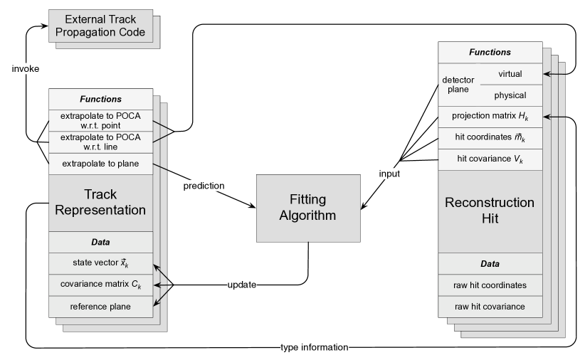
Figure 1: General structure of objects for track fitting: Fitting Algorithm, Track Representation, and Reconstruction Hit. The arrows indicate the interactions between the objects, which are described in this chapter. POCA stands for point of closest approach.

2.1 Track Fitting Algorithms

“Progressive” fitting algorithms like the extended Kalman filter [7, 10] are widely used for track fitting in high energy physics experiments. Although the track fitting concept discussed in this paper is not limited to the use of the Kalman filter, this algorithm shall serve as an example to illustrate which functionalities are generally required.
The extended Kalman filter is an efficient recursive algorithm that finds the optimum estimate $\vec{x}_{k}$ for the unknown true state vector $\hat{\vec{x}}_{k}$ of a system from a series of noisy measurements, together with the corresponding covariance matrix $C_{k}$ of $\vec{x}_{k}$. The state vector contains the track parameters and the index $k$ indicates that the state vector, and its covariance matrix are given at the detector plane of hit $k$.
Before a recursion step, the state vector $\vec{x}_{k-1}$ and covariance matrix $C_{k-1}$ contain the information of all hits up to index $k-1$. In the prediction step the state vector and covariance matrix are extrapolated to the detector plane of hit $k$ by the track following code. The predicted state vector is denoted by $\tilde{\vec{x}}_{k}$ and the predicted covariance matrix by $\tilde{C}_{k}$. This covariance matrix is the sum of the propagated track covariance matrix $C_{k-1}$ (Gaussian error propagation by transformation with the Jacobian matrix of the propagation operation $\tilde{\vec{x}}_{k}=f(\vec{x}_{k-1}))$, and a noise matrix which takes into account effects like multiple scattering and energy loss straggling. Then, the algorithm calculates the update for the state vector and the covariance matrix by taking into account the measurement $\vec{m}_{k}$:

$$\vec{x}_{k}=\tilde{\vec{x}}_{k}+K_{k}\tilde{\vec{r}}_{k}$$ (1)

$$C_{k}=(I-K_{k}H_{k})\tilde{C}_{k}$$ (2)

with the residual

$$\tilde{\vec{r}}_{k}=\vec{m}_{k}-H_{k}\tilde{\vec{x}}_{k},$$ (3)

the weight of the residual (or Kalman gain)

$$K_{k}=\tilde{C}_{k}H_{k}^{T}(H_{k}\tilde{C}_{k}H_{k}^{T}+V_{k})^{-1},$$ (4)

and the covariance matrix $V_{k}$ of the measurement $\vec{m}_{k}$. $I$ is the unit matrix of corresponding dimensionality. The projection matrix $H_{k}$ is a linear transformation from the coordinate system of the state vector $\vec{x}_{k}$, to the coordinate system of the position measurement $\vec{m}_{k}$ of hit $k$, i.e. the detector plane of the hit. A discussion about dimensions of the vectors and matrices in the above equations can be found in Sec. 4.2 together with concrete examples for the matrix $H_{k}$. The elements of the covariance matrix $C_{k}$ shrink with the inclusion of more hits, thus reducing the impact of a single hit on the value of the state vector. The $\chi^{2}$-contribution of hit $k$ is $\chi^{2}_{k}=\vec{r}_{k}^{\ T}(V_{k}-H_{k}C_{k}H_{k}^{T})^{-1}\vec{r}_{k}$ with the filtered residual $\vec{r}_{k}=\vec{m}_{k}-H_{k}\vec{x}_{k}$. It adds $\text{dim}(\vec{m}_{k})$ degrees of freedom to the total $\chi^{2}$.
After the Kalman steps have been performed on all hits of the track, the track can still be biased due to wrong starting values $\vec{x}_{0}$. This bias can be reduced by the repeated application of the procedure in the opposite order of hits, using the previous fit result as starting values for the track parameters. Before the fit is repeated, the elements of the covariance matrix have to be multiplied with a large factor ($\mathcal{O}(1000)$) in order not to include the same information in the track several times.
As can be seen in Fig. 1 the fitting algorithm operates on entities called reconstruction hits and track representations, which are detailed in the following.

2.2 Track Representations

A particle track is described by a set of track parameters and a corresponding covariance matrix, which are defined at a given position along the track. Often, the track parameters are e.g. given at a particular $z$-position. In the concept presented here, track parameters are always defined in reference planes.
In order to use a track model in a track fitter, one needs to be able to extrapolate the track parameters to different places in the spectrometer. The combination of the track parameterization and the track extrapolation functionality will be called a track representation. A track representation holds the data of the state vector $\vec{x}_{k}$, and the covariance matrix $C_{k}$ of a track, as well as the reference plane at which these are defined. Also it provides a well defined interface for the invocation of the external routines needed to extrapolate the parameters to different positions. As can be seen in Fig. 1, there are three track extrapolation functions which are needed for each track representation: Extrapolation to a plane, extrapolation to the point of closest approach (POCA) to a point, and extrapolation to the point of closest approach to a line. Fitting algorithms access the track parameters and extrapolation functions in a common way via the track representation interface without knowledge of the specific form of the track parameterization or the way the extrapolations are carried out.
Different track representations can be used in parallel. It is possible to fit the same track, i.e. the same set of hits, with different track representations simultaneously. There are several reasons why this is desirable: For low momentum particles the fitting of different mass hypotheses with the same track representation can give a clue to the particle identity via the $\chi^{2}$ of the fits, because the different energy loss for different particle masses at a given momentum leads to different extrapolations. Fitting of the same track with different parameterizations and extrapolation tools can be advantageous as well. In the early phase of an experiment one can compare different track representations to identify the ones which perform best, or there could be regions in phase space in experiments where it might not be clear beforehand which track representation will give the best results. Then one can just fit several of them simultaneously and retain the best result.

2.3 Reconstruction Hits

The object which represents a position measurement from a detector used in a track fit is called a reconstruction hit. It contains the vector of the raw measurement coordinates and its corresponding covariance matrix. As discussed in the introduction, the nature of this raw hit information can be quite diverse. It can e.g. be a direct position measurement or a drift time. As can be seen in Fig. 1, a reconstruction hit provides its detector plane, the measurement coordinates $\vec{m}_{k}$ in the detector plane coordinate system, the covariance matrix $V_{k}$ in the detector plane coordinate system, and the projection matrix $H_{k}$ to the fitting algorithm. For detectors, which measure positions in a physical detector plane (categories 1 and 2 of Sec. 1), the detector plane is identical with the physical plane.
For non-planar detectors like wire-based drift chambers or TPCs (categories 3 and 4 of Sec. 1), no such physical detector planes are defined. Instead, the concept of virtual detector planes is introduced. For space-point detectors, the track fit has to minimize the perpendicular distances of the track to the hits. Therefore, the virtual detector plane for each hit must contain the hit position and the point of closest approach of the track to the hit point. Then the residual vector which points from the hit point to the point of closest approach will be perpendicular to the track. This geometry is illustrated in Fig. 2. The orientation of the spanning vectors $\vec{u}$ and $\vec{v}$ is chosen arbitrarily in the plane. For wire-based drift detectors the virtual detector plane contains the point of closest approach of the track to the wire, and is oriented to contain the whole wire. The spanning vectors are chosen to lie perpendicular ($\vec{u}$) and along ($\vec{v}$) the wire. This geometry is shown in Fig. 3. The wire position and drift time are then measurements of $u$ (the $v$ coordinate could be measured via double-sided readout with charge sharing or time of propagation). In both cases, the orientation of the plane will directly depend on the track parameters. The consequence is that virtual detector planes have to be calculated each time a hit is to be used in a fitting step. The reconstruction hit uses the corresponding extrapolation function of the given track representation to find the point of closest approach as indicated in Fig. 1.

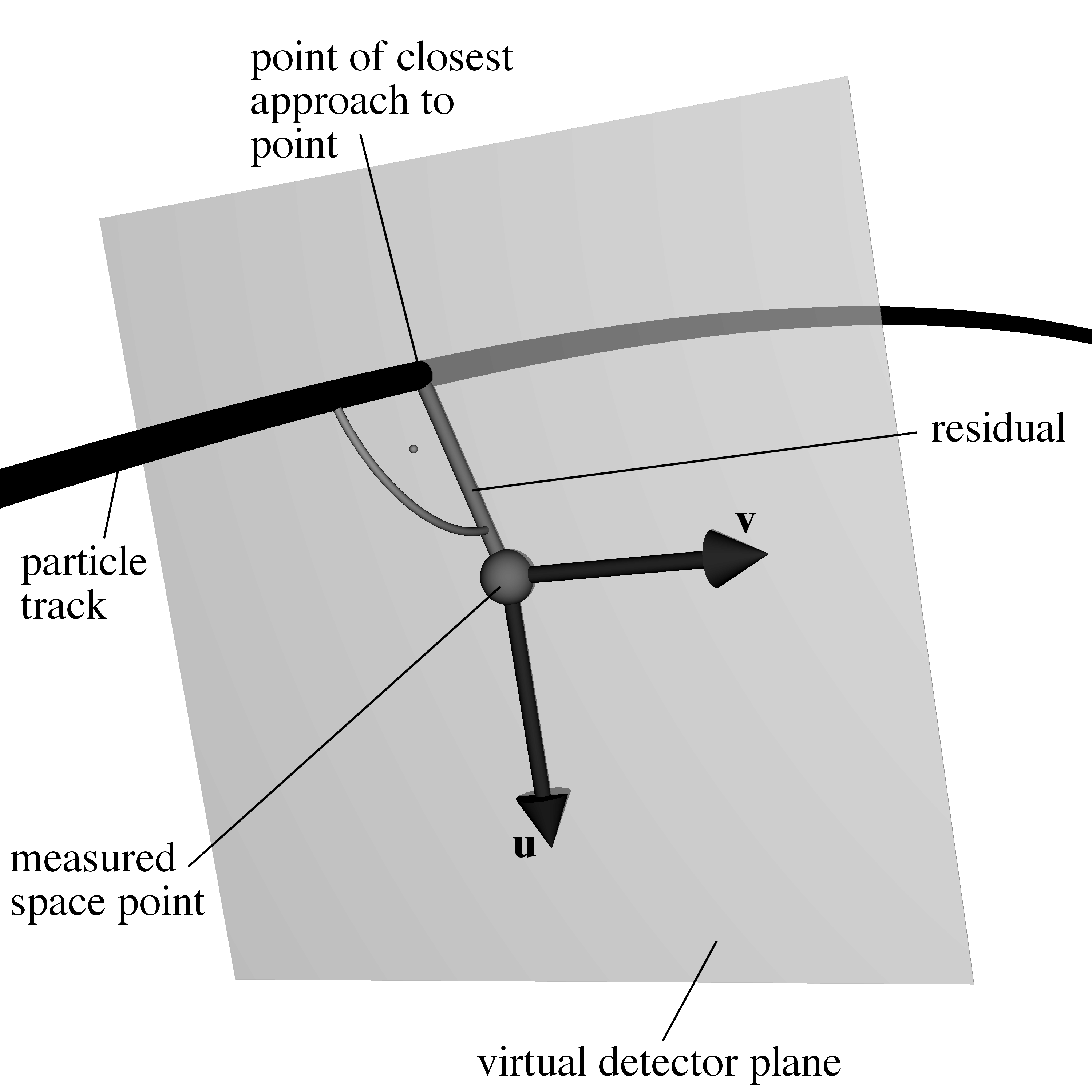
Figure 2: Virtual detector plane (spanning vectors $\vec{u}$ and $\vec{v}$) for a space-point hit.

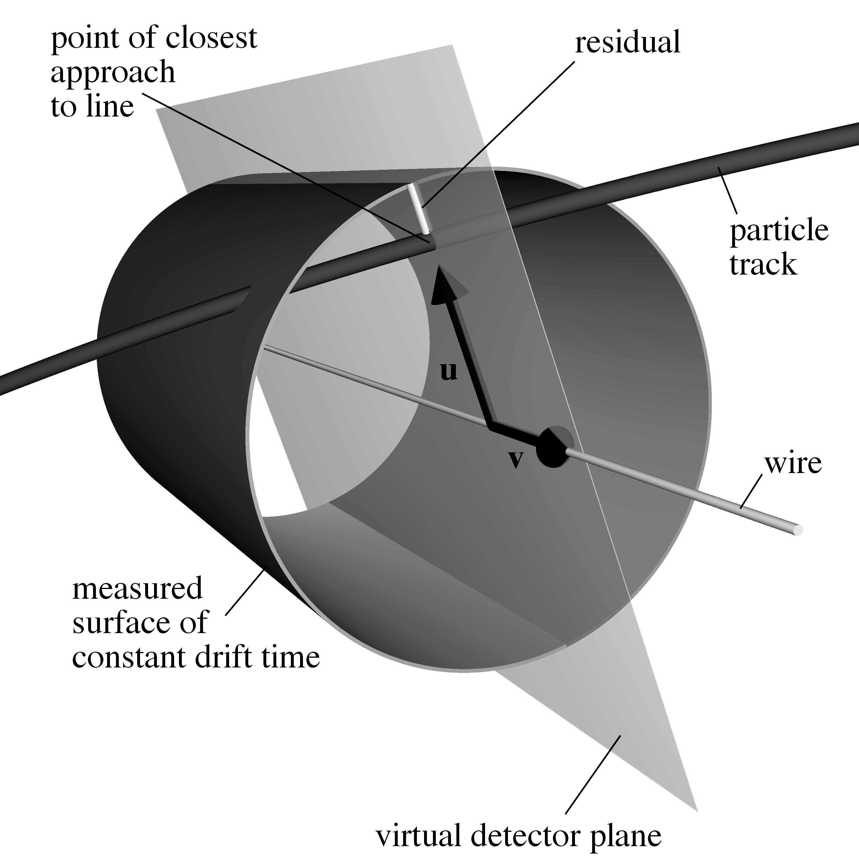
Figure 3: Virtual detector plane (spanning vectors $\vec{u}$ and $\vec{v}$) for a wire-based drift detector.

Different kinds of reconstruction hits are accessed via a common interface. When the fitting algorithm obtains the detector plane from a reconstruction hit, it does not know whether it will receive a physical or a virtual detector plane. This distinction is fully handled inside the reconstruction hit.
After the detector plane is defined, the reconstruction hit can provide the measurement coordinate vector $\vec{m}_{k}$, and the hit covariance matrix $V_{k}$. For non-planar detectors, these quantities are results of coordinate transformations into the virtual detector plane (hence the difference between the raw hit coordinates/covariance and the vector $\vec{m}_{k}$ and matrix $V_{k}$ in Fig.  1). The three-dimensional hit vector and the $3\times 3$ covariance matrix of a space-point hit are transformed into a two-dimensional vector in the detector plane and a $2\times 2$ covariance matrix. Even if the errors of the space point were uncorrelated, the matrix $V_{k}$ will in general contain a correlation, which is taken into account in the fit. For wire-based drift chambers, the drift time information is converted to a position information in the calculation of $\vec{m}_{k}$ and $V_{k}$.
The projection matrix $H_{k}$ transforms the state vector from the given track parameterization into the coordinate system of the hit. In order to determine this matrix, the concrete coordinate systems of the track representation and the reconstruction hit must be known. Since there will be typically more different types of reconstruction hits than track representations, the projection matrix is determined in the reconstruction hit object. The matrix $H_{k}$ provides the only link between a given track parameterization and the different hit coordinate systems. If a fit is performed with several track representations, the same reconstruction hit will provide a different matrix $H_{k}$ for each track representation.

3 Implementation - GENFIT

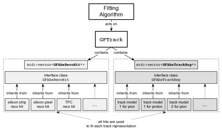
Figure 4: Class structure of GENFIT. The detailed inheritance structure of reconstruction hits is shown in Fig. 5.

The software package which implements the concept presented in this paper is called GENFIT [6]. It is completely written in C++ and makes extensive use of object oriented design. It uses the C++ standard template library [11] and the ROOT data analysis framework [12].
Figure 4 presents the general class structure of GENFIT. The classes representing the fitting algorithms operate on instances of the class GFTrack. A GFTrack object contains a std::vector<GFAbsRecoHit*> and a
std::vector<GFAbsTrackRep*>. The reconstruction hits and track representations of Secs. 2.2 and 2.3 are realized as polymorphic classes. The class GFAbsRecoHit is the interface class to the reconstruction hits, and GFAbsTrackRep is the interface class to the track representations.
The reconstruction hit objects are created from the position information acquired in the detectors. The pattern recognition algorithms, which precede the use of GENFIT, determine which of these detector hits belong to a certain track. They deliver an instance of the class GFTrackCand, which holds a list of indices which identify the hits belonging to the track. A mechanism called GFRecoHitFactory has been implemented to load the reconstruction hits into the GFTrack object.

3.1 Track Representations

In order to use a particular track parameterization for track fitting in GENFIT, one needs code which can extrapolate such track parameters, taking into account material effects on the track parameters and their covariance matrix. In order to interface the track model to GENFIT, one implements a C++ class which inherits from the abstract base class GFAbsTrackRep and provides an implementation for the virtual methods extrapolate(...), extrapolateToPoint(...), and extrapolateToLine(...). Section 4.1 presents examples of concrete track representations.

3.2 Reconstruction Hits

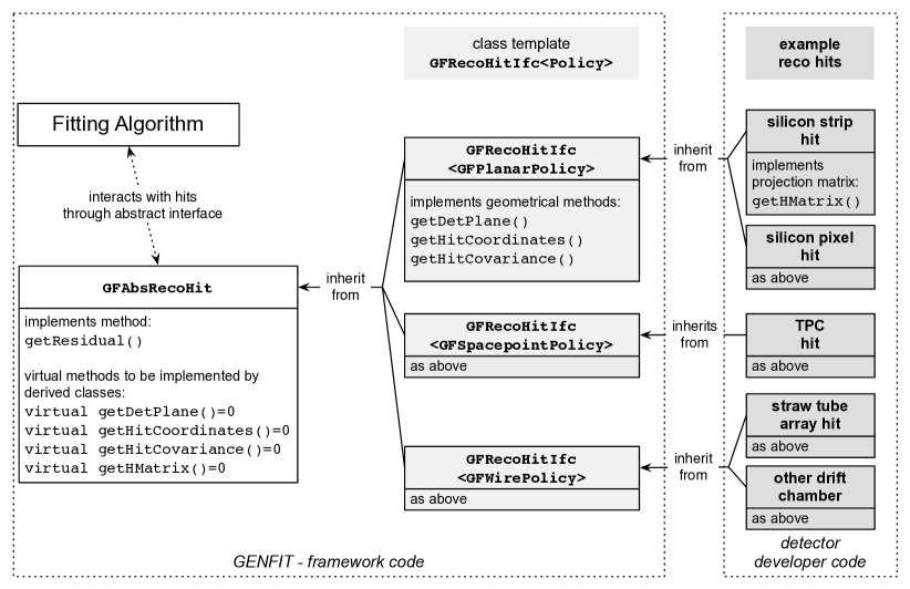
Figure 5: Inheritance structure of reconstruction hits in GENFIT.

The fitting algorithms interact with the reconstruction hits via the abstract base class GFAbsRecoHit. The reconstruction hits do, however, not inherit directly from this class, but from the intermediate interface class
GFRecoHitIfc<Policy>. This is illustrated in Fig. 5. For more information about the policy design pattern, please see [13]. There are (currently) three geometrical categories of reconstruction hits: Hits in planar detectors, space-point hits, and hits in wire-based drift chambers, which deliver their wire position and a drift time. This categorization is expressed in the code by the three different policy classes GFPlanarPolicy, GFSpacepointPolicy, and GFWirePolicy. These policy classes all implement functions for calculating or delivering the detector plane, the hit coordinates in the detector plane, and the hit covariance matrix in the detector plane. They are used to unify the geometrical properties of reconstruction hits to avoid any code duplication in the implementation of similar reconstruction hits. The latter two policies use the corresponding track representations to calculate the virtual detector planes, as detailed in Sec. 2.3.
As described in Sec. 2.1, the fitting algorithm needs a matrix $H_{k}$ which is a linear transformation from the vector space of track parameters to the coordinate system defined by the detector plane. The virtual method
GFAbsRecoHit::getHMatrix(...) is overridden in the implementations of the concrete reconstruction hits. In order to provide the correct matrix, the reconstruction hit determines the concrete type of the track representation it is asked to interact with in this particular fitting step. This type checking is represented by the lower arrow in Fig. 1. It is the only place in GENFIT where a direct type compatibility of tracks and hits is checked. A maximal modularity of the system is achieved through this mechanism. If one adds an additional track representation, it is quite obvious that one has to provide new coordinate transformations from this new parameter space into the coordinate systems in which the hits are defined.

4 Examples

4.1 Concrete Track Representations

A concrete interface to an external track propagation package which has been realized with GENFIT is the track representation called GeaneTrackRep2. It is based on the FORTRAN code GEANE. The detector geometry is included via the TGeo classes of ROOT [12] and the magnetic field maps are accessed via a simple interface class called GFAbsBField. State vectors for this track representation are defined as $\vec{x}_{k}=(q/|\vec{p}|,du/dw,dv/dw,u,v)^{T}$, where the detector plane is spanned by the vectors $\vec{u}$ and $\vec{v}$ (normal vector $\vec{w}=\vec{u}\times\vec{v}$). $q$ denotes the particle charge and $\vec{p}$ is the particle momentum. The quantitative tests of GENFIT in Sec. 5 are carried out with this track representation.
Another track representation included in the GENFIT distribution is called RKTrackRep. It was adopted from the COMPASS experiment [14] and uses a Runge-Kutta solver to follow particles through magnetic fields. It has the same state vector definition as GeaneTrackRep2. It also uses the TGeo classes for the geometry interface.

4.2 Interplay between Track Representations and Reconstruction Hits

The classes which represent the fitting algorithms just carry out their linear algebra without knowing about the dimensions of the state vectors $\vec{x}_{k}$ and the measurement vectors $\vec{m}_{k}$. The matrix $H_{k}$ is provided by the reconstruction hit class to transform state vectors and covariance matrices of a specific parameterization into the measurement vector coordinate system. This projection matrix ensures that the dimensionalities of the vectors and matrices in the fitting algorithm are compatible with each other. The following examples shall illustrate this:

1. A four-dimensional track model can be used for tracking without magnetic fields. The state vector is defined as $\vec{x}_{k}=(u,v,du/dw,dv/dw)^{T}$ for a straight line where $\vec{u}$ and $\vec{v}$ span the detector plane, and $\vec{w}=\vec{u}\times\vec{v}$ is the normal vector. A strip detector shall measure the $u$ coordinate. Then the measurement vector of equation (3), $\vec{m}_{k}$, is a scalar. The projection matrix is defined as $H_{k}=(1,0,0,0)$, so that $H_{k}\cdot\vec{x}_{k}$ is one-dimensional, just as the residual $\tilde{\vec{r}}_{k}$. The Kalman gain is a $4\times 1$ matrix, and the $\chi^{2}$-increment is correctly calculated for one degree of freedom, in the sense that $\vec{r}_{k}$ and $(V_{k}-H_{k}C_{k}H_{k}^{T})$ are scalars.

2. A pixel detector is used in combination with a five-dimensional trajectory model for charged particle tracking in magnetic fields. The detector measures the coordinates $u$ and $v$ in the detector plane, and the state vector is $\vec{x}_{k}=(q/|\vec{p}|,du/dw,dv/dw,u,v)^{T}$. The $2\times 5$ projection matrix is then:

   $$H_{k}=\left(\begin{array}[]{ccccc}0&0&0&1&0\\ 0&0&0&0&1\end{array}\right)\$$

   All matrices and vectors automatically appear with correct dimensions: $\vec{m}_{k}$ and $\tilde{\vec{r}}_{k}$ are 2-vectors, $V_{k}$ is a $2\times 2$ matrix, the Kalman gain is a $5\times 2$ matrix, and $\chi^{2}$ is a scalar which is calculated from two degrees of freedom ($\vec{r}_{k}$ is a 2-vector, and $(V_{k}-H_{k}C_{k}H_{k}^{T})$ is a $2\times 2$ matrix).
   If the next hit in the same track only measures one coordinate (e.g. $u$ in the detector plane coordinate system of the next hit) , $\vec{m}_{k}$ will be scalar, $H_{k}$ will be of dimension $1\times 5$, and there will be only one degree of freedom added to the overall $\chi^{2}$.

3. A TPC delivers space-point hits. The track model is the same as in example 2. The TPC measures three spatial coordinates but this information is transformed into a two-dimensional hit in the virtual detector plane, which is perpendicular to the track. This two-dimensional hit is treated identically to example 2. This is the desired behaviour, since measurements or errors along the flight direction do not contribute to the track fit.

5 Simulation Studies

The statistical and numerical correctness of a Kalman filter fit depends on the following items: 1) The mathematics of the Kalman filter have to be implemented correctly. 2) The projections of the covariance matrices of the hits onto the (virtual) detector planes have to be correct. 3) The propagation of the track parameters and the covariance matrix are done correctly. For the covariance matrix this means the correct estimation of the Jacobian matrices needed for the Gaussian error propagation. 4) The effects of traversed materials must be taken into account correctly: the state vector has to be modified (momentum loss) and the entries of the covariance matrix need to be increased by the addition of noise matrices (e.g. due to multiple scattering) [7]. Since the track representations are external modules, the Kalman filter and the reconstruction hit implementation in GENFIT are tested with a simplified setup, where the particles traverse a vacuum. This way, the effects number 1 to 3 are tested, while the effect number 4 is decoupled and not tested here. The setup contains a homogeneous magnetic field, since possible problems arising from field inhomogeneities would only point to problems in the external track representation module and not in the GENFIT core classes. Instead of detector responses with full digitization simulations, which result in unknown detector resolutions, known measurement errors are used.
The track representation GeaneTrackRep2 is used for these tests. The program samples 30 space points on the trajectory at distances of 1 cm, which are smeared with Gaussian distributions of known widths. Like in a TPC, the $x$- and $y$-measurements are assumed to have equal and better resolutions than the $z$-coordinate measurements ($\sigma_{x}=\sigma_{y}=1/2\cdot\sigma_{z}$). These smeared points are used in the fit as reconstruction hits based on GFSpacepointPolicy similar to TPC measurements (see Fig. 5). In front of the first hit, a reference plane is defined in which the fitted track parameters are compared to their true values to obtain residual and pull distributions. If the fit is able to correctly determine the track parameters and their errors, the pull distributions will be Gaussians of width $\sigma=1$ and of mean value $0$. Figure 6 shows the five pull distributions for the track parameters, which fulfill these criteria within the corresponding errors, proving that the non-uniform errors of the hits are taken into account correctly.
Another test is carried out with a slightly different detector geometry. Hits from 15 crossed planes of strip detectors are fitted together with 15 space-point hits. The strip hits each contribute one degree of freedom, the space-point hits each contribute two degrees of freedom (they only constrain the track in a plane perpendicular to the track), and the track parameters subtract five degrees of freedom ($15+2\cdot 15-5=40$). The $\chi^{2}$-probabilities for these fits are shown in Fig. 7. If the number of degrees of freedom is taken into account correctly, this distribution is expected to be flat. A $\chi^{2}$-test against a uniform distribution results in a $\chi^{2}/\text{n.d.f.}=87.1/99$, close to unity, as expected.
The execution time per track is 14 ms on one core of an AMD Phenom^™ II X4 940 CPU for 30 space-point hits with one forward and one backward fitting pass of all hits. Of this time, a fraction of 91% is spent in the external extrapolation routines of GeaneTrackRep2, as determined with Valgrind [15]. The GENFIT core classes have not yet been optimized for execution time, but the above result shows that optimizations would be most rewarding in the track extrapolation routines.

Figure 6: Pull distributions for the five track parameters of GeaneTrackRep2. The pull of a variable $x$ is defined as $(x_{\text{fit}}-x_{\text{true}})/\sigma_{x}$.

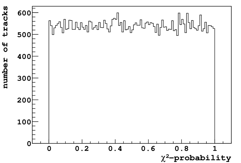
Figure 7: $\chi^{2}$-probability distribution for a series of track fits through 15 planes of strip detectors and 15 space points.

6 Conclusions and Outlook

A novel framework for track fitting in particle physics experiments has been presented in this paper. Its implementation is a C++ library called GENFIT, which is available freely. Its modular design consists of three major building blocks: Fitting algorithms, track representations, and reconstruction hits. GENFIT contains a validated Kalman filter. A standard Kalman smoother is planned to be implemented in the future, as well as other fitting algorithms. The possibility of the application of GENFIT to pattern recognition tasks seems promising and will be investigated.
The generic design of the track representation interface enables the user to use any external track following code with GENFIT. The framework allows simultaneous fits of the same particle track with different track representations. Possible applications of this feature are the fitting of different mass hypotheses with the same track model, or the test and validation of different track parameterizations and track following codes. Also the coverage of different regions of phase space with specialized track representations is an important feature in many experiments. At present, GENFIT contains two track representations which provide interfaces to the track following code GEANE and a Runge-Kutta based track extrapolation code adopted from the COMPASS experiment. New track representations which allow the use of other track following codes can be implemented in a straightforward way. The interfaces to the detector geometry and the magnetic field maps can be chosen freely and are all encapsulated in the track representation class.
The geometrical properties of reconstruction hits are not restricted in this framework. The dimensionality of hits is not fixed to particular values, and the orientation of detector planes can be chosen freely. Hits from detectors which do not measure the passage of particles in predefined planes, such as drift chambers or TPCs, are handled in the concept of virtual detector planes. This leads to a direct minimization of the perpendicular distances between the particle tracks and the position measurements from the detectors, i.e. the surfaces of constant drift time or the space points measured in a TPC.
GENFIT provides an easy-to-use toolkit for track fitting to the community of nuclear and particle physics. It is used in the PANDA computing framework. Applications in other experiments are being considered (e.g. Belle II).

References

- [1] M. Innocente, V. Mairie, E. Nagy, GEANE: Average Tracking and Error Propagation Package, CERN Program Library, W5013-E (1991).
- [2] I. Hrivnacova, D. Adamova, V. Berejnoi, R. Brun, F. Carminati, A. Fasso, E. Futo, A. Gheata, I. Gonzalez Caballero, A. Morsch, for the ALICE Collaboration, The Virtual Monte Carlo, ArXiv Computer Science e-prints, cs/0306005.
- [3] A. Cervera-Villanueva, J. J. Gomez-Cadenas, J. A. Hernando, ”RecPack” a reconstruction toolkit, Nuclear Instruments and Methods in Physics Research A 534 (2004) 180–183.
- [4] The PANDA Collaboration, Physics Performance Report for PANDA: Strong Interaction Studies with Antiprotons, ArXiv e-prints 0903.3905.
- [5] S. Spataro, Simulation and event reconstruction inside the pandaroot framework, Journal of Physics: Conference Series 119 (3) (2008) 032035 (10pp).
- [6] http://sourceforge.net/projects/genfit.
- [7] R. Frühwirth, Application of Kalman filtering to track and vertex fitting, Nuclear Instruments and Methods in Physics Research A 262 (1987) 444–450.
- [8] G. Kitagawa, The two-filter formula for smoothing and an implementation of the gaussian-sum smoother, Annals of the Institute of Statistical Mathematics 46 (4) (1994) 605–623.
- [9] R. Frühwirth, A. Strandlie, Track fitting with ambiguities and noise: a study of elastic tracking and nonlinear filters, Computer Physics Communications 120 (1999) 197–214.
- [10] R. E. Kalman, A new approach to linear filtering and prediction problems, Transactions of the ASME–Journal of Basic Engineering, Series D 82 (1960) 35–45.
- [11] B. Stroustrup, The C++ Programming Language, Special Edition, Addison-Wesley Longman, Amsterdam, 2000.
- [12] R. Brun, F. Rademakers, Root - an object oriented data analysis framework, in: AIHENP’96 Workshop, Lausane, Vol. 389, 1996, pp. 81–86.
- [13] A. Alexandrescu, Modern C++ Design: Generic Programming and Design Patterns Applied, Addison-Wesley Professional, 2001.
- [14] The COMPASS Collaboration, The COMPASS experiment at CERN, Nuclear Instruments and Methods in Physics Research A 577 (2007) 455–518.
- [15] http://valgrind.org.