Effect of random fluctuations on quantum spin-glass transitions at zero temperature

Abstract

We study the effects of random fluctuations on quantum phase transitions by the energy gap analysis. For the infinite-ranged spin-glass models with a transverse field, we find that a strong sample-to-sample fluctuation effect leads to broad distributions of the energy gap. As a result, the linear, spin-glass, and nonlinear susceptibilities behave differently from each other. The power-law tail of the distribution implies a quantum Griffiths-like effect that could be observed in various random quantum systems. We also discuss the mechanisms of the phase transition in terms of the energy gap by comparing the Sherrington-Kirkpatrick model and random energy model, which demonstrate the difference between the continuous and discontinuous phase transitions.

The quantum phase transition that could occur by changing parameters in the Hamiltonian is characterized by the closing of the energy gap between the ground and first excited states. The emergence of the gap is due to a quantum effect and we can find various new types of transitions that are absent in classical thermodynamic systems Sachdev . The situation becomes more complicated when we treat disordered systems. We need to theoretically take an average over realizations of disordered parameters. We expect that the self-averaging property holds in the thermodynamic limit and that the average model describes a real system represented by a specific realization. However, at low temperatures, the sample-to-sample fluctuations become important and lead to phenomena that can never be seen in clean systems. Actually, the gap vanishing point strongly depends on the random sample and we can hardly identify the phase transition point. In a disordered phase of the system, it is also known that physical quantities are affected by the presence of finite clusters of ordered state. This Griffiths singularity Griffiths ; McCoy is widely known in random spin systems as a general mechanism that induces random fluctuation effects. A similar effect is known in disordered electron systems as anomalously localized states in delocalized phase ALS , which shows the universality of the phenomenon for disordered systems.

The Griffiths singularity in the transverse-field Ising spin-glass model was found numerically by Rieger and Young RY , and Guo et al GBH . They found that the nonlinear susceptibility at zero temperature is divergent below a point within the quantum paramagnetic phase in two- and three-dimensional systems. It was argued that magnetically ordered clusters in a sample gives a small gap, which makes the susceptibility large. The same effect was also found by Fisher Fisher for the same model in one dimension. Although this effect was called the quantum Griffiths singularity, the formation of the ordered cluster is essentially the same as that in a classical case. It is expected to disappear at large dimensions since clusters easily form at low dimensions.

It is well known that quantum systems can be formulated using path integral formalism. Then, the quantum effect can be represented by fluctuations in an extra dimension of imaginary time and the averaging over disorder induces correlations between different times. This is a common feature that can be seen in all quantum systems with disorder. In this letter, using simple quantum spin-glass models, we consider a Griffiths-like mechanism that can persist even in infinite-ranged models without the Griffiths singularity.

We mainly discuss the Sherrington-Kirkpatrick (SK) model SK in a transverse field as one of the simplest quantum spin-glass model. The Hamiltonian is written as

$$\hat{H}=-\sum_{i<j}^{N}J_{ij}\sigma^{z}_{i}\sigma^{z}_{j}-\Gamma\sum_{i=1}^{N}\sigma^{x}_{i},$$ (1)

where $\sigma_{i}^{x,z}$ are Pauli matrices at site $i$, $J_{ij}$ are random interactions with an average $[J_{ij}]=0$ and a variance $[J_{ij}^{2}]=J^{2}/N$, $N$ is the site number, and $\Gamma$ is the transverse field. Several analyses showed that this model at zero temperature has a second-order phase transition between the spin-glass and quantum paramagnetic phases at $\Gamma/J\sim 1.4-1.5$ YI ; MH ; AR ; ADDR ; Takahashi . The SK model is the two-body interacting one, and one can generalize it into $p$-body ones. The model at $p\to\infty$ is known to be equivalent to the random energy model (REM) Derrida . Its quantum version including the transverse field can be solved exactly and shows a discontinuous transition at $\Gamma/J=\sqrt{\ln 2}\sim 0.83$ Goldschmidt . We treat both the SK model (1) and the REM since it is interesting to know the nature of the phase transition from the energy spectrum. We numerically diagonalize their Hamiltonian matrices by the Lanczos method. The number of spins, $N$, is taken up to 16. The corresponding size of the matrix is given by $2^{N}$. The ensemble average is taken over more than 20000 samples.

In Fig. 1, we show the results of the average energy gap. In the SK model, the gap vanishing point is estimated as $\Gamma/J\sim 0.6$, which is much smaller than the expected transition point. The gap vanishing point can be roughly estimated using the perturbation theory as follows. When $J=0$, energy level is exactly given by $E_{n}=-(N-2n)\Gamma$ with $n=0,1,\cdots,N$ and each level has the degeneracy $N!/(N-n)!n!$. When $J$ is included, these degeneracies are lifted to form broad distributions of energy levels. The first excited state belongs to the sector $n=1$. In this sector, the matrix element of the $N\times N$ Hamiltonian is given by $H_{ij}^{(1)}=-(N-2)\Gamma-J_{ij}$. The second term corresponds to the Hamiltonian of the Gaussian random matrix theory, and the energy levels are known to form a semicircle distribution Mehta . The width of the distribution is given by $4J$ and the first excited energy level is given by $E_{1}\sim-(N-2)\Gamma-2J$. The unperturbed ground state with the sector $n=0$ is given by $E_{0}\sim-N\Gamma$ and the energy gap is obtained as $\Delta\sim 2(\Gamma-J)$. Thus, the degenerate point is roughly estimated as $\Gamma=J$ which is modified by correlations between different sectors. Up to the second order in the perturbation theory, the degenerate point is estimated as $\Gamma/J\sim 0.85$. Since the perturbation becomes worse at small transverse fields, we cannot effectively predict the degenerate point. However, it can be definitely said that the perturbative correction decreases the value of the degenerate point and the point never approaches the phase transition point at $\Gamma>J$.

On the other hand, for the REM, we find a change in behavior around the phase transition point. The average gap becomes minimum around the point and the fluctuation also changes its behavior. This result is consistent with the analysis discussed in Ref. JKKM, , where the transition point is supposed to be equivalent to the point where the average gap becomes zero.

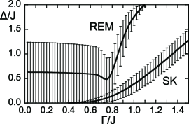
Figure 1: Average energy gap $\Delta=[E_{1}-E_{0}]$ between the ground and first excited states for the transverse SK model and REM ($N=16$). The variance of the energy gap $\pm\sqrt{[(E_{1}-E_{0})^{2}]-\Delta^{2}}$ is shown as the error bar.

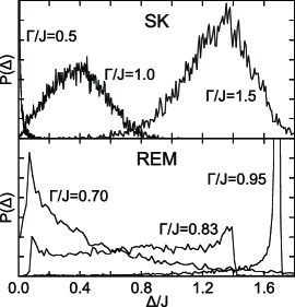
Figure 2: Gap distribution function ($N=16$).

The gap fluctuation in Fig. 1 can be clearly seen from the gap distribution function in Fig. 2. For the SK model, we find a single peak distribution with a long tail, which implies an important role of the fluctuation. In the case of the REM, we obtain more complicated distributions that are dependent on $\Gamma$. For a large $\Gamma$, we observe a single peak on the right-hand side of the distribution. When $\Gamma$ decreases, this peak decreases and another peak at the left-hand side appears. The difference between the heights of the peaks becomes smaller and changes its sign around the transition point. This behavior together with the result of the average gap implies a structural change between two different configurations at the transition point.

In the classical spin-glass theory, it is known that three types of susceptibilities, namely, linear $\chi_{\rm l}$, spin-glass $\chi_{\rm sg}$, and nonlinear $\chi_{\rm nl}$, play important roles NL ; FH . When $\Gamma=0$, the linear susceptibility is represented by the spin-glass order parameter $q=[\langle\sigma_{i}^{z}\rangle^{2}]$ as $\chi_{\rm l}=\beta(1-q)$, and the nonlinear susceptibility can be expressed by the spin-glass one as $\chi_{\rm nl}=\beta(\chi_{\rm sg}-2\beta^{2}/3)$. The phase transition characterized by the divergence of $\chi_{\rm sg}$ can be found by observing the behavior of $\chi_{\rm nl}$.

These relations are changed in quantum systems owing to the fluctuation effect. Using the spectral representation, we can write the linear susceptibility as the sum of two contributions: $\chi_{\rm l}=\chi_{\rm l}^{(\rm c)}+\chi_{\rm l}^{(\rm q)}$. The first term $\chi_{\rm l}^{(\rm c)}=\beta(\chi-q)$ corresponds to the classical part and can be treated by the static approximation BM . There is no classical counterpart for $\chi_{\rm l}^{(\rm q)}$. At zero temperature, we have

$$\chi_{\rm l}^{(\rm q)}=\frac{2}{N}\sum_{n\neq 0}\frac{\left|\langle 0|\sigma^{z}|n\rangle\right|^{2}}{E_{n}-E_{0}},$$ (2)

where $|n\rangle$ is the eigenstate with the energy $E_{n}$, $|0\rangle$ is the nondegenerate ground state, and $\sigma^{z}=\sum_{i=1}^{N}\sigma_{i}^{z}$. In the same way, the quantum parts of $\chi_{\rm sg}$ and $\chi_{\rm nl}$ are

$$\chi_{\rm sg}^{(\rm q)}=\frac{4}{N}\left(\sum_{n\neq 0}\frac{\left|\langle 0|\sigma^{z}|n\rangle\right|^{2}}{E_{n}-E_{0}}\right)^{2},$$ (3)

$$\chi_{\rm nl}^{(\rm q)}=\frac{4}{N}\sum_{n,m\neq 0}\frac{|\langle 0|\sigma^{z}|n\rangle|^{2}}{E_{n}-E_{0}}\frac{|\langle 0|\sigma^{z}|m\rangle|^{2}}{(E_{m}-E_{0})^{2}}$$

$$-\frac{4}{N}\sum_{n,n^{\prime},n^{\prime\prime}\neq 0}\frac{\langle 0|\sigma|n\rangle\langle n|\sigma|n^{\prime}\rangle\langle n^{\prime}|\sigma|n^{\prime\prime}\rangle\langle n^{\prime\prime}|\sigma|0\rangle}{(E_{n}-E_{0})(E_{n^{\prime}}-E_{0})(E_{n^{\prime\prime}}-E_{0})}.$$ (4)

The singularity of the susceptibility comes from the quantum part. It occurs when the energy gap of the first excited level $\Delta$ reaches zero. Generally speaking, $\chi_{\rm l}$, $\chi_{\rm sg}$, and $\chi_{\rm nl}$ depend on $1/\Delta^{1,2,3}$, respectively, and the energy gap distribution $P(\Delta)$ determines their critical behavior. When $\Delta$ is small, $P(\Delta)$ is assumed to have the power-law form $P(\Delta)\sim\Delta^{k}$. Then, $\chi_{\rm l}$, $\chi_{\rm sg}$, and $\chi_{\rm nl}$ diverge at $k\leq 0$, $1$, and $2$, respectively. It should be stressed here that the point where $\chi_{\rm nl}$ diverges could be different from the point where $\chi_{\rm sg}$ does.

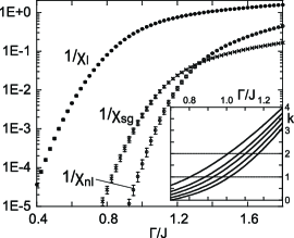
Figure 3: Inverse of the average susceptibility (quantum part) for the SK model with $N=14$. Inset: The exponent $k$ of the energy gap distribution function ($N=8$,10,12,14, and 16 from above to below). The gap exponent is fitted by $P(\Delta)\sim\Delta^{k}$ near the origin.

We plot the numerical result of the susceptibilities and the exponent $k$ in the gap distribution function for the SK model in Fig. 3. The result implies that the three susceptibilities diverge at different points, which are roughly the same as the estimates from the exponent. Although the second term in Eq. (4) is neglected in the calculation of $\chi_{\rm nl}$, we find in smaller systems that the second term does not change the divergent point. We also find $J\chi_{\rm l}\sim 2$ at a point where $\chi_{\rm sg}$ diverges, which is consistent with results of the analysis discussed in Ref. ADDR, .

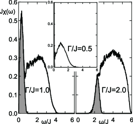
Figure 4: Local correlation function $\chi(\omega)$ for the SK model ($N=16$). The shaded areas are contributions of the first excited state.

In order to make sure that the gap between the ground and first excited states determines the divergence of the susceptibilities, we must examine the effect of higher-order excited states. For that purpose, we study the Fourier representations of a real-time correlation function including contributions from all states:

$$\chi(\omega)=\sum_{n\neq 0}\delta(\omega-E_{m}+E_{0})\left|\langle 0|\sigma_{i}^{z}|n\rangle\right|^{2}.$$ (5)

From this spectral function, we see for the SK model that the main contribution comes from $N$ levels of the sector $n=1$ if $\Gamma$ is sufficiently large. This function was analytically calculated perturbatively in ref. TT to yield a semicircle form. When $\Gamma$ decreases, a sharp peak near the origin grows and comes into contact with the vertical axis AR . As shown in Fig. 4, this peak is made from the first excited state only. We have the relation $\chi_{\rm l}^{(\rm q)}=\int d\omega\chi(\omega)/\omega$, and the behavior of $\chi(\omega)$ around the origin $\chi(\omega)\sim\omega^{k}$ determines the divergence of $\chi$. Actually, the divergence of the quantity $\int d\omega\chi(\omega)/\omega^{3}$ was used to find a phase transition ADDR . Thus, we conclude that the first excited state determines the critical behavior.

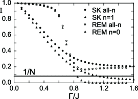
Figure 5: Inverse participation ratio (N=12). The summation over $n$ in Eq. (6) is restricted to $n=0(1)$ for a plot with the caption $n=0(1)$. The error bars are smaller than the symbols.

The above analysis cannot be applied to the REM. In this model, $\chi_{\rm l}$ and $\chi_{\rm nl}$ do not diverge. They discontinuously jump at the transition point and stay constant in the spin-glass phase. The difference can be understood from the analysis of the inverse participation ratio defined as

$$I=\sum_{n}\left|\langle n|\sigma_{i}^{z}|0\rangle\right|^{4}.$$ (6)

This quantity is estimated as the inverse of the number of excited states included in $\sigma_{i}^{z}|0\rangle$. A similar quantity was used in disordered electron systems to study the localization Wegner . As shown in Fig. 5, when $\Gamma$ is small, the difference between the SK model and the REM becomes transparent. The inverse participation ratio is close to unity in both cases and the main contribution comes from the first excited state for the SK model and from the ground state for the REM. We also see from the distribution function of $I$ that $I$ is always larger than $1/N$ which is consistent with results of the analysis of $\chi(\omega)$ for the SK model. Thus, the gap analysis above is justified for the SK model. On the other hand, the contributions of the excited states are very small and the classical analysis by static approximation is justified for the REM.

We find that the linear, spin-glass, and nonlinear susceptibilities diverge at different points, namely, $\Gamma_{\rm l}$, $\Gamma_{\rm sg}$, and $\Gamma_{\rm nl}$ respectively. $\Gamma_{\rm sg}$ corresponds to the phase transition point. Although our system size is not sufficiently large, we roughly estimate that the extrapolation to the $N\to\infty$ limit gives $\Gamma_{\rm sg}/J\sim 1.4$, which is consistent with the previous numerical results AR ; ADDR . In our numerical study, $\Gamma_{\rm nl}/J\sim 1.6$ is somewhat larger than $\Gamma_{\rm sg}$, and $\Gamma_{\rm l}/J\sim 0.9$ is close to the point where the average energy gap is zero. These behaviors can be verified by studying the distribution function of the susceptibility ${\rm P}_{\chi}(\chi)$. The power-law behavior ${\rm P}_{\chi}(\chi)\sim\chi^{-s-1}$ with $s<1$ at large $\chi$ gives the divergence of the average susceptibility. This distribution is roughly the same as the power-law distribution of the gap since $\chi_{\rm l}\sim 1/\Delta$, for example. Our detailed study will be reported elsewhere.

Although our result is very similar to that obtained in finite-dimensional systems, we cannot attribute the realization of the small gap to the presence of ordered clusters. This is because no notion of the spatial dimension exists for the present infinite-ranged model. As we mentioned earlier, the fluctuation in extra imaginary time direction can induce the quantum Griffiths-like singularity where an ordered cluster is randomly formed in its direction, which is similar to that obtained in low-dimensional classical systems. As in the finite-dimensional case Sachdev , by taking into account a rare event, we find a power-law behavior of the gap distribution function as

$${\rm P}(\Delta)\sim\int d\ e^{-c\tau}\delta\left(\Delta-\Delta_{0}e^{-\frac{c}{k+1}\tau}\right)\sim\Delta^{k},$$ (7)

where $c$, $k$, and $\Delta_{0}$ are constants and $\tau$ is the imaginary time. Instead of spatial directions in the finite-dimensional case Sachdev , a small gap is caused by a large imaginary time $\tau$ with an exponentially small probability. From the facts that the randomness is absent in the imaginary time direction and Eq. (7) is relevant only for the low-temperature limit of quantum systems, it follows that the effect should be distinguished from the Griffiths singularity. Since the present effect is present not only for the infinite-dimensional system but also for finite-dimensional ones, it is interesting to closely study how both effects are distinguished in terms of physical quantities in finite-dimensional systems.

In conclusion, we have discussed quantum spin-glass transitions in terms of the energy gap. In the SK model, our analysis implies that three susceptibilities behave differently from each other and diverge at different points, which must be confirmed by further studies. The result can be characterized by a power-law behavior of the distribution, which we attribute to the quantum Griffiths-like effect. In contrast to the classical Griffiths singularity, rare configurations of the quantum fluctuations play a significant role in the phase transition. On the other hand, the same mechanism cannot be applied to the REM. We have discussed conditions for this mechanism to be applied by studying several quantities. It is important to state the conditions in a more general way, which will be part of our future investigation.

We are grateful to K. Takeda for helpful discussions and comments. Y.M. acknowledges the support from the Japan Society for the Promotion of Science.

References

- (1) S. Sachdev, Quantum Phase Transitions (Cambridge University Press, Cambridge, 1999).
- (2) R.B. Griffiths, Phys. Rev. Lett. 23, 17 (1969).
- (3) B.M. McCoy, Phys. Rev. Lett. 23, 383 (1969).
- (4) B.L. Altshuler, V.E. Kravtsov, and I.V. Lerner, Pisma Zh. Eskp. Teor. Fiz. 45, 160 (1987) [JETP Lett. 45, 199 (1987)].
- (5) H. Rieger and A.P. Young, Phys. Rev. Lett. 72, 4141 (1994); Phys. Rev. B 54, 3328 (1996).
- (6) M. Guo, R.N. Bhatt, and D.A. Huse, Phys. Rev. Lett. 72, 4137 (1994); Phys. Rev. B 54, 3336 (1996).
- (7) D.S. Fisher, Phys. Rev. Lett. 69, 534 (1992); Phys. Rev. B 51, 6411 (1995).
- (8) D. Sherrington and S. Kirkpatrick, Phys. Rev. Lett. 35, 1792 (1975).
- (9) T. Yamamoto and H. Ishii, J. Phys. C 20, 6053 (1987).
- (10) J. Miller and D.A. Huse, Phys. Rev. Lett. 70, 3147 (1993).
- (11) L. Arrachea and M.J. Rozenberg, Phys. Rev. Lett. 86, 5172 (2001).
- (12) L. Arrachea, D. Dalidovich, V. Dobrosavljević, and M.J. Rozenberg, Phys. Rev. B 69, 064419 (2004).
- (13) K. Takahashi, Phys. Rev. B 76, 184422 (2007).
- (14) B. Derrida, Phys. Rev. Lett. 45, 79 (1980).
- (15) Y.Y. Goldschmidt, Phys. Rev. B 41, 4858 (1990).
- (16) M.L. Mehta, Random Matrices, 3rd ed. (Academic, New York, 2004).
- (17) T.J. Jörg, F. Krzakala, J. Kurchan, and A.C. Maggs, Phys. Rev. Lett. 101, 147204 (2008).
- (18) J. Chalupa, Solid State Commun. 22, 315 (1977); M. Suzuki, Prog. Theor. Phys. 58 1151 (1977).
- (19) K.H. Fischer and J.A. Hertz, Spin Glasses (Cambridge University Press, Cambridge, 1991).
- (20) A.J. Bray and M.A. Moore, J. Phys. C 13, L655 (1980).
- (21) K. Takahashi and K. Takeda, Phys. Rev. B 78, 174415 (2008).
- (22) F. Wegner, Z. Phys. B 36, 209 (1980).