FIRST Explorer – An innovative low-cost passive formation-flying system

Abstract

Formation-flying studies to date have required continuous and minute corrections of the orbital elements and attitudes of the spacecraft. This increases the complexity, and associated risk, of controlling the formation, which often makes formation-flying studies infeasible for technological and economic reasons. Passive formation-flying is a novel space-flight concept, which offers a remedy to those problems. Spacecraft in a passive formation are allowed to drift and rotate slowly, but by using advanced metrology and statistical modelling methods, their relative positions, velocities, and orientations are determined with very high accuracy. The metrology data is used directly by the payloads to compensate for spacecraft motions in software. The normally very stringent spacecraft control requirements are thereby relaxed, which significantly reduces mission complexity and cost. Space-borne low-frequency radio astronomy has been identified as a key science application for a conceptual pathfinder mission using this novel approach. The mission, called FIRST (Formation-flying sub-Ionospheric Radio astronomy Science and Technology) Explorer, is currently under study by the European Space Agency (ESA). Its objective is to demonstrate passive formation-flying and at the same time perform unique world class science with a very high serendipity factor, by opening a new frequency window to astronomy.

I Introduction

In passive formation-flying, the spacecraft are allowed to drift slowly so that no expensive and complex position control systems are required to maintain the spacecraft in predefined positions. Instead, in the passive formation-flying paradigm, the evolving orbits and the orientations of the spacecraft are constantly monitored. By using advanced metrology and statistical modelling methods, the relative positions of the spacecraft can be determined with high accuracy, even if simple ranging sensors are used. This knowledge enables the continuous phase reconstruction of a high-performance radio telescope aperture to be performed, while the individual constellation satellites rotate and drift over time.

The FIRST Explorer constellation consists of six daughter spacecraft with radio astronomy antennas, and a mother spacecraft for science and metrology data processing and communications. The location of the constellation at the second Lagrange point (L2) allows for a stable, low-drift orbit that is sufficiently far away from Earth to avoid severe radio frequency interference (RFI), while at the same being close enough to maintain operations using standard telemetry systems. A novel use of credit card sized mini solar sails on the spacecraft enables the constellation to stay within an overall mission envelope Bergman et al. (2009a).

The main science objective of this pathfinder mission is to provide an all-sky survey at very low radio frequencies, which cannot be observed from the ground; because the ionosphere effectively acts like a shield for frequencies below $\sim 10$ MHz. Such observations have not been performed since the Radio Astronomy Explorer (RAE 1 and 2) missions in the 1970’s, as illustrated by the all-sky map Novaco and Brown (1978) in Fig. 1, they were very limited in terms of sensitivity and angular resolution. For all practical purposes, the low-frequency Universe is therefore uncharted. A mission that could fill this gap, and produce astronomical data of high quality, has therefore been on the wish list of many astronomers for more than three decades. The major science goal is therefore an all-sky survey below 10 MHz with better than 1 degree resolution.

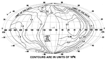
Figure 1: RAE-2 all-sky map of the galaxy at 4.70 MHz by J. C. Novaco & L. W. Brown (1978) Novaco and Brown (1978). Repreduced by permission of J. C. Novaco and the American Astronomical Society (AAS).

In addition, the FIRST Explorer can be used to image the low-frequency Sun and the evolution and propagation of coronal mass ejections (CME), which is important for our understanding of space weather and its sometimes severe consequences for vital infrastructure on Earth. It can also perform long-term studies of all the radio-planets by providing dynamic spectra of the intense low frequency radio bursts that originate in the planets’ auroral zones. Due to the ionospheric cut-off, those planetary radio emissions are, with the exception of the Jovian decametric radiation, not accessible from Earth. Similar radio emissions are most likely produced also by extra-solar planets with magnetic fields and atmospheres. With an intensity that can exceed their host star and a frequency content directly proportional to the planet’s magnetic field strength, those burst radio emissions hold a great promise as beacons for future extra-solar planet searches.

Larger space-observatories based on the enabling passive formation-flying technology, but consisting of several small satellite constellations, are being considered as the next step. These observatories will have enhanced sensitivity and resolving power to address many fundamental science objectives in radio astronomy, such as detection and observation of extra-solar planets as well as comprehensive studies of the dark ages and the epoch of re-ionisation, by observations of high red-shift $21$ cm line emissions from neutral Hydrogen, which is the only radiation believed to have survived from the period before the Universe became transparent Loeb and Zaldarriaga (2004). With suitable long integration times, FIRST Explorer can in itself gather high red-shift $21$ cm line spectra that may be able to prove the dark ages hypothesis. A no-result is also very useful since it will put limits on the maximum strength of these emissions at the lowest frequencies, which are not accessible from Earth.

The FIRST Explorer mission concept study was commissioned by the European Space Agency (ESA) Bergman et al. (2009b) and based on an idea from one of the authors, Dr Constantinos Stavrinidis, Head of the Department of Mechanical Engineering at ESA/ESTEC, to reduce formation flying mission costs. The study objective put forward by Dr Stavrinidis was to:

“Assess the potential of an innovative and valuable science mission to achieve with low cost, a ‘passive’ formation flying instrument, by allowing the formation to drift, and overcoming the need  for demanding and expensive technologies for position control systems to constantly servo the various spacecraft into tightly defined positions”.

The cost of current and previous formation flying mission designs are driven up by the need to  employ sophisticated, often optical and thereto expensive, range sensors to monitor the position and orientation of separate spacecraft to high precision; and the need to use complex active multi-axis micro thrusters on each spacecraft, to constantly servo the constellation into a defined position and orientation.

This is a challenge for a formation involving only two or three spacecraft, but as the number increases the complexities of the servo control algorithm grows exponentially and then the growing time-delays between command and control make the challenge even more difficult.

The passive formation flying concept optimises the “knowledge” of the relative positions of the spacecraft – rather than optimising control of the position of the spacecraft. More sophisticated computational modelling is used as a trade-off against less sophisticated conventional ACOS (Attitude and Orbit Control System) instrumentation using active multi-axis thrusters.

This paper examines one possible mission concept using example design criteria, and based on existing low-cost technology that has been demonstrated in space or on the ground. It is not a full mission design study and many of the system parameters require further detailed design trade-off studies, but the paper illustrates what could be achieved as an alternative to conventional science and technology demonstrator missions.

By adopting a different paradigm, where the instrument adapts to a changing environment rather than the other way round and by postulating a mission scenario in a low-drift environment, we have designed a fresh (holistic) approach to the problem. The science goals have been iterated with the mission architecture approach, to develop a mission concept that both tests the low cost passive formation flying idea, and yet still targets valuable new astronomical science results that cannot be achieved from the ground or with conventional spacecraft designs. The resulting mission design is known as the FIRST Explorer, as it explores both the novel mission technology and control concepts and points the way to larger formations that can address some of the grand science challenges open to future space-borne low frequency radio astronomy missions.

II Passive formation-flying concept and top level mission requirements

Formation-flying studies to date have required continuous minute corrections to the orbital positions of the free flying satellites in 6 degrees-of-freedom (DOF). This increases the complexity and associated risk of controlling the formation. An alternative approach is to let the formation drift slowly and only make periodic corrections, or re-formations of the constellation, or adaptation of the mission, if necessary. This technique can benefit from a dynamic and predictive metrology modelling approach to measure the relative positions in 6 DOF to well defined range uncertainties that are within the tolerances of the science model, and then add corrections to the science data to counter for the drift effects.

It so happens that a low-frequency distributed aperture radio telescope, with the spacecraft randomly distributed in a roughly spherical constellation, and with sensors based on sets of 3 orthogonal dipole antenna, can reform the image dynamically provided that the 6 DOF range and orientation information is provided to an uncertainty of between $1/100$ and $1/360$ of the observation wavelength. With a nominal $5$ MHz observing frequency (wavelength of $60$ m), this uncertainty (circa $\pm 150$ mm) would be difficult to achieve from a ranging system based on simple low-cost omni-directional radio transponders, if only the raw performance of the individual transponders were used.

However, as we will show, the uncertainty requirement can indeed be met comfortably, even for simple transponders, by fusing the raw data from three or more transponders placed on each spacecraft. That requires a multi-lateration ranging model that computes the exact range uncertainties and combines them in a co-operative way, which significantly reduces the net uncertainty of the combined data. This technology has been well developed for high-precision large-scale three-dimensional (3D) metrology in terrestrial applications. To the best of our knowledge, we are the first to have developed and adapted such a precision measurement model specifically for passive formation-flying.

The low-drift requirement was important in our choice of orbit at the second Lagrange point (L2), because the disturbances there are relatively modest. Even so, a major issue for spacecraft that are using no, or minimal active control, with conventional propulsion systems, is that they would eventually drift out of an L2 orbit, and solar pressure would tend to separate the spacecraft over time outside a reasonable 1 to 2 year mission operation envelope.

The solar radiation pressure, which at first glance seem to have a negative influence on the mission life-time, can however be taken advantage of. We have proposed a spacecraft design that passively self-stabilizes and orientates itself towards the Sun by means of solar radiation pressure alone; and which, in addition, uses credit-card sized mini solar sails, with active deployment, to maintain the formation within the mission envelope for extended periods of time. With this design concept, use of simple mission resetting thrusters on each spacecraft might be considered only as back-up the first time the concept is tested at L2.

Other key issues for the radio astronomy mission is the high demands on accurate timing and synchronization, the data communication systems ($10-14$ Mbps inter-spacecraft communication link), and the on board processing needs for the science mission; to compensate for spacecraft drift motions and correlate the science data, which computationally is a very heavy load.

The overall novelty of the proposed passive formation-flying mission concept is embodied in the combination of existing technology. For the first time brought together in a novel mission design. The key elements that are novel in their combination are:

• The use of low-cost mobile phone type transponders, for inter-spacecraft ranging and communications of science and range data, together with a combined ultra-low mass antenna for radio astronomy and inter-spacecraft ranging.

• An advanced multi-lateration position and orientation measurement data-fusion model, which improves the effective accuracy of low precision radio range sensors by up to 30 times.

• A novel spacecraft design that self-orientates using the solar radiation pressure at L2 and uses mini solar sails to keep the constellation within an overall radio astronomy mission envelope for an extended mission life.

• The use of tri-axial antennas on each daughter spacecraft enables a full $4\pi$ steradians field of view. The resolution and sensitivity of the all-sky survey will increase with mission lifetime and benefit from the slow drifts and rotations of the constellation elements.

The top-level design challenges we have encountered are discussed in more detail in the sections below, in each case studying existing technology or proven technology concepts. The major issues considered are summarized as:

• Achieving the required distributed aperture sensitivity and resolution to advance existing science, with an affordable constellation.

• Significantly improving the knowledge of the inter-spacecraft separation and orientation over what is achieved by using simple ranging techniques only.

• A radio ranging antenna/transponder and data management system compatible with the science sensor arrangements and demands.

• Orbital control of the spacecraft separation and orientation that avoids expensive 6 DOF active control, is not vulnerable to drift forces from gravity gradient and solar radiation pressure, and keeps the spacecraft stable and sun pointing.

• Efficient data linking and computational data fusion for both the science and metrology data.

III Mission Functional and Physical Architectures.

In order to have sufficient sensitivity and resolution, the FIRST Explorer science mission requires a distributed sparse antenna array. To comply with the main science objective, which technically is to simultaneously collect radio astronomy signals from the whole celestial sphere, vector antennas capable of resolving all three components of the electric field vector are required. The limitation of communication bandwidth between Earth and L2, further requires the communication of the high bandwidth radio astronomy signals between spacecraft; so that they may be combined and processed to reconstruct the full distributed telescope aperture. This in turn requires knowledge of the relative separation and orientation of the spacecraft. After the appropriate level of on board processing, the reduced astronomy data must subsequently be transmitted back to Earth, for further post-processing, distribution and analysis.

In addition to being capable of capturing the science data to meet the science objectives, the FIRST Explorer technology mission has to perform within several constraints. The spacecraft must be within range of the sensing and communicating metrology (less than $25$ km at the limit), with sufficient inter-sensor visibility for determining relative separation and orientation to the required accuracy. Solar panels must br aligned to the Sun axis within $\pm 15$ degrees. A sufficient mission duration is required to meet the science and metrology objectives (one year nominal, greater than two years preferred). Mass, power, thermal and propulsion budgets must nevertheless be consistent with a low cost mission.

Although the constellation needs to be in a stable orbit it does not need to be pointed in a particular direction to make science observations. A random volume distribution is preferred, taking account of collision avoidance and metrology and communication ranging limitations. A planar distribution must be avoided, because in free space a plane antenna array will have no means to tell what is “up” or what is “down”. A spherical rather than disc shaped distribution is also more helpful to the metrology. Both the science and the ranging metrology model objectives can benefit from changes to the relative positions of the spacecraft within the operating constraints.

In principle, spacecraft operating at L2 will experience a balance between the combined gravitational pull of the Sun and Earth, and the centripetal force associated with orbiting the Sun at that distance in one Earth year. In practice, there is a gravity gradient so that a spacecraft slightly further away will experience a lower gravitational attraction, and a higher centripetal force from the higher speed to complete an orbit of larger circumference. The net effect is an outward drift Landgraf (2007) and the formula for calculating the relative acceleration $a_{\mathrm{gg}}$, due to the gravity gradient, of two spacecraft at L2, separated by a radial distance, $D$, is

$$a_{\mathrm{gg}}=2D\frac{\mu_{\mathrm{S}}+\mu_{\mathrm{E}}}{r_{\mathrm{S}}^{3}-r_{\mathrm{E}}^{3}}$$ (1)

where $\mu_{\mathrm{S}}=1.327\times 10^{8}$ km³s^-2 and $\mu_{\mathrm{E}}=3.986\times 10^{5}$ km³s^-2 are the gravity coefficients for the Sun and Earth, respectively, and where where $r_{\mathrm{S}}=1.48\times 10^{8}$ km and $r_{\mathrm{E}}=1.5\times 10^{6}$ km are the radial distances from the Sun and Earth, respectively.

As an example: two similar spacecraft where one is $1$ km further away from the Sun will experience a relative drift of about $150$ km in a year.

Spacecraft at L2 will also experience acceleration $a_{\mathrm{SR}}$, away from the Sun due to solar radiation pressure, which may be calculated from

$$a_{\mathrm{SR}}=\frac{c_{\mathrm{R}}S}{c}\frac{r_{\mathrm{E}}^{2}}{r_{\mathrm{S}}^{2}}\frac{A_{\mathrm{SC}}}{M_{\mathrm{SC}}}$$ (2)

where $c_{\mathrm{R}}=1.6$ is the (assumed) radiation coefficient, $S=1353$ Wm^-2 is the solar constant, $c$ is the speed of light, $M_{\mathrm{SC}}$ is the spacecraft mass, and $A_{\mathrm{SC}}$ its effective area.

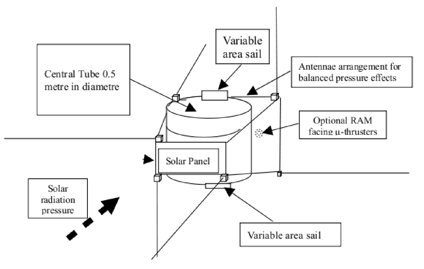
Figure 2: Daughter spacecraft architecture. The central $0.5$ m diametre tube provides a thrust tube for launch configuration and houses all electronics and the variable sail area. The sun facing (front) area is $67\times 15$ cm² and has a solar panel. The RAM face (back) area is $88\times 29$ cm². The sloping sides, top, and bottom, with $10$ degree Chamfer and $60$ cm lengths, provides self-correction to angular drift. The six monopole antennas are arranged to balance solar pressure effects. They are connected pairwise to form three orthogonal dipoles (one vector antenna). The ranging sensors, located at their tips, doubles as inter-spacecraft communication antennas.

Spacecraft relative drift from solar radiation pressure is extremely sensitive to differences in the effective area presented to the pressure. For example: two $10$ kg spacecraft with effective areas $0.314$ m² with a machined tolerance of $1$ mm could experience a difference in relative drift up to $900$ km in a year.

In theory it might be possible to select a radial distance slightly closer to the Sun and Earth where the solar radiation pressure was balanced by slightly stronger gravitational pull but natural variations in solar pressure and gravitational effects make this impractical. Some form of drift management is therefore required to meet the basic mission requirements.

A simple, robust and highly reliable method of controlling relative drift is by changing the effective area exposed to the solar radiation pressure. Because relatively small differences have significant effects over longer periods of time the changes to effective area can be quite small. The easiest form is an extending or retracting ‘sail area’ as shown in Fig. 2. Depending on the design this mini solar sail could be controlled by a space qualified ‘stepper motor’ or even possibly thermally actuated expansion and contraction. It would be very important to ensure that the effect was balanced so as not to introduce unwanted torques. A further refinement might be to effect some ‘limited steering’, by offsetting the mini sails and “tacking across the solar pressure field”, but this would need to be modelled carefully to determine feasibility and traded-off against the risks from greater complexity. A fall-back option is to put a micro thruster in the RAM face to counter the rate of drift.

This approach indicates a daughter spacecraft design similar to that in Fig. 2 with a target mass of $10$ kg. The wedge-shaped body is built around a central circular thrust tube, which can also be used to stack the spacecraft for launch and transit to L2. The one metre monopoles for LF sensing and metrology antennae deploy once the spacecraft reaches its operational orbit. The electronics are packaged within the thrust tube to give maximum radiation shielding. A $50$ W continuous power budget from a $0.1$ m² array has been estimated as detailed in Table 1.

Table 1: Power budget for daughter spacecraft

Main power consumers	Power [W]
Data processing	$5$
Timing (rubidium standard)	$10$
Metrology (inter-satellite comms.)	$12$
Mini solar sail area management	$10$
Propulsion (operated periodically)	$5$
Margin: $20$%	$8$
TOTAL	$\mathbf{50}$

Table 2: Power budget for the mother spacecraft

Main power consumers	Power [W]
Monoevre (deployment and mantanance)	$\mathbf{\leq 200}$
Operation (X-band transmitter)	$\mathbf{\leq 200}$
Metrology (mother-daughter comms.)	$5$
Timing	$5$
Data processing	$15$
Margin	$25$
TOTAL operational requirements	$\mathbf{250}$

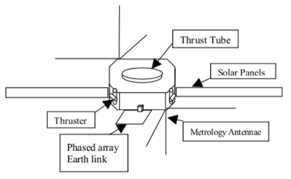
Figure 3: The hexagonal three-axis stabilised mother-spacecraft is built around a central thrust tube, $50$ cm in diameter. It has flat top panels and two solar panel wings. Active thrusters are used for full 6 DOF spacecraft control. A steerable phased array is used for communication with Earth. The antennas used for ranging and inter-spacecraft communication are of the same design as the vector antennae on the daughter spacecraft. They can be used for science, providing a $7^{\mathrm{th}}$ radio astronomy antenna or be used as a spare, if a daughter fails.

The Mother spacecraft will need to manoeuvre very precisely with 6 DOF to deploy the daughter spacecraft with negligible relative linear or angular velocity. Ideally this should vary by less than $0.1$ ${\mu}$N of thrust or torque. It will therefore have to be highly stable during these manoeuvres suggesting a highly effective 6 DOF AOCS and a significantly larger mass than the daughter spacecraft. The mother spacecraft also needs sufficient propulsion for the transit to L2 and to remain in loose formation with the daughter spacecraft once they have been deployed.

It is assumed that the mother spacecraft will be built around a 0.5 m thrust tube providing the interface to the launch separation system below and the daughter spacecraft stack above.

The most challenging task for the AOCS is the very precise control of the separation of the daughter spacecraft. This requires precise knowledge and control of the motion of the mother spacecraft at the time of each separation. A star tracker, even supplemented with sophisticated MEMS gyro arrangements, is unlikely to offer the necessary accuracy. The challenge therefore is to exploit the in-built metrology range sensor network in place for the formation-flying; in this case however the sensing will be ‘rate’ rather than ‘position’ based. This may extend the deployment phase to allow sufficient ‘settling time’ and to build up a sufficient statistical sample to achieve the necessary accuracy.

The mother spacecraft must be capable of independent navigation to L2 requiring Sun sensors and a simple star tracker. The sun sensors would need to be arranged on all potential Sun facing surfaces. The star tracker will probably be best placed on the side of the spacecraft facing away from the sun during transit to L2. For redundancy purposes, two star trackers are advisable. Miniature video cameras to observe critical manoeuvres may be considered.

Table 3: Mass budget for the FIRST Explorer spacecraft

Sub-system estimate	Mass [kg]
Electric propulsion (wet mass)	$50$
Solid chemical motor (transit)	$30$
Communications equipment	$5$
AOCS	$5$
Power generation and distribution	$15$
Timing and data processing	$5$
Structure (incl. separation system)	$45$
Margin	$40$
TOTAL Mother	$200$
Six daughters ($10$ kg each)	$60$
TOTAL All spacecraft	$260$

The propulsion system must both provide the transit to L2 and precise control the spacecraft in 6 DOF once there. Probably only electric propulsion can offer the fine control needed but it is unlikely to also have the power to achieve a rapid transit to L2. This probably needs a small solid chemical motor. For the electric propulsion one can envisage two thrusters for the $Y,Z$, pitch, roll and yaw motions and four thrusters for the $X$ motion; each thruster is assumed to be capable of $2$ mN in the normal thrust mode and less than $0.1$ ${\mu}$N in the differential mode. Rule of thumb calculations indicate that a $200$ kg mother spacecraft and six $10$ kg daughters, can move the kilometre or so needed between initial deployment positions in 4 or 5 hours before settling time. It would therefore appear reasonable to plan the full six spacecraft deployment sequence over 6 to 12 days.

The mother spacecraft data processing will at a minimum need to combine the science and range metrology data streams from the daughter spacecraft and re-transmit a pre-processed product to Earth. Preferably, the majority of science data fusion and metrology data processing would take place on the mother spacecraft with only the final processed product being relayed to earth. Even after processing there will be a reasonable volume of data to be transmitted back to Earth and there may be instances where raw data is required for analysis or anomaly investigation. A trade off study is needed to establish the best balance between mother spacecraft processing power and the volume of data for Earth transmission. At this stage we propose an X-band link, capable of several Mbps data rate, operating through a flat plate phased array which can be deployed from the side of the Mother spacecraft after separation from the launch vehicle. Some rudimentary mechanical steering may also be needed.

The estimated power budget for the mother-spacecraft is based on realistic assumptions and detailed in Table 2, which in round terms suggests the need for $250$ W of BOL installed power, which ould be met with two $2\times 0.25$ m² solar panels. These considerations suggest a mother spacecraft design concept as shown in Fig. 3.

Given the relatively low propellant requirements with electric propulsion, a total mass budget of $260$ kg for the FIRST Explorer mission has been estimated, as detailed in Table‘3 It is considered to be challenging but not unreasonable (based on a $20$% margin).

IV Communications and ranging system

The overall system aims to fulfil three objectives: transmission of the science data, transmission of signal and control data, and ranging. Within the approach that we have chosen, RF power, system complexity, operating-range limits and range accuracy are issues that have conflicting requirements. The principal technologies that we have considered are IEEE 802.11 (WiMAX) IEE (2007), which is an Orthogonal Frequency Division Multiple Access (OFDMA) $20$ MHz bandwidth system capable of transmission rates of up to $54$ Mbps and Wideband Code Division Multiple Access (WCDMA), which is a $5$ MHz bandwidth system used for mobile communications with data rates of up to $384$kbps UMT (2005).

In the ideal configuration, the separation of the mother and daughter satellites will be comparable and in the region of $5-15$ km. The optimum configuration for communication is a star network, as used in mobile communications and wireless networks, with the mother as the controller. However, if the satellites drift into a non-ideal configuration, the separation between all satellites and their near neighbours may be close enough to permit communication but may exceed the range limits for a star network. An alternative data path is required in case the direct link to the mother spacecraft is lost. The required configuration will be a peer-to-peer or ad-hoc network, similar to mobile sensor network architectures, where one of the daughter satellites acts as the controller, and the data is passed back to the mother spacecraft in multiple hops.

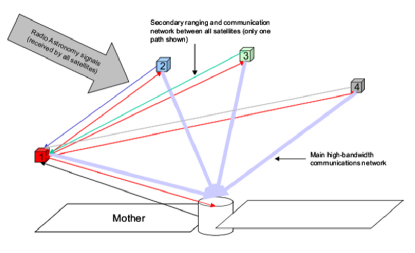
Figure 4: Communications and ranging showing the primary and secondary networks. Two-way communication between ‘Daughter 1’ and the other satellites provides ranging and data communications.

As illustrated in Fig. 4, the proposed communications architecture will comprise a main, high-bandwidth star network centred on the mother satellite and a secondary reconfigurable network between all of the satellites. The secondary network also provides both communication and ranging functions.

Within the constellation, the majority of the communication bandwidth will be used to transmit the science data back to the mother satellite. The science data from each of the satellites requires a capability of circa $14$ Mbps to support an acquisition bandwidth of $100$ kHz.

As all the spacecraft drift they will have different rotation rates and relative orientations so it is essential that the antennas radiate with a wide field pattern to maintain communication. The path loss can be calculated using the Friis equation Friis (1946), which can be written

$$P_{\mathrm{r}}=P_{\mathrm{t}}G_{\mathrm{t}}(\theta_{t},\varphi_{t})G_{\mathrm{r}}(\theta_{r},\varphi_{r})\left(\frac{c|\mathbf{\epsilon}_{r}\cdot\mathbf{\epsilon}_{t}^{\ast}|}{4\pi fD}\right)^{2}\,,$$ (3)

where $P_{\mathrm{t}}$ and $P_{\mathrm{r}}$ are the transmitted and received powers, respectively, $G_{\mathrm{t}}$ and $G_{\mathrm{r}}$ the corresponding antenna gain patterns, $f$ is the frequency, $c$ is the speed of light, and $D$ the separation distance. Polarisation losses are accounted for by means of the absolute value squared of the scalar product between the antenna polarisation (unit) vectors, $\mathbf{\epsilon}_{\mathrm{t}}$ and $\mathbf{\epsilon}_{\mathrm{r}}$. These are in general complex valued but becomes real valued for linearly polarised antennas.

For the calculations we have assumed an antenna gain of $1.5$ dB, typical of a linearly polarised electric dipole antenna, and average orientation and polarisation penalties of $3$ dB. At $10$ km range and an operating frequency of $2$ GHz we anticipate an average path loss of $121$ dB between any pair of antennas. In practice, as there are several antennas to allow for the relative orientations of the satellites it will be possible to make use of receive (and transmit) diversity to increase the system sensitivity.

Power, range and data throughput are intimately connected. Previous work by Mahasukhon et. al. Mahasukhon et al. (2007) showed that the popular IEEE 802.11 WLAN standards, require a Signal-to-Noise Ratio (SNR) of about $22$ dB to achieve $54$ Mbps operation and $3$ dB to achieve 6 Mbps operation. Although the maximum bit rate is $54$ Mb/s, the saturation throughput depended on the exact implementation of the standard. For a channel bit error rate (BER) of $10^{-5}$ the saturation throughput is $23.2$ Mbps for IEEE 802.11a and $9.7$ Mb/s for IEEE 802.11g. The inference is that, the Media Access Control (MAC) layer and operating frequency will need to be tailored for this application to achieve the required performance and range.

A noise power of $-100.8$ dBm has been calculated assuming a $20$ MHz bandwidth and a receiver temperature $T_{\mathrm{rec}}=300$ K. The limiting range can be found for any frequency and SNR by rearranging the Friis equation, Eq. (3), and using the noise threshold levels calculated from Mahasukhon et al. (2007). An additional factor, $G_{\mathrm{d}}$, which accounts for the diversity gain, has been included in the equations because each satellite uses several antennas and these signals can be combined constructively to increase the sensitivity. In this analysis the average value of the diversity gain has been conservatively set to $G_{\mathrm{d}}=2$ ($3$ dB). The range limit can then be calculated from

$$D_{\mathrm{lim}}=\frac{c|\mathbf{\epsilon}_{r}\cdot\mathbf{\epsilon}_{t}^{\ast}|^{2}}{4\pi f}\sqrt{\frac{P_{t}\langle G_{\mathrm{t}}\rangle\langle G_{\mathrm{r}}\rangle\langle G_{\mathrm{d}}\rangle}{k_{\mathrm{B}}T_{\mathrm{rec}}n_{\mathrm{SNR}}\Delta f}}\,,$$ (4)

where $k_{\mathrm{B}}$ is the Boltzmann constant, $\Delta f$ is the bandwidth, $\langle G_{\mathrm{t}}\rangle$ and $\langle G_{\mathrm{r}}\rangle$ are the average values for the antenna gains (isotropic, 0 dBi) and $n_{\mathrm{SNR}}$ is the signal-to-noise ratio (SNR) required to support a specific data rate. The polarisation factor $|\mathbf{\epsilon}_{r}\cdot\mathbf{\epsilon}_{t}^{\ast}|$ has been set to $1/\sqrt{2}$, which corresponds to an average misalignment between the polarisation vectors of $45$ degrees. The results, shown in Fig. 5, infer that a system based on IEEE 802.11 coding standards will meet the bandwidth and range requirements.

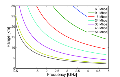
Figure 5: Data rate range and operating frequency limits for WLAN. The SNR values ($n_{\mathrm{SMR}}$) employed, from $6$ Mbps (top curve) to $54$ Mbps (bottom curve), were, $3.3,6.4,10,13,17,21$, and $22.4$.

The ranging system provides the data for the multi-lateration model to determine the relative positions and orientations of the spacecraft. The two main ranging options are to use an independent, self-contained solution, or to use a cooperative approach. The limitation of the self-contained radar approach is that the returned power is inversely proportional to the fourth power of the separation between the source and target, limiting the operating range. For this reason a cooperative, communications based approach has been adopted. Each two-way communication link provides ranging information so the desired outcome is to maintain communication links between all or as many of the satellites as possible. The number of two-way links $N_{\mathrm{2way}}$ can be calculated from the number of satellites $N$ as $N_{\mathrm{2way}}=N(N-1)/2$.

The system will require many separate communication links. Code Division Multiple Access (CDMA) techniques use orthogonal codes to provide diversity and hence allow the re-use of the carrier frequency. A code length of 256 bits will provide 64 orthogonal code channels.

In ground-based systems, the location accuracy of mobile transmitters within a cellular radio system may be limited by non line-of-sight errors Shanmugam et al. (2005) to about $20$ metres and this can be considerably improved using interferometric techniques to give accuracies of $0.6$ m Kusy et al. (2007). In a space environment, multi-path fading signals will be much less of an issue as the separation and cross-section of the satellites is small. There will be some interaction between the antennas and the spacecraft that will require calibration and correction to achieve the required accuracy.

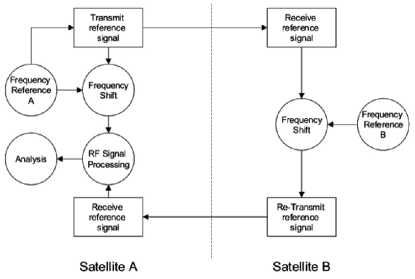
Figure 6: Cooperative ranging by re-transmitting a frequency-shifted signal.

The inference of these studies is that the timing accuracy achievable through the MAC layer is insufficient to provide the required ranging accuracy but will ensure that more accurate methods do not suffer from cyclic errors.

Several options are available for cooperative ranging: time of flight for a re-transmitted signals gives a resolution that is inversely proportional to the signal bandwidth $\Delta R\approx c/3\Delta f$.

Edge timing of a Time-Domain Diversity communications system with a bandwidth of $20$ MHz would correspond to an accuracy of $5$ m, which is insufficient for the requirement. Using a short RF pulse, rather than the communications system, could improve the accuracy by an order of magnitude but co-operative management of the ranging function throughout the constellation would be more difficult as only one satellite transponder could obtain range information at a time.

The relative motion of the satellites must be taken into account in any implementation. As the distance between the two craft separates the phase of the received and demodulated RF signal will rotate through $2\pi$ for every wavelength of separation. In a typical system, the phase or frequency of the Voltage Controlled oscillator will track these variations. If this information can be accessed within the RF chip/chip set it will correspond to an uncertainty of circa $\pm 30$ mm for a $2$ GHz carrier, assuming a phase stability of $\pm 1.25$ radians.

Consider the simple implementation shown in Fig. 6, where a received signal is frequency shifted and retransmitted. As the reference oscillators within each of the satellites are independent, the signal processing system must be designed to separate frequency shift, velocity components, and $2\pi$ ambiguities. Uncertainties in satellite time-transfer have been studied in detail Parker and Zhang (2005), and the expected uncertainty of the transponder path-delay calibration is expected to be less than $1$ ns Whibberley (2009), giving an overall uncertainty better than $\pm 150$ mm.

In summary, a communication system based on COTS hardware with additional components is expected to have the capability of providing the required data handling ($14$ Mbps per satellite) at circa $5-25$ km separation and a ranging uncertainty of less than $\pm 150$ mm, as required by the proposed application.

V Fusing range measurements to determine formation configuration geometry

The basis of the FIRST Explorer passive formation-flying concept is that of allowing movement between spacecraft but with the relative locations and orientations of the spacecraft determined to precise limits from range data. A mathematical (multi-lateration) model and associated software have been developed to analyse various designs and to predict the uncertainty in configuration geometry from range and time measurements.

The model assumes a fixed number of spacecraft undergoing approximately constant linear and angular motion where each spacecraft has a fixed number of range transponders or targets at known positions. At any given time, six parameters are required to determine the position of a spacecraft: three to determine location and three to determine orientation. Six constraints need to be applied to fix the frame of reference of the overall constellation of spacecraft. For spacecraft undergoing constant linear and angular motion, twelve parameters are required per spacecraft, six to determine an initial position, three to specify the direction and speed of the linear motion, two to determine the axis of rotation and one to specify the speed of angular rotation. Nine constraints need to be applied, six to fix a frame of reference and three to specify the initial linear motion applying to the constellation as a whole.

In practice, the behaviour of the range transponder will depend on the angles of the line-of-sight. The model assumes that this behaviour can be specified in terms of one or more direction vectors and acceptance angles associated with the target position. If the angles between line-of-sight joining two targets are smaller than the acceptance angles at each of the targets, then the associated range measurement is admissible. At any given time, the acceptance angles associated with a range measurement between any pair of targets can be estimated from the parameters describing the motion of the constellation.

It is assumed that each measured range value estimates the distance between a pair of targets at a given time, one target on one spacecraft, one on another. To each range measurement is associated a time and two indices specifying the two targets. Uncertainties are also associated with the range measurements, based on a characterisation of the transponders and can be used to provide weights for the measurements. For example, each range measurement can be weighted according to the angles of incidence, with the maximal weight equal to one if the line of sight is aligned exactly with the corresponding direction vectors.

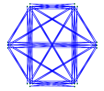
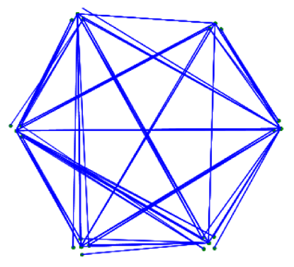
Figure 7: Admissible range measurements associated with six targets on each of six satellites in an initial position (top panel) and after drifting (bottom panel).

Given motion parameters, contained in the vector $\mathbf{a}(t)$, specifying the motion of the constellation, at any given time $t$, the distance $D_{nm}=D_{nm}(\mathbf{a}(t))$ between any two targets, $n$ and $m$, can be predicted. Given range measurements, $d_{nm}$, estimates of the motion parameters, $\mathbf{a}$ can be determined by matching the model predictions to the actual observations in the least squares sense. The uncertainties associated with the range measurements can be propagated through to those associated with the fitted parameters using standard methods Forbes (2009a, b); Peggs et al. (2009)

A set of simulation tools has been implemented in Matlab. The software is completely flexible with respect to the number and configuration of spacecraft, the number, location and acceptance behaviour of the targets (range transponders on the spacecraft), and the number and timings of the range measurements; all that is required is that each range measurement has an associated time and indices specifying the targets involved.

In terms of design considerations for the FIRST Explorer concept, the number of spacecraft has been fixed at six, with up to six transponders on each daughter spacecraft. A primary concern is having enough range measurements to provide an accurate assessment of the constellation geometry for almost arbitrary motion of the spacecraft. A balance has to be made between

• maximising the number of admissible range measurements for a particular, ideal constellation geometry, and

• making sure that if the constellation drifts from its optimal shape there are sufficient range measurements available to meet the accuracy requirements.

It is assumed that any constellation will suffer from drift and that over a long period there can be no guarantee that a constellation will match a preferred geometry. Furthermore, the slow rotation of each spacecraft about its main axis cannot be ruled out. This means that a transponder design that depends significantly on a particular constellation geometry runs the risk of degraded performance as time progresses. The simulations discussed below make the following assumptions: the centre of gravity of each spacecraft drifts linearly a few metres over the time scale of a few days, each spacecraft rotates about an axis a few times per day, the rates of rotation about the axes are different. The simulations reported below also assume that each spacecraft maintains at least a rough alignment with the sun (up to $30$ degrees misalignment). The most significant assumptions above relate to rotation since they are used to make sure the constellation geometry does not become stuck in a static case in which there are very few admissible range measurements. The conclusions below hold for different rates of drift and rotation if the time scales are adjusted appropriately.

The transponders have the following acceptance behaviour consistent with a radio transponder that is not fully omni-directional but has preferred gain patterns of sensitivity. Each transponder is associated with a direction vector. If a line of sight makes an angle of between $60$ and $120$ degrees with the direction vector, the range measurement is admissible for that transponder. Thus, a range measurement is admissible for a target if it makes angles of less than $30$ degrees with the plane orthogonal to the direction vector; this is termed a “doughnut” acceptance profile. Additionally, a range measurement is admissible for that target if the line of sight makes angles of less than $30$ degrees with the direction vector, giving a “one-sided cone” acceptance profile. A range measurement is admissible if it satisfies at least one of the acceptance criteria at each end.

The advantage of the design of transponder is that if the direction vector is not aligned with the axis of rotation of the spacecraft, the doughnut acceptance region sweeps through the whole of 3D space in one rotation so that the transponder has a chance to see all others in the constellation. The different rates of rotation are used to guarantee that the rotations are not locked together making some, possibly many, of the range measurements permanently inadmissible.

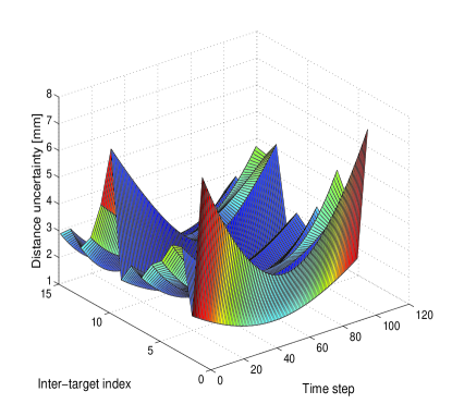
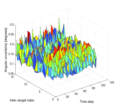
Figure 8: Uncertainties associated with the separation distances (left panel) and angles (right panel) between spacecraft centres of gravity at 101 time steps. There are six spacecraft and 15 inter-spacecraft distances.

The following simulations involve six spacecraft randomly situated in an oblate sphere of equatorial diameter $5$ km and polar diameter $3$ km. Each suffers constant linear drift in a random direction and constant rotation about a random axis aligned to within $30$ degrees of a fixed axis (pointing to the sun). Each satellite has six transponders situated at the centre of the faces of a cube of side $3$ m. The direction vectors associated with the transmitter/receivers are aligned with the vector joining the centre of the cube to the corresponding faces.

The simulation calculates,

• the uncertainties associated with the distances between the centres of gravity for each pair of spacecraft at each time step,

• the uncertainties associated with the angles between fixed vectors for each pair of spacecraft at each time step, and

• the uncertainties associated with the parameters specifying the constant motion of the constellations.

The measurement uncertainty for the determination of the range between any two targets, with the radio range transponder discussed in Section 4 above, is taken to be $\pm 150$ mm.

The simulations show that the ratio of admissible range measurements to all possible range measurements is low, of the order of $5$%. However, as shown by the illustrations in Fig. 7, the admissibility profile can change as the formation evolves with time. The simulation has shown that For 100 time steps, there are typically over 5000 admissible range measurements.

The evaluated uncertainties associated with the inter-spacecraft distances, as shown in the left panel of Fig. 8, are of the order of better than $\pm 10$ mm at all time steps and the uncertainties associated with the angles, as shown in the right panel of Fig. 8, are less than $\pm 0.5$ degrees.

The uncertainties for the inter-spacecraft distances have a typically U-shaped behaviour with respect to time. The distances for middle time periods use information from the past and future, while initial and final time periods can only use future or past measurements, respectively. The uncertainties associated with the angles are much more sensitive to which inter-target pairs are associated with admissible range measurements and hence vary from time step to time step as the admissibility pattern changes. Integrating over a long time or taking measurements at a greater rate would reduce the uncertainties further.

VI The science mission requirements

The Universe at very low frequencies is virtually unexplored, as illustrated in Fig. 1 by the very sparse all-sky map at 4.70 MHz. It was constructed from observations made by the Radio Astronomy Explorer 2 (RAE-2) Alexander et al. (1975) and published in 1978 by Novaco & Brown Novaco and Brown (1978). It is still the best picture we have of the Universe at this very low frequency. The main reason for our evident lack of knowledge is the Earth’s ionospheric plasma, which effectively blocks out radio frequencies below the ionospheric cut-off, about $10$ MHz, and makes observations below $\sim 30$ MHz very difficult. Therefore, astronomical observations at low frequencies require a space borne radio telescope.

The FIRST Explorer is aimed to be such a telescope. Its primary science objective is to provide a new all-sky survey at very low radio frequencies with improved sensitivity and an angular resolution better than $1$ degree. A secondary objective is to observe radio sources in the solar system, such as the low-frequency Sun and non-thermal planetary radio emissions. Those emissions will in any case interfere with the all-sky survey and therefore needs careful monitoring. The secondary objective thereby complements the primary one. A third objective is to try to detect high red shift 21 cm Hydrogen line emissions Loeb and Zaldarriaga (2004), or at least put limits on the maximum strength of the low-frequency part of this radiation, which should now be in the $9$ –$200$ MHz range. It is the only known way to probe the “dark ages” from recombination to reionisation, a transition period when the first galaxies were formed and the Universe went from being completely opaque (the dark ages) to becoming transparent when the first stars formed and were able to ionise the interstellar medium. A detection could prove the dark ages hypothesis, which would be major step in observational cosmology.

Low-frequency radio astronomy tends to be very suitable for a space mission. As one first might think, it does not require a huge dish antenna to be deployed or constructed in orbit. Instead, and as we will show, a relatively modest array of simple dipole antennas can be used. The physical reason for this is the effective collecting area of the dipole, which is proportional to the wavelength squared. To increase the area, and hence the sensitivity, one just adds more dipoles to form an antenna array; although, a space array requires several spacecraft flying in formation.

The sensitivity increases linearly with the number of spacecraft so even though the RAE-2 used a 229 meter long travelling-wave V-antenna as well as a 37 meter long dipole Alexander et al. (1975), a space array would be a considerable step forward. The largest improvement, however, would be if the antenna signals could be combined and used to perform radio interferometry. With suitable separation distances that would dramatically improve the angular resolution of the observations.

The science cases for space borne low-frequency radio astronomy are well established Kassim and Weiler (1990) and have been worked upon since the last attempt by RAE-2 and free-flying as well as lunar-based observatories have been proposed. The Astronomical Low-Frequency Array (ALFA) Jones et al. (2000) and the Solar Imaging Radio Array (SIRA) MacDowall et al. (2005), are two noteworthy NASA studies of the free-flying concept, none of which became realised. Sadly, the high cost, associated with the complex technologies traditionally considered necessary for precision formation-flying, has always been an Achilles heel for previously proposed low-frequency space arrays; not to mention the cost of a deploying an antenna array on the Moon. The FIRST Explorer, on the other hand, uses passive formation flying, which for the first time can make a low-frequency space observatory affordable.

The slowly drifting and rotating spacecraft put new requirements on the science payload, i.e., the radio astronomical antennas. The drift is actually not a problem but an advantage. It allows sampling of more baselines and hence gives better coverage than would a traditional formation, where the spacecraft are forced to stay put at locked positions. The rotations can be taken care of by using a vector antenna, consisting of three orthogonal electric dipole antennas, which allows sampling of the full three-dimensional electric vector field, $\mathbf{E}(\mathbf{(}x)_{n},t)$, at the satellites’ positions $\mathbf{x}_{n}$ and time $t$. The electric field vector $\mathbf{E}_{n}(t)=\mathbf{E}(\mathbf{x}_{n},t)$ picked up by the antenna on the $n^{\mathrm{th}}$ satellite is low-pass filtered, digitised, bandpass filtered and converted to base-band by the radio receiver. It is represented as a time series of complex vectors.

Since we are only considering astronomical source the intensities $I_{n}=\langle\mathbf{E}_{n}\cdot\mathbf{E}_{n}^{\ast}\rangle$ (brackets mean time average) are equal on every spacecraft. Because $I_{n}$ is a scalar it is invariant under rotations Carozzi et al. (2000), also those performed by spacecraft. In terms of intensity, a receiving vector antenna is therefore isotropic.

However, intensity measurements are not sufficient to perform interferometry. We must also be able to measure the time differences between the field vectors registered on different spacecraft. Let $\mathbf{E}_{n}=\mathbf{E}_{0}\exp(\mathrm{i}\Phi_{n})$, where $\Phi_{n}$ is the phase. The operation $\mathbf{E}_{n}\cdot\mathbf{E}_{n}^{\ast}=\mathbf{E}_{0}\cdot\mathbf{E}_{0}^{\ast}$ makes the phase information vanish but if we instead take the scalar product without complex conjugation (denoted by superscript $\ast$) we find that the operation $\mathbf{E}_{n}\cdot\mathbf{E}_{n}=\mathbf{E}_{0}\cdot\mathbf{E}_{0}\exp(\mathrm{i}2\Phi_{n})$ preserves the phase, which can then be recovered, since $\Phi_{n}=\mathrm{Arg}[\mathbf{E}_{n}\cdot\mathbf{E}_{n}]/2$. The complex scalar $\mathbf{E}_{n}\cdot\mathbf{E}_{n}$ is also rotation invariant and in that sense the phase $\Phi_{n}$ can be said to be absolute.

If we instead would use the phase from only one $\mathbf{E}$-field component that would not have been the case since the component values are dependent on the coordinate system. Therefore, rigorous tracking of the spacecraft attitude, and continuous compensation for their rotations in software, would have been required.

In addition to being rotation invariants, using the Maxwell equations, it is not difficult to show that E·E* as well as E·E obey conservation laws and are thus true physical observables.

Having established that vector antennas can be used as isotropic and phase preserving astronomy sensors it is clear that the performance of the FIRST Explorer array to a very large extent will depend on precise time and precision range measurements.

For simplicity, consider a two-element interferometer with antennas separated by a distance $D$ and receiving a radio pulse from an angle $\alpha$ with respect to the baseline between the two antennas. As illusttraded in Fig. 9, the radio pulse, which travels with the speed of light, $c$, hits the first antenna at time $t=0$. It will hit the second antenna at a later time $t$. Using basic trigonometry we obtain the formula

$$ct=D\cos\alpha\,.$$ (5)

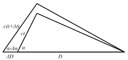
Figure 9: Geometry of a two-element interferometer of length $D$, receiving a radio wave from an angle $\alpha$. The time and distance errors, $\Delta D$ and $\Delta t$, respectively, give rise to a pointing error $\Delta\alpha$.

Hence, by measuring time $t$ and separation distance $D$ we can calculate the direction to the source. Or vice versa, by using time delays or changing the separation distance we can point the interferometer in different directions. In reality, time and distance can never be determined exactly and the errors will result in an uncertainty in the pointing accuracy, $\Delta\alpha$, which is the angular resolution of the interferometer.

Let $t\rightarrow t+\Delta t$ and $D\rightarrow D+\Delta D$, where $\Delta t$ denote the timing error and $\Delta D$ the error in distance, as shown in Fig. 9 Trigonometry yields

$$c(t+\Delta t)=D\cos\alpha+c\Delta t=(D+\Delta D)\cos(\alpha-\Delta\alpha)\,.$$ (6)

Note that $\Delta t>0$ gives $\Delta\alpha<0$ but $\Delta D>0$ gives $\Delta\alpha>0$, which means that the errors may cancel each other. To investigate if they do we assume the errors to be independent and Gaussian with zero mean values. Squaring Eq. (6) and taking the time average yields

$$\langle(D\cos\alpha+c\Delta t)^{2}\rangle=D^{2}\cos^{2}\alpha+c^{2}\langle\Delta t^{2}\rangle$$ (7)

$$= \langle(D+\Delta D)^{2}\cos^{2}(\alpha-\Delta\alpha)\rangle$$

$$\approx D^{2}\cos^{2}\alpha+\langle\Delta D^{2}\rangle\cos^{2}\alpha-D^{2}\cos(2\alpha)\langle\Delta\alpha^{2}\rangle\,,$$

where in the last step we have used the Maclaurin series expansions of $\cos\Delta\alpha$ and $\sin\Delta\alpha$. Thus, on average, the standard deviations of the time and distance errors help to reduce the standard deviation in pointing accuracy.

$$\langle\Delta D^{2}\rangle\cos^{2}\alpha-c^{2}\langle\Delta t^{2}\rangle\approx D^{2}\cos(2\alpha)\langle\Delta\alpha^{2}\rangle\,,$$ (8)

A space array must be able to handle radio waves coming from all directions. Assuming that the sources are uniformly distributed we integrate Eq. (8) from $\alpha=0$ to $\alpha=2\pi$, which yields $\langle\Delta D^{2}\rangle\approx 2c^{2}\langle\Delta t^{2}\rangle$. In other words, to minimise the average standard deviation of the pointing accuracy, the standard deviations of the time and distance errors, $\sigma_{\Delta t}$ and $\sigma_{\Delta D}$ respectively, should be chosen such that $\sigma_{\Delta D}=\sqrt{2}c\sigma_{\Delta t}$. By this choice, the angular dependency in Eq. (8) actually vanishes, instead

$$\langle\Delta\alpha^{2}\rangle\approx\frac{\langle\Delta D^{2}\rangle}{2D^{2}}=\frac{c^{2}\langle\Delta t^{2}\rangle}{D^{2}}\,.$$ (9)

In Section V it was shown that an inter-spacecraft distance uncertainty of $\pm 10$ mm was possible to achieve. To match that error, as to minimise the average pointing uncertainty, would require a time uncertainty of $\pm 24$ ps. For a $1000$ m baseline the corresponding pointing uncertainty is only $\pm 2$ arc-seconds, well below the required $1$ degree resolution. While it has shown possible to achieve such small time uncertainties in ground based antenna arrays, using a common reference frequency and adjusting the phase of the receivers by using GPS clocks Johansson (2009), that approach is impractical for a space observatory, which aims to be omni-directional. Because, to make use of high time precision, one has to delay the signals by fractions of the sampling period, which is about $10$ ns for a state-of-the-art $100$ Msps $16$ bit ADC (analogue-to-digital converter). Although it is possible to implement several fractional sample delays (FSD), their number is finite, which results in a telescope having only a finite number of looking directions. However, this approach may be of interest for observation of specific radio sources, such as auroral kilometric radiation (AKR) generation regions, with ultra-high angular resolution.

Given the $1$ degree requirement and the $\pm 10$ mm distance uncertainty it is clear that the required time uncertainty can be reduced significantly. Setting $\Delta D=0$ in Eq. (6), squaring, time averaging and integrating over $\alpha$ yields

$$\langle\Delta\alpha^{2}\rangle\approx\frac{2c^{2}\langle\Delta t^{2}\rangle}{D^{2}}\,.$$ (10)

Based on the assumed sampling period we should at least have $\sigma_{\Delta t}=\sqrt{\langle\Delta t^{2}\rangle}\leq 10$ ns. Eq. (10) then gives a separation distance $D\geq 240$ m for a $1$ degree angular resolution.

The above discussion is valid for observations times during which the drift of the clocks can be neglected. For long term observations the $\langle\Delta t\rangle=0$ assumption is no longer true. Assuming linear drift rate $k$ we let $\Delta t=kt+\epsilon(t)$ where $\epsilon(t)$ is the previously assumed Gaussian error. The variance of the time error at time $t$ is then $\langle\Delta t\rangle=kt/2$. In order to perform interferometry the accumulated time error must be less than one period of the observation frequency, or the fringes will be smeared out. Hence, $\langle\Delta t\rangle=k\Delta T/2\leq 1/f_{\mathrm{obs}}$ is required. Here $\Delta T$ is the observation (integration) period. For example, observation at $5$ MHz during one year requires a drift rate $k\leq 1.5\times 10^{-13}$, which is possible using a rubidium standard. For instance, the Rubidium standard developed for the Galileo satellites has a time deviation of $10$ ps after $100$ seconds and $1$ ns after $100000$ seconds, which corresponds to a drift rate about $10^{-14}$. To keep the angular resolution below $1$ degree during the one year period requires a separation distance $D\geq 4.8$ km for $5$ MHz observation frequency and $k=1.5\times 10^{-13}$.

As can be understood by this analysis, the observations should begin with the high frequencies, when the spacecraft are close together and the accumulated time error is small. As the spacecraft drift apart one should observe at lower frequencies and take advantage of the increased separation distance to keep the resolution within specification.

In reality the FIRST Explorer will consist of more than two spacecraft. The above analysis is therefore not all conclusive. However, it shows that the concept works and the reasonable numbers so obtained have been used in the first iteration of the design study. The design parameters for FIRST Explorer are summarised in Table 4.

Table 4: Design parameters for FIRST Explorer

Parameter	Symbol	Range
Frequency	$f$	$0.5$ – $50$ MHz
Distance	D	$0.5$ – $30$ km
Resolution	$\Delta\alpha$	$\leq 1$ degree
Time error	$\Delta t$	$\leq 1$ ns in $24$ hours
Range accuracy	$\Delta D$	$\leq 150$ mm at all times
Sensitivity	$S_{\mathrm{min}}$	$\leq 10$ Jy in $1$ hour
Bandwidth	$\Delta f$	$100$ kHz
Integration time	$\Delta T$	$1$ s – $1$ year

To determine the required number of spacecraft we must specify a sensitivity requirement. Sensitivity is measured in Jansky [Jy]. It is a non-SI unit of electromagnetic energy flux density. In SI units $1$ Jy = $10^{-26}$Wm^-2Hz^-1. From this definition one realises that the amount of collected energy depends on the collecting area of the antenna, frequency bandwidth, and observation time. The sensitivity could in principle be lowered indefinitely by time integration but as shown above that is not the case due to the accumulated time error.

Intermittent bursts of low-frequency radiation are common in the solar system and will disturb the low-frequency survey if those emissions are not handled properly. The FIRST Explorer must be able to blink to avoid glare and blinking requires action in a relatively short time period. Specifically, using a $\Delta f=100$ kHz frequency bandwidth, the telescope shall be able to detect all non-thermal planetary radio emission after $\Delta T=1$ hour integration time and strong emissions from the Sun, Jupiter, Earth, and Saturn within $1$ second. Solar type III burst and AKR from Earth are the strongest, in the order of $10^{8}$ Jy. The Jovian radio emissions are about $10^{6}$ Jy, while those from Saturn circa $10^{4}$ Jy. Then follows Uranus and Neptune, about $100$ Jy and $10$ Jy, respectively.

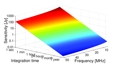
Figure 10: Sensitivity of the FIRST Explorer with six spacecraft as a function of integration time and observation frequency.

For any receiver system, the minimum energy flux density that can be detected is given by

$$S_{\mathrm{min}}=\frac{S_{\mathrm{sys}}}{\sqrt{\Delta f\Delta T}}$$ (11)

where $S_{\mathrm{sys}}=S_{\mathrm{rec}}+S_{\mathrm{sky}}$. The sky is very bright at low frequencies. It has a peak about $3.6$ MHz where the corresponding sky-noise brightness temperature, $T_{\mathrm{sky}}$, reaches $T_{\mathrm{max}}=10^{6}$ K. We can therefore disregard any receiver noise and set $S_{\mathrm{sys}}=S_{\mathrm{sky}}$ in Eq. (11). For a short dipole antenna $S_{\mathrm{sky}}=2k_{\mathrm{B}}T_{\mathrm{sky}}/A_{\mathrm{dipole}}$ so that

$$S_{\mathrm{min}}=\frac{2k_{\mathrm{B}}T_{\mathrm{sky}}}{\sqrt{\Delta f\Delta T}A_{\mathrm{dipole}}}\,.$$ (12)

The effective area of a (Hertzian) dipole is $A_{\mathrm{dipole}}=3\lambda^{2}/8\pi$ but between $1$ MHz and $100$ MHz, $T_{\mathrm{sky}}$ is empirically found to be proportional to $\lambda^{2.55}$ [Cane 1978], i.e., $T_{\mathrm{sky}}=T_{\mathrm{max}}(\lambda/\lambda_{\mathrm{max}})^{2.55}$, with $\lambda_{\mathrm{max}}=83$ m. Hence $S_{\mathrm{min}}$ will vary as $\lambda^{0.55}$ in this frequency range. The FIRST Explorer formation will consist of $N$ spacecraft where each spacecraft has a vector antenna. The dipole area in Eq. (12) must therefore be replaced by the corresponding expression for an $N$ element array of vector antennas, which we take as $A_{\mathrm{FIRST}}=3NA_{\mathrm{dipole}}$. The factor $3$ comes from the assumption that the radiation is isotropic. Effectively there are three $N$ element dipole arrays.

Substituting in Eq. (12) we arrive at the following formula

$$S_{\mathrm{min}}=\frac{16k_{\mathrm{B}}T_{\mathrm{max}}}{9N\sqrt{\Delta f\Delta T}}\frac{\lambda^{0.55}}{\lambda_{\mathrm{max}}^{2.55}}$$ (13)

The analysis has shown that six spacecraft are sufficient to fulfil the stipulated sensitivity requirement. In Fig. 10, we have plotted the sensitivity for frequencies, $f=c/\lambda$, between $5$ MHz and $50$ MHz and integration times, $\Delta T$, between $1$ second and $1$ year, with $N=6$ spacecraft and $\Delta f=100$ kHz bandwidth. As can be seen, the sensitivity has a quite flat frequency responce. For $1$ second observations the sensitivity is in the $140-490$ Jy range and for $1$ hour observation in the $2-8$ Jy range. for very long observations, $1$ – $2$ years, the sensitivity drops to below $90$ mJy ($f=5$ MHz, $\Delta T=1$ year).

VII Discussion and Conclusion

The overall conclusions from the FIRST Explorer mission concept study are that

• FIRST Explorer can operate as a distributed aperture low-frequency radio telescope with $1$ mother and $6$ daughter spacecraft with average separation distances ranging from $5$ – $30$ km in the limit, and the science objectives will actively benefit from the daughters being allowed to drift slowly apart in position and orientation, in an L2 or similar stable orbit.

• A low cost radio frequency range transponder can use adapted COTS mobile phone technologies, and provide inter-spacecraft ranging to circa $\pm 150$ mm uncertainty. In addition, the transponders can double up as the inter-spacecraft data communications system.

• Using a metrology model developed for this study, the signals from $6$ range transponders on each of the $7$ spacecraft can dynamically monitor the formation’s mutual separations and orientations in 6 DOF; enhancing the basic transponder sensitivity by at least $15$ times to $\sim\pm 10$ mm. This provides the ability to optimally process the science signals from the distributed aperture array, operating at frequencies between $500$ kHz and $50$ MHz, and achieve the required sensitivity and an angular resolution better than $1$ degree.

• All the main elements of the mission architecture, mass, power, physical structure, data management and communications, launch and formation at L2 have been examined and specified in sufficient detail to show that a mission concept is basically feasible without the need to equip each daughter spacecraft with active 6-DOF attitude and position control. Useful science gathering operations of at least 1 to 2 years appears feasible.

Potential key benefits of the mission and the study are that

• FIRST Explorer can provide a unique insight into the low-frequency Universe at frequencies not available to Earth based radio telescopes. It could also give more detailed maps of the low-frequency Sun and perform long-term observations of non-thermal planetary radio emissions, providing dynamic radio spectra of all the radio planets and may even be able to prove the dark ages hypothesis. The mission concept therefore stands on its own against competitor space science missions.

• FIRST Explorer can be a pathfinder for the concepts needed to plan future “grand science” missions, with larger formations that could image the early universe and directly detect Earth-like extra-solar planets, providing valuable complementary science benefits above other more expensive mission concepts.

• The novel aspect of the FIRST Explorer is the unique combination of existing technologies to offer the prospect for a cost-effective multi-spacecraft science mission together with advanced metrology modelling concepts, and the approach could be translated to enable other science missions that use multiple spacecraft.

• The study has proposed a novel idea for gross control of spacecraft drift caused by small gravity gradients and differential solar radiation pressure, using “smart stability design” and simple passive control of the effective area of the spacecraft, with miniature solar sails.

• Finally a “metrology model” has been developed that can predict the positional and orientation uncertainty (in 6 DOF) of an arbitrary constellation of objects equipped only with ranging sensors, that is dynamically drifting and evolving in time. This tool is likely to have applications in planning other multi-spacecraft missions.

VIII Acknowledgements

This paper is developed with the support of the authors organizations and companies, and is based on work funded by ESA under contract Contract No. 19030/05/NL/PA. Additional thanks go to Prof. G. Woan and Dr. T. D. Carozzi, Glasgow Univ., Prof. C. McInnes and Dr. M. Macdonald, Strathclyde Univ., Prof. P. Wilkinson and colleagues, Manchester Univ., and Prof. S. Anantakrishnan, Pune Univ., India, for their helpful advice and comments on the ESA study findings. We also acknowledge Dr. James C. Novaco and the American Astronomical Society (AAS) for granting us permission to reproduce the RAE-2 all-sky image in Fig. 1.

References

- Bergman et al. (2009a) J. E. S. Bergman, R. J. Blott, A. B. Forbes, D. A. Humphreys, D. W. Robinson, and C. Stavrinidis, in European Week of Astronomy and Space Science, incorporating RAS NAM 2009 and EAS JENAM 2009 (University of Hertfordshire, U.K., 2009a).
- Novaco and Brown (1978) J. C. Novaco and L. W. Brown, Astrophys. J. 221, 114 (1978).
- Loeb and Zaldarriaga (2004) A. Loeb and M. Zaldarriaga, Phys. Rev. Lett. 92, 211301 (2004).
- Bergman et al. (2009b) J. E. S. Bergman, R. J. Blott, A. B. Forbes, D. A. Humphreys, D. W. Robinson, and C. Stavrinidis, Tech. Rep. TQE (RES) 015, ESA/ESTEC (2009b).
- Landgraf (2007) M. Landgraf, Mission Analysis Working Paper 501, Mission Analysis Section, ESA/ESOC (2007).
- IEE (2007) IEEE Std 802.11, IEEE-SA Standards Board (2007), http://standards.ieee.org/getieee802/download/802.11-2007.pdf.
- UMT (2005) Universal Mobile Telecommunications System (UMTS); Terminal Conformance Specification, Radio Transmission and Reception (FDD), 3GPP, ETSI TS 135 121 V6.2.0 ed. (2005), http://www.3gpp.org.
- Friis (1946) H. T. Friis, in IRE, 34 (1946), pp. 254–256.
- Mahasukhon et al. (2007) P. Mahasukhon, M. Hempel, S. Ci, and H. Sharif, in 21st International Conference on Advanced Networking and Applications (2007), pp. 792–799, AINA 2007.
- Shanmugam et al. (2005) S. K. Shanmugam, A. Lopez, D. Lu, N. Luo, J. Nielsen, G. Lachapelle, R. Klukas, and A. Taylor, in TRLab Wireless 2005 Conference (2005).
- Kusy et al. (2007) B. Kusy, J. Sallai, G. Balogh, A. Ledeczi, V. Protopopescu, J. Tolliver, F. F. DeNap, and M. Parang, in 5th international Conference on Mobile Systems, Applications and Services (2007), ttp://doi.acm.org/10.1145/1247660.1247678.
- Parker and Zhang (2005) T. E. Parker and V. Zhang, in 2005 IEEE International (IEEE, 2005), pp. 745–751, Frequency Control Symposium and Exposition, 2005.
- Whibberley (2009) P. Whibberley (2009), Private communication.
- Forbes (2009a) A. B. Forbes, in Advanced Mathematical and Computational Tools in Metrology and Testing, edited by F. Pavese (World Scientific, Singapore, 2009a), pp. 103–111.
- Forbes (2009b) A. B. Forbes, in Data modelling for metrology and testing in measurement science, edited by F. Pavese and A. B. Forbes (Birkhauser-Boston, New York, 2009b), pp. 147–176.
- Peggs et al. (2009) G. N. Peggs, P. G. Maropoulos, E. B. Hughes, A. B. Forbes, S. Robson, M. Ziebart, and B. Muralikrishnan, in Institution of Mechanical Engineers, Part B: J. Eng. Manufacture, 223, 6 (Professional Engineering Publishing, 2009), pp. 571–595.
- Alexander et al. (1975) J. K. Alexander, M. L. Kaiser, J. C. Novaco, F. R. Grena, and R. R. Weber, Astron. Astrophys. 40, 365 (1975).
- Kassim and Weiler (1990) N. E. Kassim and K. W. Weiler, eds., Low frequency astrophysics from space (Springer-Verlag, 1990), Proceedings of an international workshop. Held in Crystal City, Virginia, USA on 8 and 9 January 1990.
- Jones et al. (2000) D. L. Jones, R. J. Allen, J. P. Basart, T. Bastian, W. H. Blume, J. L. Bougeret, B. K. Dennisong, M. D. Desch, K. S. Dwarakanath, W. C. Erickson, et al., Adv. Space Res. 26, 743 (2000).
- MacDowall et al. (2005) R. J. MacDowall, S. D. Bale, L. Demaio, N. Gopalswamy, D. L. Jones, M. L. Kaiser, J. C. K. amd M. J. Reiner, and K. W. Weiler, in SPIE (2005), vol. 5659, 284.
- Carozzi et al. (2000) T. Carozzi, R. Karlsson, and J. Bergman, Phys. Rev. E 61, 2024 (2000).
- Johansson (2009) G. Johansson, Ph.D. thesis, Luleå University of Technology, Luleå, Sweden (2009).