Acquaintance role for decision making and exchanges
in social networks

Abstract

We model a social network by a random graph whose nodes represent agents and links between two of them stand for a reciprocal interaction; each agent is also associated to a binary variable which represents a dichotomic opinion or attribute. We consider both the case of pair-wise ($p=2$) and multiple ($p>2$) interactions among agents and we study the behavior of the resulting system by means of the energy-entropy scheme, typical of statistical mechanics methods. We show, analytically and numerically, that the connectivity of the social network plays a non-trivial role: while for pair-wise interactions ($p=2$) the connectivity weights linearly, when interactions involve contemporary a number of agents larger than two ($p>2$), its weight gets more and more important. As a result, when $p$ is large, a full consensus within the system, can be reached at relatively small critical couplings with respect to the $p=2$ case usually analyzed, or, otherwise stated, relatively small coupling strengths among agents are sufficient to orient most of the system.

I Introduction

In recent years there has been an increasing interest in exploring a quantitative approach to social sciences by means of statistical physics methods ising ; bovier ; pc2 ; pc0 ; pc1 ; galam . In particular, a great attention has been paid to the topological structure representing the network of interaction between agents, which is known to deeply influence the global behavior. Social systems are effectively envisaged by graphs, whose nodes represent agents and links between them represent a couple interaction, and if relations between multiple agents are present, the network is represented by an hypergraph, formed by n-simplex interactions zicco . In this framework, the behavior of a large number of interacting units, i.e. a social group, can be investigated by means of the energy-entropy scheme (free-energy variational principle), typical of statistical mechanics methods.

The description of both the network topology, i.e. who is interacting with whom, and of the coupling strength between agents, i.e. the magnitude of each link, can be attained via a cost function $H$. In particular, we choose a class of such functions which may mimic several different contexts among $N$ agents: Each cost function displays the mean-field form $\sum^{N}_{{i_{1}}<{i_{2}}<...<{i_{p}}}J_{i_{1}\,i_{2}\,...i_{p}}\sigma_{i_{1}}\times\sigma_{i_{2}}\times...\times\sigma_{i_{p}}$, where $\sigma_{i}=\pm 1$, and the tensor $\mathbf{J}$ tunes the interaction strength in the network. Restricting for simplicity to the cases $p=2,3$, we deal with agents interacting in couples and triplets (strictly speaking, for $p=2$ we talk about networks and for $p>2$ we talk about hypergraphs zicco ).

As for the network topology, many structures have been proposed along recent years, and they are in general built starting from three main architectures: the random graph, the small-world and the scale-free network caldarelli , which reproduce some general features of the observed social systems; here we focus on the former as it allows a simpler mathematical approach.

A social system with this simple formal description can be used to model decision making: $\sigma_{i}$ is the opinion of the agent $i$ and each agent $i$ tries to aline his opinion (in the case of imitative behavior, i.e. $J_{ij}>0$) to other agents’ viewpoint, interacting one by one ($p=2$), or in larger groups (i.e. $p\geq 3$).

Another appealing application of this models concerns trading among agents: Suppose we represent a market society only with couple exchanges $(p=2)$. Then, there are just sellers and buyers and they interact only pairwise. In this case if the buyer $i$ has money ($\sigma_{i}=+1$) and the seller $j$ has the product ($\sigma_{j}=+1$), or if the buyer has no money and the seller has no products ($\sigma_{i}=\sigma_{j}=-1$), the two merge their will and the cost function reaches the minimum. Otherwise, if the seller has the product but the buyer has no money (or viceversa), their two states are different ($\sigma_{i}\sigma_{j}=-1$) and the cost function is not minimized. In this scenario, the possibility that an agent is satisfied increases only linearly with the number of his/her acquaintances, namely with the degree of the relevant node. In fact, the higher the number of “neighbors”, the larger the possibility of trading.

When switching to the case $p=3$, other strategies (on the timescale by which the connectivity remains constant) are available: for example the buyer may not have the money, but he may have a valuable good which can be offered to a third agent, who takes it and, in change, gives to the seller the money, so that the buyer can obtain his target by using a barter-like approach. In this case the contribution of the third agent $k$ can either avoid the two frustrated configurations of the previous picture, by providing a factor $\sigma_{k}=-1$, or it can leave the frustration unaffected if he does not agree $(\sigma_{k}=+1)$. Interestingly, we find that in this case $(p=3)$, the amount of acquaintances one is in touch with (strictly speaking, the degree of connectivity $\alpha$) does not contribute linearly as for $p=2$, but quadratically: this seems to suggest that if a society deals primarily with direct exchanges, no particular effort should be done to connect people, while, if barter-like approaches are allowed, then the more connected the society, the larger the satisfaction reached on average by each agent in his specific goal. Intuitively, the above scenario seems to match the contrast among the classical barter-like approach of villages, where, thanks to the small amount of citizens, their degree of reciprocal knowledge is quite high and the money-mediated one of citizens in big metropolis, where a real reciprocal knowledge is fewer.

In this work we want to pave both the analytical and the numerical analysis of what settled so far: to tackle this task, at first we build our cost function in the next section $2$, then in section $3$ we analyze it by equilibrium statistical mechanics of disordered systems and in section $4$ we corroborate our findings by Monte Carlo numerical simulations.

II Definition of the model

First of all, we define a suitable Hamiltonian (a cost function) acting on a random network with connectivity $\alpha$ made up of $N$ agents $\sigma_{i}=\pm 1,\ i\in[1,N]$.
Introducing $p$ families of i.i.d. random variables $\{i_{\nu}^{1}\},\{i_{\nu}^{2}\},...,\{i_{\nu}^{p}\}$ uniformly distributed on the previous interval, the Hamiltonian is given by the following expression

$$H_{N}(\sigma,\gamma(\alpha))=-J\sum_{\nu=1}^{k_{\gamma(\alpha)N}}\sigma_{i_{\nu}^{1}}\sigma_{i_{\nu}^{2}}...\sigma_{i_{\nu}^{p}}$$ (1)

where, reflecting the underlying Erdös-Renyi graph, $k$ is a Poisson distributed random variable with mean value $\gamma(\alpha)N$ and $J>0$ is the interaction strength, supposed to be the same for each $p$-plet. The relation among the coordination number $\alpha$ and $\gamma$ is $\gamma\sim\alpha^{p-1}$: this will be easily understood a few lines later by a normalization argument coupled with the high connectivity limit of this mean field model.

The quenched expectation of the model is given by the composition of the Poissonian average with the one performed over the families $\{i_{\nu}\}$

$$\textbf{E}[\cdot]=E_{P}E_{i}[\cdot]=\sum_{k=0}^{\infty}\frac{e^{-\gamma(\alpha)N}(\gamma(\alpha)N)^{k}}{k!}\times\frac{1}{N^{p}}\sum_{i_{\nu}^{1}....i_{\nu}^{p}}^{1,N}[\cdot].$$ (2)

Following a statistical mechanics (SM) approach, we know that the macroscopic behavior of the system as a function of the average degree $\alpha$ and of the interaction strength $J$, is described by the following free energy density

$$A(\alpha,J)=\lim_{N\to\infty}A_{N}(\alpha,J)=\lim_{N\to\infty}\frac{1}{N}\textbf{E}\ln\sum_{\sigma}\exp(-H_{N}(\sigma,\gamma(\alpha);J)).\$$ (3)

The normalization constant can be extracted performing the expectation value of the cost function:

$$\textbf{E}[H]=-\sum_{k=0}^{\infty}\frac{e^{-\gamma N}(\gamma N)^{k}}{k!}\times\frac{J}{N^{p}}\sum_{i_{\nu}^{1}....i_{\nu}^{p}}^{1,N}\sum_{\nu=1}^{k_{\gamma N}}\sigma_{i_{\nu}^{1}}\sigma_{i_{\nu}^{2}}...\sigma_{i_{\nu}^{p}}=-\gamma JNm^{p},$$ (4)

by which it is easy to see that the model is well defined and, in particular, it is linearly extensive in the volume. Then, in the high connectivity limit, each agent interacts with all the others and, in the thermodynamic limit, the coordination number $\alpha\to\infty$ as $N$. Now, if $p=2$ the amount of couples in the summation scales as $N(N-1)/2$ and $\gamma=2\alpha$ provides the right scaling; if $p=3$ the amount of triples scales as $N(N-1)(N-2)/3!$ and $\gamma=3!\alpha^{2}$ again recovers the right connectivity behavior. The result ca be generalized to every finite $p<N$.

Finally, we introduce the fundamental quantities expressed by the multi-overlap

$$q_{1...n}=\frac{1}{N}\sum_{i=1}^{N}\sigma^{(1)}_{i}...\sigma^{(n)}_{i},$$ (5)

with a particular attention to the magnetization $m=q_{1}=(1/N)\sum_{i=1}^{N}\sigma_{i}$. This plays the role of order parameter, representing the average opinion in decision making and the average trade in market.

III Analytical results

In this section we summarize the scheme developed in statistical mechanics: Our goal is finding an explicit expression for the minimized free energy, which describes the overall behavior of our agents. To this task we decompose this quantity via the next equation (6) (whose proof is known in SM abarra ; barra ) into two quantities which can be estimated in an easier way, namely a cavity function $\Psi$ and a connectivity shift $d_{\alpha}A$:

$$A(\alpha,J)=\ln 2-\frac{\alpha}{p-1}\frac{d}{d\alpha}A(\alpha,J)+\Psi(\alpha,J),$$ (6)

where the cavity function $\Psi(\alpha,J)=\lim_{N\rightarrow\infty}\Psi_{N}(\gamma,J)$ is defined, at finite $N$, as

$$\Psi_{N}(\gamma,J)=\textbf{E}\Big{[}\ln\frac{\sum_{\{\sigma\}}e^{J\sum_{\nu=1}^{k_{\gamma N}}\sigma_{i_{\nu}^{1}}\sigma_{j_{\nu}^{2}}...\sigma_{j_{\nu}^{p}}}\;e^{J\sum_{\nu=1}^{k_{2\gamma}}\sigma_{i_{\nu}^{1}}\sigma_{j_{\nu}^{2}}...\sigma_{j_{\nu}^{p-1}}}}{\sum_{\{\sigma\}}e^{J\sum_{\nu=1}^{k_{\gamma N}}\sigma_{i_{\nu}^{1}}\sigma_{j_{\nu}^{2}}...\sigma_{j_{\nu}^{p}}}}\Big{]}=\textbf{E}\Big{[}\ln\frac{\sum_{\{\sigma\}}e^{-H_{N+1}(\sigma,\gamma;J)}}{\sum_{\{\sigma\}}e^{-H_{N}(\sigma,\gamma;J)}}\Big{]}.$$

Hence, we now need to evaluate the cavity function and the connectivity shift (the $\alpha$ derivative of the free energy density). Starting with the latter and using the following properties of the Poisson distribution

$$\textbf{E}[kg(k)]=N\gamma\textbf{E}[g(k+1)],\ \ \frac{d}{d\gamma}\textbf{E}[g(k)]=N\textbf{E}[g(k+1)-g(k)],$$ (7)

we can write

$$\frac{d}{d\alpha}A(\alpha,J) = \frac{1}{N}\frac{d}{d\alpha}\textbf{E}\Big{[}\ln\sum_{\{\sigma\}}e^{-H_{N}(\sigma,\gamma;J)}\Big{]}=\frac{(p-1)}{N}\alpha^{p-2}\frac{d}{d\gamma}\textbf{E}\Big{[}\ln\sum_{\{\sigma\}}e^{-H_{N}(\sigma,\gamma;J)}\Big{]}$$

$$= (p-1)\alpha^{p-2}\textbf{E}\Big{[}\ln\sum_{\{\sigma\}}e^{J\sum_{\nu=1}^{k+1}\sigma_{i_{\nu}^{1}}...\sigma_{i_{\nu}^{p}}}-\ln\sum_{\{\sigma\}}e^{J\sum_{\nu=1}^{k}\sigma_{i_{\nu}^{1}}...\sigma_{i_{\nu}^{p}}}\Big{]}.$$

Now, considering the following relation and definition

$$e^{J\sigma_{i^{1}}...\sigma_{i^{p}}}=\cosh J+\sigma_{i^{1}}...\sigma_{i^{p}}\sinh J,\ \ \theta\equiv\tanh J,$$ (8)

and expanding the logarithm, we obtain

$$\frac{d}{d\alpha}A(\alpha,J)=(p-1)\alpha^{p-2}\ln\cosh J-(p-1)\alpha^{p-2}\sum_{n=1}^{\infty}\frac{(-1)^{n}}{n}\theta^{n}\langle q_{1,...,n}^{p}\rangle.$$ (9)

With the same procedure, posing $\beta^{\prime}\equiv 2\alpha\theta(J)$, and using a little of algebra full ; BCC , it is possible to show that

$$\Psi_{N}(\alpha,J)=2\alpha^{p-1}\ln\cosh J+\frac{\beta^{\prime 2}}{2}\langle m_{1}^{2(p-1)}\rangle-\frac{\beta^{\prime 2}\theta^{2}}{4}\langle q_{12}^{2(p-1)}\rangle+O(\tilde{\beta}^{3})$$

and we get the result: a polynomial form for the free energy density

$$A(\alpha,J)=\ln 2+\alpha^{p-1}\ln\cosh J+\frac{\beta^{\prime}}{2}\Big{(}\beta^{\prime}\langle m^{2(p-1)}\rangle-\langle m^{p}\rangle\Big{)}+O(\beta^{\prime 3}).$$

It is straightforward to see that for $p=2$ the well known diluted Curie-Weiss is recovered as well as its criticality at $\beta^{\prime}=1$ ABC . Further, it is enough to explore the ergodic phase ($m\equiv 0$) to see that $\alpha$ appears at the power $p-1$ (i.e. $2$ for $p=3$).

IV Numerical results

We now analyze the system introduced in Sec. $2$, from the numerical point of view by performing extensive Monte Carlo simulations barkema ; here we especially focus on the cases $p=2$ and $p=3$.

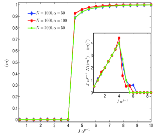
Figure 1: Magnetization (main figure) and its normalized fluctuations (inset) for systems of different sizes and different dilution as a function of $J\;\alpha^{p-1}$. Left panel: $p=2$, right panel $p=3$. The collapse of all the curves provides a strong evidence for the scaling of the interaction strength, coupled to the connectivity.

In general, we find that the system is able to relax to a well-defined steady state characterized by average observables (such as total energy and magnetization) which are independent of the initial configuration and of the system size $N$, as long as $N$ is large enough to avoid finite-size effects. On the other hand, the average observables vary as the average coordination number $\alpha$ and/or the interaction strength $J$ are tuned. In particular, as shown in Fig. $1$ we find that the curves for the order parameter collapse when plotted as a function of $J\;\alpha^{p-1}$, confirming the scaling found analytically. We also notice that the system exhibits a phase transition at a critical interaction strength $J_{c}$, which depends on the connectivity of the underlying network according to $J_{c}=\alpha^{-1}$ for $p=2$ and $J_{c}=4\alpha^{-2}$ for $p=3$. The existence of a phase transition is also confirmed by the corresponding peak displayed by the fluctuations of the order parameter $\langle m^{2}\rangle-\langle m\rangle^{2}$, see insets in Fig. $1$.

Before concluding, we stress the non-trivial role played by the connectivity of the social network: while for pair-wise interactions ($p=2$) $\alpha$ weights linearly, when interactions involve contemporary a number of agents larger than two ($p>2$), its weight gets more and more important. As a result, when $p$ is large, a full consensus within the system, i.e. a ferromagnetic state, can be reached at relatively small critical strengths with respect to the $p=2$ case usually analyzed, or, otherwise stated, relatively small coupling strengths among agents are sufficient to orient most part on the social system ERP .

References

- (1) E. Agliari, A. Barra, F.Camboni, Criticality in diluted ferromagnet, J. Stat. Mech. , (2008).
- (2) E. Agliari, R. Burioni, P. Contucci, A diffusive strategy in group competition, submitted.
- (3) E. Agliari, A. Barra, R. Burioni, P. Contucci, Effective interaction in group competition diffusive dynamics with strategies, to appear.
- (4) A. Barra The mean field Ising model trought interpolating techniques, J. Stat. Phys. 132, , (2008).
- (5) A. Barra Notes on ferromagnetic P-spin and REM, Math. Meth. Appl. Sc. 10, , (2008).
- (6) A. Barra, F.Camboni, P.Contucci, Dilution Robustness for Mean Field Diluted Ferromagnets, J. Stat. Mech. , (2009).
- (7) C.Berge, Graphs and hypergraphs, North-Holland Mathematical Library (1973).
- (8) W. Brock, S. Durlauf, Discrete Choice with Social Interactions, Review of Economic Studies, 68, , (2001).
- (9) R. Cont, M. Lowe, Social distance, heterogeneity and social interaction, Centre des Mathematiques Appliquees, Ecole Polytechnique, 505, (2003).
- (10) P. Contucci, C. Giardina’, Mathematics and Social Sciences: A Statistical Mechanics Approach to Immigration, ERCIM News, 73, 34, (2008).
- (11) S. Galam, Heterogeneous beliefs, segregation, and extremism in the making of public opinions, Phys. Rev. E, 71 046123 (2005).
- (12) I. Gallo, A. Barra, P. Contucci, A minimal model for the imitative behaviour in social decision making: theory and comparison with real data, Math. Mod. and Meth. in Appl. Sc., Special Issue: Mathematics and Complexity in Human and Life Sciences, (2008).
- (13) S. Graffi, P. Contucci (Ed.s), How Can Mathematics Contribute to Social Sciences, Special Issue of Quality and Quantity, 41, , (2007).
- (14) G. Caldarelli, Scale free networks, Cambridge Univerisity Press, (2008).
- (15) M. E. J. Newman and G. T. Barkema , Monte Carlo methods in Statistical Physics, Oxford University Press, 2001.