Comments on
“Particle Markov chain Monte Carlo”
by C. Andrieu, A. Doucet, and R. Hollenstein

Abstract

This note merges three discussions written by all or some of the above authors about the Read Paper “Particle Markov chain Monte Carlo” by C. Andrieu, A. Doucet, and R. Hollenstein, presented on October 16 at the Royal Statistical Society and to be published in the Journal of the Royal Statistical Society Series B.

1 Introduction

We congratulate the three authors for opening such a new vista for running MCMC algorithms in state-space models. Being able to devise a correct Markovian scheme based on a particle approximation of the target distribution is a genuine “tour de force” that deserves an enthusiastic recognition! This is all the more impressive when considering that the ratio

$$\widehat{p}_{\theta}(x_{1:T}^{\star}|y_{1:T})/\widehat{p}_{\theta}(x_{1:T}(i-1)|y_{1:T})$$

is not unbiased and thus invalidate the usual importance sampling solutions, as demonstrated by Beaumont et al., (2009). Thus, the resolution of simulating by conditioning on the lineage truly is an awesome resolution of the problem!

2 Implementation and code

We implemented the PHM algorithm for the (notoriously challenging) stochastic volatility model

$$y_{t}|x_{t}\sim\mathcal{N}(0,e^{x_{t}}),\quad x_{t}=\mu+\rho(x_{t-1}-\mu)+\sigma\varepsilon_{t}\,,$$

based on several hundred simulated observations. With parameter moves

$$\mu^{*} \sim\mathcal{N}(\mu,20^{-2}),$$

$$\rho^{*} \sim\mathcal{N}(\rho,20^{-2}),$$

$$\log{\sigma^{*}} \sim\mathcal{N}(\log\sigma,20^{-2}),$$

and state-space moves derived from the AR(1) prior, we obtained good mixing properties with no calibration effort, using $N=10^{2}$ particles and $10^{4}$ Metropolis–Hastings iterations, as demonstrated by Figures 1 and 2.

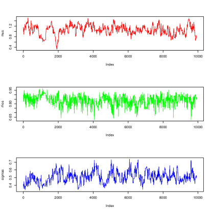
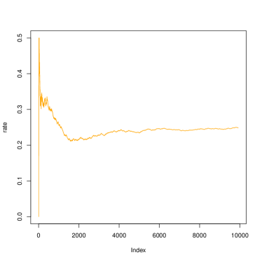
Figure 1: Evolution of the (left) parameter simulations for $\mu$, $\rho$ and $\sigma$, plotted against iteration indices and of the (right) estimated acceptance rate of the PMCMC algorithm, obtained $N=10^{2}$ particles and $10^{4}$ Metropolis–Hastings iterations and a simulated sequence of $500$ observations with true values $\mu_{0}=1$, $\rho_{0}=0.9$ and $\sigma_{0}=0.5$.

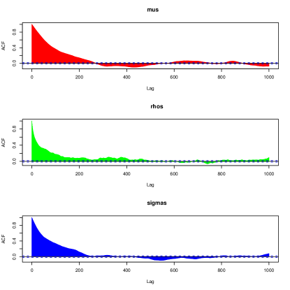
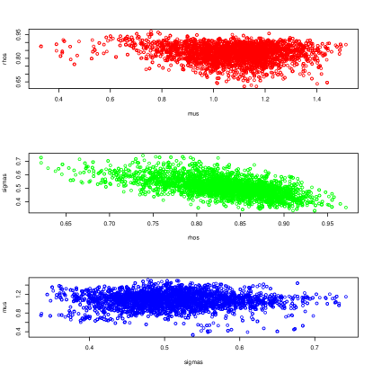
Figure 2: Autocorrelation (left) and pairwise (right) graphs for the $\mu$, $\rho$ and $\sigma$ sequences for the same target as in Figure 1.

The acceptance rate for this configuration, when using a variance of $0.05^{2}$ for each parameter move, and $100$ particles for $500$ observations, was around 25%. With $100$ observations and $100$ particles, the results of the PHM algorithm showed a bimodality in the Markov chain as presented in Figure 3.

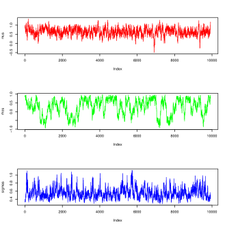
(a) Parameter values.

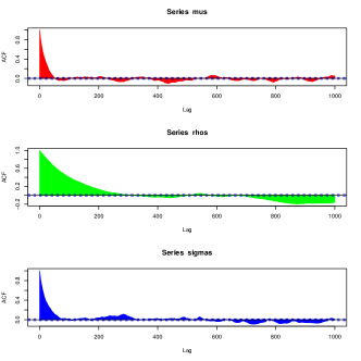
(b) Autocorrelograms.

Figure 3: Evolution of the (left) parameter simulations for $\mu$, $\rho$ and $\sigma$, plotted against iteration indices, and autocorrelograms for $\mu$, $\rho$ and $\sigma$, for $100$ observations and $100$ particles.

The sequence of the $\rho$’s on the lhs of Figure 3 exhibits concentrations around both $0.9$ and $-0.9$. This bimodality of the posterior on $\rho$ disappears when the number of observations grows, as shown by Figures 2 and 4, obtained with $1000$ simulated observations and $1000$ particles.

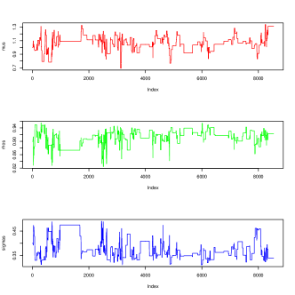
(a) Parameter values.

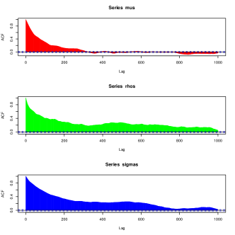
(b) Autocorrelograms.

Figure 4: Evolution of the (left) parameter simulations for $\mu$, $\rho$ and $\sigma$, and autocorrelograms for $\mu$, $\rho$ and $\sigma$, plotted against iteration indices, for $1000$ observations and $1000$ particles.

Bimodality of the posterior on $\rho$ could possibly occur for a larger number of observations. It may also be an artifact of the simulation method, which would require a higher number of particles or of iterations to assess. Unfortunately, this is computationally very demanding: using our Python programme on $10,000$ iterations, $1000$ observations and $1000$ particles requires five hours on a mainframe computer.

Figures 3 and 4, obtained with the same proposal variance, also illustrate the severe decrease in the acceptance rate when the number of observations grows: the proposed parameter values get rejected for more than 100 iterations in a row on Figure 4.

Our computer program is written in the Python language. It is available for download at http://code.google.com/p/py-pmmh/ and may be adapted to any state-space model by simply rewriting two lines of the code, namely those that (a) compute $p(y_{t}|x_{t})$ and (b) simulate $x_{t+1}|x_{t}$. Contemplating a different model does not even require the calculation of full conditionals, in contrast to Gibbs sampling. Another advantage of the py-pmmh algorithm is that it is trivial to parallelise. (Adding a comment before the loop over the particle index is enough, using the OpenMP technology.)

3 Recycling

Although this is already addressed in the last section of the paper, we mention here possible options for a better recycling of the numerous simulations produced by the algorithm. This dimension of the algorithm deserves deeper study, maybe to the extent of allowing for a finite time horizon overcoming the MCMC nature of the algorithm, as in the PMC solution of Cappé et al., (2008).

A more straightforward remark is that, due to the additional noise brought by the resampling mechanism, more stable recycling would be produced both in the individual weights $\omega_{n}(X_{1:n})$ by Rao–Blackwellisation of the denominator in eqn. (7) as in Iacobucci et al., (2009) and over past iterations by a complete reweighting scheme like AMIS (Cornuet et al.,, 2009). Another obvious question is whether or not the exploitation of the wealth of information provided by the population simulations is manageable via adaptive MCMC methods (Andrieu and Robert,, 2001; Roberts and Rosenthal,, 2009)

4 Model choice

Since

$$\widehat{p}_{\theta}(y_{1:T})=\widehat{p}_{\theta}(y_{1})\prod_{n=2}^{T}\widehat{p}_{\theta}(y_{n}|y_{1:n-1})$$

is an unbiased estimator of $p_{\theta}(y_{1:T})$, there must be direct implications of the method towards deriving better model choice strategies in state-space models, as exemplified in Population Monte Carlo by Kilbinger et al., (2009) in a cosmology setting.

In fact, the paper does not cover the corresponding calculation of the marginal likelihood $p(y)$, the central quantity in model choice. However, the PMCMC approach seems to lend itself naturally to the use of Chib’s (1995) estimate, i.e.

$$p(y)=\frac{p(\theta^{\star})p(y|\theta^{\star})}{p(\theta^{\star}|y)}$$

for any $\theta^{\star}$. Provided the $p(\theta|x,y)$ density allows for a closed-form expression, the denominator may be estimated by

$$p(\theta|y)=\int p(\theta|x,y)p(x|y)\,\text{d}x\approx\frac{1}{M}\sum_{i=1}^{M}p(\theta|x=x_{i},y)\,,$$

where the $x_{i}$’s, $i=1,...,M,$ are provided by the MCMC output.

The novelty in Andrieu et al. (2009) is that $p(y|\theta)$ in the numerator needs to be evaluated as well. Fortunately, as pointed out above, each iteration $i$ of the PMCMC sampler provides a Monte Carlo estimate of $p(y|\theta=\theta_{i})$, where $\theta_{i}$ is the current parameter value. Some care may be required when choosing $\theta^{\star}$; e.g. selecting the $\theta^{\star}$ with largest (evaluated) likelihood may lead to a biased estimator.

We did some experiments in order to compare the approach described above with INLA (Rue et al.,, 2009) and nested sampling (Skilling,, 2007; see also Chopin and Robert,, 2007), using the stochastic volatility example of Rue et al. (2009). Unfortunately, our PMCMC program requires more than one day to complete (for a number $N$ of particles and a number $M$ of iterations that are sufficient for reasonable performance), so we were unable to include the results in this discussion. A likely explanation is that the cost of PMCMC is at least $O(T^{2})$, where $T$ is the sample size ($T=945$ in this example), since, according to the authors, good performance requires than $N=O(T)$, but our implementation may be sub-optimal as well.

Interestingly, nested sampling performs reasonably well on this example (reasonable error obtained in one hour), and, as reported by Rue et al., (2009), the INLA approximation is fast (one second) and very accurate, but more work is required for a more meaningful comparison.

5 Connections with some of the earlier literature

Two interesting metrics for the impact of a Read Paper are: (a) the number of previous papers it impacts in some way; and (b) the number of interesting theoretical questions it opens. In both respects, this paper fares very well.

Regarding (a), in many complicated models the only tractable operations are state filtering and likelihood evaluation, as shown, e.g., in the continuous-time model of Chopin and Varini, (2007). In such settings, the PHM algorithm offers Bayesian estimates “for free”, which is very nice.

Similarly, Chopin, (2007), see also Fearnhead and Liu, (2007), formulates change-point models as state-space models, where the state $x_{t}=(\theta_{t},d_{t})$, comprises the current parameter $\theta_{t}$ and the time since the last change $d_{t}$. In this setting, one may use SMC to recover the trajectory $x_{1:T}$, i.e., all the change dates and parameter values. It works well when $x_{t}$ forgets about its past quickly enough, but this forbids hierarchical priors for the durations and the parameters. PHM removes this limitation: Chopin’s (2007) SMC algorithm may indeed be embedded into a PHM algorithm, where each iteration corresponds to a different value of the hyper-parameters. This comes as a cost however, as each MCMC iteration need run a complete SMC algorithm.

Regarding point (b), several questions, which have already been answered in the standard SMC case, may again be asked about PMCMC: Does residual resampling outperform multinomial resampling? Is the algorithm with $N+1$ particles strictly better than the one with $N$ particles? What about Rao-Blackwellisation, or the choice of the proposal distribution? One technical difficulty is that marginalising out components always reduces the variance in SMC, but not in MCMC. Another difficulty is that PMCMC retains only one particle trajectory $x_{1:T}$, hence the impact in reducing variability between particles is less immediate.

Similarly, obtaining a single trajectory $x_{1:T}$ from a forward filter is certainly much easier than obtaining many of them, but this may still be quite demanding in some scenarios, i.e., there may be so much degeneracy in $x_{1}$ that not a single particle does contain a $x_{1}$ that is in the support of $p(x_{1}|y_{1:T})$.

References

- Andrieu and Robert, (2001) Andrieu, C. and Robert, C. (2001). Controlled Markov chain Monte Carlo methods for optimal sampling. Technical Report 0125, Université Paris Dauphine.
- Beaumont et al., (2009) Beaumont, M., Cornuet, J.-M., Marin, J.-M., and Robert, C. (2009). Adaptive approximate Bayesian computation. Biometrika, 96(3).
- Cappé et al., (2008) Cappé, O., Douc, R., Guillin, A., Marin, J.-M., and Robert, C. (2008). Adaptive importance sampling in general mixture classes. Statist. Comput., 18:447–459.
- Chib, (1995) Chib, S. (1995). Marginal likelihood from the Gibbs output. J. American Statist. Assoc., 90:1313–1321.
- Chopin, (2007) Chopin, N. (2007). Inference and model choice for time-ordered hidden Markov models. J. Royal Statist. Society Series B, 69(2):269–284.
- Chopin and Robert, (2007) Chopin, N. and Robert, C. (2007). Contemplating evidence: properties, extensions of, and alternatives to nested sampling. Technical Report 2007-46, CEREMADE, Université Paris Dauphine. arXiv:0801.3887.
- Chopin and Varini, (2007) Chopin, N. and Varini, E. (2007). Particle filtering for continuous-time hidden Markov models. ESAIM: Proceedings, Conference on Sequential Monte Carlo Methods, 19:12–17.
- Cornuet et al., (2009) Cornuet, J.-M., Marin, J.-M., Mira, A., and Robert, C. (2009). Adaptive multiple importance sampling. Technical Report arXiv.org:0907.1254, CEREMADE, Université Paris Dauphine.
- Fearnhead and Liu, (2007) Fearnhead, P. and Liu, Z. (2007). Online inference for multiple changepoint problems. J. Royal Statist. Society Series B, 69(3):589–605.
- Iacobucci et al., (2009) Iacobucci, A., Marin, J.-M., and Robert, C. (2009). On variance stabilisation by double Rao-Blackwellisation. Comput. Stati. Data Analysis. (To appear.).
- Kilbinger et al., (2009) Kilbinger, M., Wraith, D., Robert, C., and Benabed, K. (2009). Model comparison in cosmology. Technical report, Institut d’Astrophysique de Paris.
- Roberts and Rosenthal, (2009) Roberts, G. and Rosenthal, J. (2009). Examples of adaptive MCMC. J. Comp. Graph. Stat., 18:349–367.
- Rue et al., (2009) Rue, H., Martino, S., and Chopin, N. (2009). Approximate Bayesian inference for latent Gaussian models using integrated nested Laplace approximations. J. Royal Statist. Society Series B, 71:319–392.
- Skilling, (2007) Skilling, J. (2007). Nested sampling for general Bayesian computation. In Bernardo, J., Bayarri, M., Berger, J., David, A., Heckerman, D., Smith, A., and West, M., editors, Bayesian Statistics 8.