The Cross Section of the Process $e^{+}+e^{-}\rightarrow J/\psi+\eta_{c}$ within the QCD Light-Cone Sum Rules

Abstract

We calculate the cross section of the exclusive process $e^{+}+e^{-}\rightarrow J/\psi+\eta_{c}$ at the leading order approximation within the QCD light-cone sum rules approach. It is found that the form factor $F_{VP}(V=J/\psi,P=\eta_{c})$ depends mainly on the behavior of the twist-2 distribution amplitude of the $\eta_{c}$-meson at the scale of this process. Thus in order to obtain a reliable estimation of the cross section, it is important to have a realistic distribution amplitude of the $\eta_{c}$ meson, and to deal with the evolution of the distribution amplitude to the effective energy scale of the process. Our results show that one can obtain a compatible prediction with the Belle and BaBar experimental data.

PACS numbers: 11.55.Hx, 12.38.Lg, 12.39.-x, 14.40.Lb

I introduction

The double-charmonium production in $e^{+}e^{-}$ annihilation at the B factory provides a good platform to study both perturbative and non-perturbative effects in quantum chromodynamics (QCD).

On one hand, from the experimental point of view, the cross section of the precess $e^{+}+e^{-}\rightarrow J/\psi+\eta_{c}$ was measured at Belle Belle2002 ; Belle2004 and BaBar BaBar2005 , and their recent observation show that Belle2002 ; BaBar2005

$$\sigma(e^{+}+e^{-}\rightarrow J/\psi+\eta_{c})\times{{\cal B}_{>2}}=25.6\pm 2.8\pm 3.4\;{\rm fb}\;\;({\rm Belle})$$

and

$$\sigma(e^{+}+e^{-}\rightarrow J/\psi+\eta_{c})\times{{\cal B}_{>2}}=17.6\pm 2.8^{+1.5}_{-2.1}\;{\rm fb}\;\;({\rm BaBar}),$$

where ${{\cal B}_{>2}}$ denotes the branching fraction for the final states with more than two charged tracks.

On the other hand, from the theoretical point of view, the process $e^{+}+e^{-}\rightarrow J/\psi+\eta_{c}$ is usually studied within the nonrelativistic QCD (NRQCD) BBL1997 . Under the leading order (LO) NRQCD calculation, Refs.BLB2003 ; BL2003 ; Chao2003 derived a much smaller cross section $\sigma=3.78\sim 5.5\;{\rm fb}$ for the first time. Thus there are large discrepancy between theoretical predictions of the LO NRQCD calculation and the experimental measurements. In order to solve this problem, many attempts were made based on the NRQCD approach. Refs.Chao2006 ; Wang2008 diminished the disagreement to a large degree by including the radiative correction. Moreover, as pointed out in Refs.BKKY2007 ; Chao2007 ; BLC2008 , the relativistic corrections can further improve the accuracy. By taking both the radiative and relativistic corrections into account, Ref.BLC2008 got $17.6^{+8.1}_{-6.7}\;{\rm fb}$, then the authors there optimistically concluded that the disagreement between theoretical predictions in NRQCD approach and experiments has been resolved BLC2008 . However, one may doubt the validity of the $\alpha_{s}$- and $v^{2}$- expansion in the process $e^{+}+e^{-}\rightarrow J/\psi+\eta_{c}$, if the LO result is an order of magnitude smaller than the experimental measurements and the next-to-leading order (NLO) corrections/higher $v^{2}$-expansion terms inversely play a dominate role for the double charmonium production. Furthermore, Ref.Wang2008 showed that the scale dependence of the cross section can not be improved even with the NLO correction, so it is an important matter to determine the typical scale of the process or at least to make a more reliable estimation of scale dependence.

In contrast, it was argued that the experimental results by Belle and BaBar collaborations of the process $e^{+}+e^{-}\rightarrow J/\psi+\eta_{c}$ can also be explained by using the perturbative QCD (pQCD) with proper models for the charmonium distribution amplitudes (DA) BC2005 . They claimed, “the difficulties in explaining the Belle and BaBar results for $\sigma(e^{+}+e^{-}\rightarrow J/\psi+\eta_{c})$ are not really the difficulties of QCD, but are rather due to a poor approximation of the real dynamics of $c$-quarks by NRQCD”. Actually, the exclusive process can be factorized into two parts in the pQCD approach: the calculable hard-parton amplitude and the hadronic distribution amplitude. If one replaces all DAs in the pQCD formulae by a simple $\delta$ function, the calculated cross section will be back to a few $fb$ that is consistent with the NRQCD approach. However one always assume that the hadronic distribution amplitude is not non-relativistic. Therefore, the key point is that the relativistic DA, instead of the $\delta$ function, enhances the cross section of the process $e^{+}+e^{-}\rightarrow J/\psi+\eta_{c}$.

Furthermore, since the QCD light-cone sum rules (LCSR) combines the QCD sum rules and the pQCD theory of hard exclusive processes in a suitable way, it can be a good tool for calculating the form factors in the large momentum transfer. For example, LCSR is a successful method for dealing with the $\gamma^{*}\rho\rightarrow\pi$ transition form factor K1999 that is similar to the process $e^{+}+e^{-}\rightarrow J/\psi+\eta_{c}$. We shall try to apply the QCD LCSR approach to calculate the amplitude of the process $e^{+}+e^{-}\rightarrow V+P$, where $V=J/\psi,...$ and $P=\eta_{c},...$. The theoretical predictions at the LO approximation for the cross section of the process $e^{+}+e^{-}\rightarrow V+P$ at the large energy scale can be obtained by using the QCD LCSR. Similar to the pQCD approach, this method also faces two problems: which charmonium DA model should be adopted and how large effects can be determined by the DA evolution. In the present paper, we shall discuss the behavior of the different models for the charmonium DA and the effects of the renormalized group evolution with the effective scale in the process.

The remaining parts of the paper are organized as follows. In Sec. II, we present calculation technology for $e^{+}+e^{-}\rightarrow J/\psi+\eta_{c}$ under the QCD LCSR, where the leading-twist DA is constructed and its QCD evolution is presented. Numerical results for the cross section of the process $e^{+}+e^{-}\rightarrow J/\psi+\eta_{c}$ are presented in Sec. III. The final section is reserved for summary and conclusion.

II Calculation technology for $e^{+}+e^{-}\rightarrow J/\psi+\eta_{c}$

Generally, the cross section for the process $a(p_{1})+b(p_{2})\rightarrow c(p_{3})+d(p_{4})$ is given by

$$\sigma=\frac{1}{4E_{1}E_{2}v_{rel}}\int\frac{d^{3}\vec{p}_{3}d^{3}\vec{p}_{4}}{(2\pi)^{3}2E_{3}(2\pi)^{3}2E_{4}}(2\pi)^{4}\delta^{4}(p_{1}+p_{2}-p_{3}-p_{4})|\overline{\cal M}|^{2},$$ (1)

where $p_{i}=(E_{i},\vec{p}_{i})$ $(i=1,\cdots,4)$ stand for the four-momentum of initial and final particles correspondingly, $v_{rel}=|\frac{\vec{p_{1}}}{E_{1}}-\frac{\vec{p_{2}}}{E_{2}}|$. $|\overline{\cal M}|^{2}$ is the squared absolute value of the matrix element, where the color states and spin projections of the initial and final particles have been summed up and those of the initial particles have been averaged.

For the exclusive double-charmonium production $e^{+}+e^{-}\rightarrow J/\psi+\eta_{c}$, its Lorentz-invariant matrix element turns out to be

$${\cal M}=i\int d^{4}x{<}J/\psi\eta_{c}|T\left\{Q_{c}J^{c}_{\mu}(x)A^{\mu}(x),\bar{e}(0)\gamma_{\nu}e(0)A^{\nu}(0)\right\}|e^{+}e^{-}>,$$ (2)

where $J^{c}_{\mu}(x)=\bar{C}(x)\gamma_{\mu}C(x)$ is the $c$-quark electromagnetic current. Then, we obtain

$$|\overline{\cal M}|^{2}=2Q_{c}^{2}|F_{VP}|^{2}\frac{(S-4m_{J/\psi}^{2})}{4S}\left[1+\cos^{2}\theta\right],$$ (3)

where $\theta$ is the scattering angle, $Q_{c}=\frac{2}{3}$ is the charm quark charge and the form factor $F_{VP}$ is defined as

$${<}J/\psi(P-q)\eta_{c}(P)|J^{c}_{\mu}(0)|0{>}=\epsilon_{\mu abc}\epsilon^{a*}q^{b}P^{c}F_{VP},$$ (4)

with $\epsilon^{a}$ being the polarization vector of $J/\psi$-meson and $S=-q^{2}$. Neglecting the small mass difference between $J/\psi$ and $\eta_{c}$ mesons, the cross section becomes

$$\sigma = \frac{\pi\alpha^{2}Q_{c}^{2}}{6}\left(1-\frac{4m_{J/\psi}^{2}}{S}\right)^{3/2}|F_{VP}|^{2}.$$ (5)

It is shown that the main part is to calculate the form factor $F_{VP}$. There are many methods to calculate it, such as NRQCD BLB2003 ; BL2003 ; Chao2003 ; Wang2008 ; Chao2006 ; BKKY2007 ; Chao2007 ; BLC2008 , PQCD BC2005 and light-cone perturbative QCD approaches CJ2007 ; Braguta2008 . Here we use the LCSR approach BBK1989 ; BF1989 ; CZ1990 ; CK2001 to calculate $F_{VP}$.

II.1 the form factor $F_{VP}$ within the QCD LCSR

We adopt the following two-point correlator to calculate the form factor $F_{VP}$

$$\Pi_{\mu\nu}(P,q) = i\int d^{4}xe^{-iqx}{<}\eta_{c}(P)|T\{J^{c}_{\mu}(x)J^{c}_{\nu}(0)\}|0{>},$$ (6)

where $q$ is the four-momentum of the virtual photon, $P$ is the four-momentum of $\eta_{c}$ meson.

On one hand, by inserting a complete set of intermediate hadronic states in Eq.(6), we get

$$\Pi_{\mu\nu}(P,q)=-\epsilon_{\mu\nu\alpha\beta}q^{\alpha}P^{\beta}F_{VP}f_{J/\psi}\frac{1}{m_{J/\psi}^{2}-(q-P)^{2}}+\frac{1}{\pi}\int_{s_{0}}^{\infty}ds\frac{{\rm Im}F_{\mu\nu}}{s-(q-P)^{2}},$$ (7)

where the decay constant $f_{J/\psi}$ is defined as, ${<}0|J^{c}_{\mu}(0)|J/\psi(P-q){>}=f_{J/\psi}m_{J/\psi}\epsilon_{\mu}$, with $\epsilon^{\mu}$ being the polarization vector of $J/\psi$-meson. $s_{0}$ is the threshold parameter whose value can be taken as $3.6^{2}~{}\mbox{GeV}^{2}<s_{0}<4.2^{2}~{}\mbox{GeV}^{2}$ EJ2001 . The second term in Eq.(7) is the dispersion integral that includes the contributions from the excited and continuum states in the region $s>s_{0}$.

On the other hand, the correlation function Eq.(6) can also be calculated by expanding the $T$-product of quark currents near the light cone $x^{2}=0$ due to sufficiently large momentum transfer. For such purpose, we contract the two $c$-quark fields and write down a free $c$-quark propagator

$$\overline{C(x)\bar{C}(0)} = iS(x,0)=i\int\frac{d^{4}k}{(2\pi)^{4}}e^{-ikx}\frac{\not\!k+m_{c}}{k^{2}-m_{c}^{2}}.$$ (8)

Then up to twist-3 accuracy, Eq.(6) can be simplified as

$$\Pi_{\mu\nu}^{QCD}(P,q) = 2\epsilon_{\mu\rho\nu\tau}q^{\rho}P^{\tau}f_{\eta_{c}}\int_{0}^{1}dx\frac{\phi_{\eta_{c}}(x)}{m_{c}^{2}-(xP-q)^{2}},$$ (9)

where $m_{c}$ is the current $c$-quark mass, $f_{\eta_{c}}$ is the decay constant of ${\eta_{c}}$ meson, $\phi_{\eta_{c}}$ stands for the $\eta_{c}$ leading-twist DA that is defined through the matrix element:

$${<}\eta_{c}(P)|\bar{C}(x)\gamma^{\tau}\gamma_{5}C(0)|0{>} = -iP^{\tau}f_{\eta_{c}}\int_{0}^{1}due^{iuPx}\phi_{\eta_{c}}(u)+{\rm higher\;twist\;terms}.$$ (10)

Next, by applying the quark-hadron duality to Eq.(7) and by applying the Borel transformation SVZ1979

$${\cal B}_{M^{2}}\frac{1}{m^{2}_{J/\psi}-(q-P)^{2}} = \frac{1}{M^{2}}e^{-\frac{m^{2}_{J/\psi}}{M^{2}}},$$

$${\cal B}_{M^{2}}\frac{1}{m^{2}_{c}-(q-xP)^{2}}, = \frac{1}{xM^{2}}e^{\left\{-\frac{1}{xM^{2}}\left[m^{2}_{c}+x(1-x)P^{2}-(1-x)q^{2}\right]\right\}},$$ (11)

to Eq.(7) and Eq.(9), we obtain the sum rule for $F_{VP}$

$$F_{VP} = \frac{2f_{\eta_{c}}}{m_{J/\psi}f_{J/\psi}}\int_{\Delta}^{1}dx\frac{\phi_{\eta_{c}}(x)}{x}e^{\left\{-\frac{1}{xM^{2}}\left[m_{c}^{2}+x(1-x)m_{\eta_{c}}^{2}+(1-x)Q^{2}\right]+\frac{m_{J/\psi}^{2}}{M^{2}}\right\}},$$ (12)

where $\Delta=\frac{1}{2m_{\eta_{c}}^{2}}\left[\sqrt{(s_{0}-m_{\eta_{c}}^{2}+Q^{2})^{2}+4(m_{c}^{2}+Q^{2})m_{\eta_{c}}^{2}}-(s_{0}-m_{\eta_{c}}^{2}-q^{2})\right]$, $M^{2}$ is the Borel transformation parameter and $P^{2}=m_{\eta_{c}}^{2}$, $-q^{2}=Q^{2}=S=112\mbox{GeV}^{2}$. It is found that the form factor $F_{VP}$ depends heavily on the DA $\phi_{\eta_{c}}$, especially on its end point behavior due to $\Delta\sim 0.9$.

II.2 leading-twist DA of $\eta_{c}$ meson

The key input for the form factor is the gauge-independent and process-independent DA $\phi_{\eta_{c}}$, which is of non-perturbative nature and can be defined as the integral of the valence Fock wave function LB1980

$$\phi_{\eta_{c}}(x,\mu_{0}) = \frac{2\sqrt{6}}{f_{\eta_{c}}}\int_{|\vec{k_{\perp}}|^{2}<\mu_{0}^{2}}\frac{d^{2}\vec{k_{\perp}}}{16\pi^{3}}\Psi_{\eta_{c}}(x,\vec{k}_{\perp}),$$ (13)

where $\mu_{0}$ stands for the separation scale between the perturbative and non-perturbative regions. As for a scale $\mu>\mu_{0}$, the non-perturbative DA $\phi_{\eta_{c}}(x,\mu)$ is given by the renormalization group evolution that can be calculated perturbatively.

Table 1: The explicit form of the spin-space wave function $\chi^{\lambda_{1}\lambda_{2}}(x,\vec{k}_{\perp})$, where the transverse momentum $\vec{k}_{\perp}=(k_{x},k_{y})$ and $m_{c}^{*}$ stands for the constituent $c$-quark mass.

$\lambda_{1}\lambda_{2}$	$\uparrow\uparrow$	$\uparrow\downarrow$	$\downarrow\uparrow$	$\downarrow\downarrow$
$\chi^{\lambda_{1}\lambda_{2}}(x,\vec{k}_{\perp})$	$-\frac{k_{x}-ik_{y}}{\sqrt{2(m^{*2}_{c}+k_{\perp}^{2})}}$	$\frac{m^{*}_{c}}{\sqrt{2(m^{*2}_{c}+k_{\perp}^{2})}}$	$-\frac{m^{*}_{c}}{\sqrt{2(m^{*2}_{c}+k_{\perp}^{2})}}$	$-\frac{k_{x}+ik_{y}}{\sqrt{2(m^{*2}_{c}+k_{\perp}^{2})}}$

Up to now, it is difficult to give the light-cone wave function (LCWF) from the first principles of QCD. So one usually constructs some phenomenological models for the wave function, such as BC model BC2005 , BKL model BKL2006 , BLL model BLL2007 , MS model MS2004 , BHL model BHL1981 and etc. Here, we shall take the BHL model for the $\eta_{c}$ wave function, which can be written as HZ2007

$$\Psi^{\lambda_{1}\lambda_{2}}_{\eta_{c}}(x,\vec{k}_{\perp})=\varphi_{\mathrm{BHL}}(x,\vec{k}_{\perp})\chi^{\lambda_{1}\lambda_{2}}(x,\vec{k}_{\perp})=Ae^{-b^{2}\frac{\vec{k_{\perp}}^{2}+m_{c}^{*2}}{x(1-x)}}\chi^{\lambda_{1}\lambda_{2}}(x,\vec{k}_{\perp}),$$ (14)

where $m_{c}^{*}$ stands for the constituent $c$-quark mass, $\lambda_{1}$ and $\lambda_{2}$ are helicity states of the constitute $c$ and $\bar{c}$ quarks, $\chi^{\lambda_{1}\lambda_{2}}(x,\vec{k}_{\perp})$ stands for the spin-space wave function coming from the Wigner-Melosh rotation M1974 . $\chi^{\lambda_{1}\lambda_{2}}(x,\vec{k}_{\perp})$ can be found in Refs.spin1 ; spin2 ; spin3 , whose explicit form is shown in TAB.1.

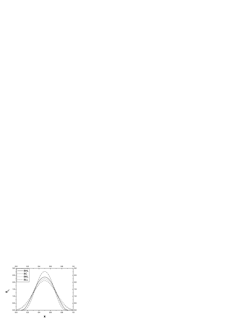
Figure 1: The comparison of the $\eta_{c}$ DAs of BHL model with those of BC BC2005 , BKL BKL2006 , BLL BLL2007 and BHL models at the initial scale $\mu_{0}$.

The parameters $A$ and $b^{2}$ can be determined by two constraints. One constraint is from the wave function normalization

$$\frac{2\sqrt{6}}{f_{\eta_{c}}}\int_{0}^{1}dx\int_{|\vec{k_{\perp}}|^{2}<\mu_{0}^{2}}\frac{d^{2}\vec{k_{\perp}}}{16\pi^{3}}\sum_{\lambda_{1}\lambda_{2}}\Psi^{\lambda_{1}\lambda_{2}}_{\eta_{c}}(x_{i},\vec{k}_{\perp})=1.$$ (15)

It can be found that only the usual helicity components $\lambda_{1}+\lambda_{2}=0$ makes contribution to the wave function normalization. More explicitly, from TAB.1, we have $\chi^{\lambda_{1}+\lambda_{2}=0}(x,\vec{k}_{\perp})=\frac{Am_{c}^{*}}{\sqrt{k^{2}_{\perp}+m_{c}^{*2}}}$. Another constraint is from the probability of finding the leading Fock state $|c\bar{c}>$ in the $\eta_{c}$ Fock state expansion, i.e.

$$\int_{0}^{1}dx\int\frac{d^{2}\vec{k_{\perp}}}{16\pi^{3}}|\varphi_{\mathrm{BHL}}(x,\vec{k}_{\perp})|^{2}=P_{\eta_{c}},$$ (16)

with $P_{\eta_{c}}\simeq 0.8$ spin1 . One can assume $\mu_{0}=m_{c}^{*}$ to be the initial scale for the non-perturbative distribution amplitude of the $\eta_{c}$-meson. Inputting the constituent quark mass $m_{c}^{*}=1.8~{}\mbox{GeV}$ BC2005 , the decay constant $f_{\eta_{c}}=0.335~{}\mbox{GeV}$ Yao2006 and the initial scale $\mu_{0}=m_{c}^{*}=1.8~{}\mbox{GeV}$, we get the corresponding parameters for $A=285.64291~{}\mbox{GeV}^{-1},b^{2}=0.19057~{}\mbox{GeV}^{-2}$. We compare the $\eta_{c}$-DA of our BHL model at the scale $\mu_{0}$ with those of BC BC2005 , BKL BKL2006 , BLL BLL2007 models in Fig.(1).

However, the scale $\mu$ of the form factor (12) that is at the B-factory is very different from the initial scale $\mu_{0}$ of $\eta_{c}$ DA. When DA runs to a higher energy scale $\mu$, other than $\mu_{0}$, with a proper QCD evolution, the behavior of DA shall be changed to a certain degree, especially in its upper end-point regions $\Delta<x<1$ that determines the form factor $F_{VP}$ as shown by Eq.(12). Therefore, it is quite important to do the DA evolution from the initial scale $\mu_{0}$ to a typical energy scale $\mu$ of the process so as to derive a more reliable cross section for $e^{+}+e^{-}\to J/\psi+\eta_{c}$ process. Thus, the next section is devoted to deal with the evolution of the $\eta_{c}$ DA.

II.3 The evolution of the $\eta_{c}$ DA with the scale $\mu$

We describe the DA evolution according to Ref.LB1980 . In the light-cone gauge, the DA $\phi_{\eta_{c}}$ is related to the hadronic wave function $\Psi_{\eta_{c}}$, which is the Fourier transform of the positive-energy projection of the usual Bethe-Salpeter wave function evaluated at relative “light-cone time”, i.e.

$$\phi_{\eta_{c}}(x_{i},\mu) = \left(\ln\frac{\mu^{2}}{\Lambda^{2}}\right)^{-\gamma_{F}/\beta}\int_{|\vec{k_{\perp}}|^{2}<\mu^{2}}\frac{d^{2}\vec{k_{\perp}}}{16\pi^{3}}\Psi_{\eta_{c}}(x_{i},\vec{k}_{\perp}),$$ (17)

where the factor in front of the integral comes from the scale dependence due to vertex and self-energy insertions. An evolution equation is obtained by differentiating both sides of Eq.(17) with respect to $\mu^{2}$. To order ${\cal O}(\alpha_{s})$, we obtain an “evolution equation” LB1980

$$x_{1}x_{2}\mu^{2}\frac{\partial\,\tilde{\phi}_{\eta_{c}}(x_{i},\mu)}{\partial\,\mu^{2}}=C_{F}\frac{\alpha_{s}(\mu^{2})}{4\pi}\left\{\int_{0}^{1}[d\,y]V(x_{i},y_{i})\tilde{\phi}_{\eta_{c}}(y_{i},\mu)-x_{1}x_{2}\tilde{\phi}_{\eta_{c}}(x_{i},\mu)\right\},$$ (18)

where

$$V(x_{i},y_{i}) = 2C_{F}\left[x_{1}y_{2}\theta(y_{1}-x_{1})\left(\delta_{h_{1}\bar{h_{2}}}+\frac{\Delta}{(y_{1}-x_{1})}\right)+(1\leftrightarrow 2)\right],$$ (19)

$$\,[d\,y] = d\,y_{1}d\,y_{2}\delta(1-y_{1}-y_{2}),$$

$$\phi_{\eta_{c}}(x_{i},\mu) = x_{1}x_{2}\tilde{\phi}_{\eta_{c}}(x_{i},\mu),$$

$C_{F}=4/3$, $\delta_{h_{1}\bar{h_{2}}}=1$ when the $c$ and $\bar{c}$ helicities are opposite, and $\Delta\tilde{\phi}_{\eta_{c}}(y_{i},\mu)=\tilde{\phi}_{\eta_{c}}(y_{i},\mu)-\tilde{\phi}_{\eta_{c}}(x_{i},\mu)$. The running coupling constant $\alpha_{s}(\mu^{2})$ at the LO is given by $\alpha_{s}(\mu^{2})=\frac{4\pi}{b_{0}\ln\left(\frac{\mu^{2}}{\Lambda^{2}}\right)}$ with $b_{0}=25/3$. One explicit solution of Eq.(18) can be written in the following Gegenbauer expansion

$$\phi_{\eta_{c}}(x_{i},\mu) = x_{1}x_{2}\sum_{n=0}^{\infty}a_{n}\left(\ln\frac{\mu^{2}}{\Lambda^{2}}\right)^{-\gamma_{n}}C^{3/2}_{n}(x_{1}-x_{2}),$$ (20)

where the Gegenbauer polynomials $C^{3/2}_{n}$ are eigenfunctions of $V(x_{i},y_{i})$ and the corresponding eigenvalues are the “non-singlet” anomalous dimensions

$$\gamma_{n} = \frac{C_{F}}{\beta}\left(1+4\sum_{k=2}^{n+1}\frac{1}{k}-\frac{2\delta_{h_{1}\bar{h_{2}}}}{(n+1)(n+2)}\right)\geq 0.$$ (21)

The coefficients $a_{n}$ which are non-perturbative can be determined from the initial condition $\phi_{\eta_{c}}(x_{i},\mu_{0})$ by using the orthogonality relations for the Gegenbauer polynomials $C^{3/2}_{n}$.

Figure 2: $\eta_{c}$-DA derived with strict evolution (18) at some typical energy scales, where the left is for BHL model BHL1981 and the right is for BLL model BLL2007 . The solid lines, dashed lines and the dotted lines represent DA at $\mu=\mu_{0}$, $\mu=3.46~{}\mbox{GeV}$ and $\mu=5.00~{}\mbox{GeV}$ respectively.

Usually, one truncates the Gegenbauer expansion (20) with the first $3$ or $4$ terms ($n=0,2,4,6$ in our case) to obtain the behavior of DA at the higher energy scales. In this paper we solve the evolution equation Eq.(18) strictly to get the DA’s behavior at the large scale since DA’s behavior is very important for calculating the form factor of the process $e^{+}+e^{-}\rightarrow J/\psi+\eta_{c}$. The Eq.(18) and Eq.(20) are equivalent to each other if the Gegenbauer expansion converges quickly. The evolution of DA with the strict evolution (18) are shown in Fig.(2), where the solid lines represent the DAs at the initial energy scale $\mu_{0}=1.80~{}\mbox{G}eV$, the dashed lines and dotted lines represent the DAs at the energy scale $\mu=3.46~{}\mbox{G}eV$ and $\mu=5~{}\mbox{G}eV$ that are taken by Ref.BC2005 and Ref.BLL2007 respectively. It is shown that when the energy scale becomes larger, the DA becomes lower in the middle while becomes higher near the end point, till at last when the energy scale tends to infinity, the DA tends to a asymptotic form $\phi_{as}(x)=6x(1-x)$.

III numerical results and discussion

To calculate the form factor and the cross section of $e^{+}+e^{-}\rightarrow J/\psi+\eta_{c}$, we take $f_{J/\psi}=0.416~{}\mbox{GeV}$, $f_{\eta_{c}}=0.335~{}\mbox{GeV}$, $m_{J/\psi}=3.096916~{}\mbox{GeV}$ and $m_{\eta_{c}}=2.9798~{}\mbox{GeV}$ Ed2001 ; Am2008 . And to compare with the results in literature BC2005 , we take the $c$-quark current mass to be $m_{c}=1.2~{}\mbox{GeV}$. The Borel parameter $M^{2}$ ranges from 8 to 15 $\mbox{GeV}^{2}$, when at this range, both the form factor and the cross section are stable. As for the effective scale $\mu$ of the process $e^{+}+e^{-}\rightarrow J/\psi+\eta_{c}$, Ref.BC2005 suggested $\mu\approx\sqrt{k^{2}}\approx 3.46~{}\mbox{GeV}$ from the mean value of $<Z^{k}_{m}>\approx 0.80$ or from the coupling constant $<\alpha_{s}(k^{2})>\approx 0.263$. Another usually adopted scale is $\mu\approx\sqrt{S}/2\simeq 5~{}\mbox{GeV}$ BLL2007 . Here, we will take $\mu=3.46~{}\mbox{GeV}$ and $\mu=5.00~{}\mbox{GeV}$ to do our discussion.

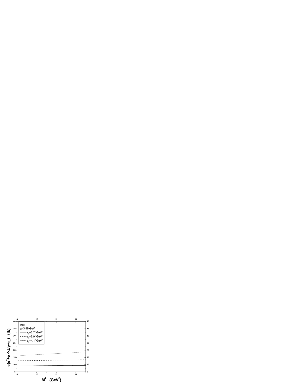
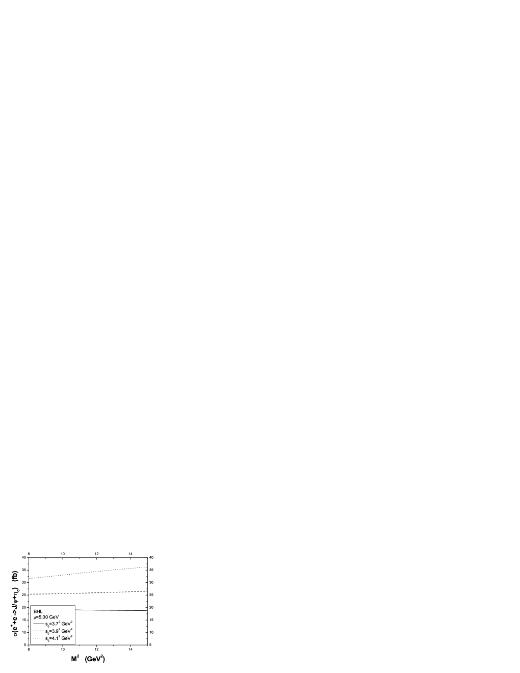
Figure 3: The dependance of cross section on the threshold parameter $s_{0}$ within the LCSR approach. The left and the right correspond to the scale $\mu=3.46~{}\mbox{GeV}$ and $\mu=5.00~{}\mbox{GeV}$ with the BHL model of $\eta_{c}$ DA.

As for the threshold parameter $s_{0}$, Ref.EJ2001 took $3.6^{2}~{}\mbox{GeV}^{2}<s_{0}<4.2^{2}~{}\mbox{GeV}^{2}$ EJ2001 with the central value $s_{0}=3.8^{2}~{}\mbox{GeV}^{2}$ as their case. Similarly, we also take $s_{0}$ within the same region while with a little different central value. To see the dependence of the cross section on the threshold parameter $s_{0}$, we give the cross section corresponding to $s_{0}=3.7^{2},\;\ 3.9^{2},\;\ 4.1^{2}~{}\mbox{G}eV^{2}$ with the BHL model at the scale $\mu=3.46~{}\mbox{GeV}$ and $\mu=5.00~{}\mbox{GeV}$ in Fig.(3). Since the cross section with the threshold parameter $s_{0}=3.9^{2}~{}\mbox{GeV}^{2}$ is more stable than that with $s_{0}=3.7^{2}~{}\mbox{GeV}^{2},\;\ 4.1^{2}~{}\mbox{GeV}^{2}$, we take $s_{0}=3.9^{2}~{}\mbox{GeV}^{2}$ as our central value of threshold parameter.

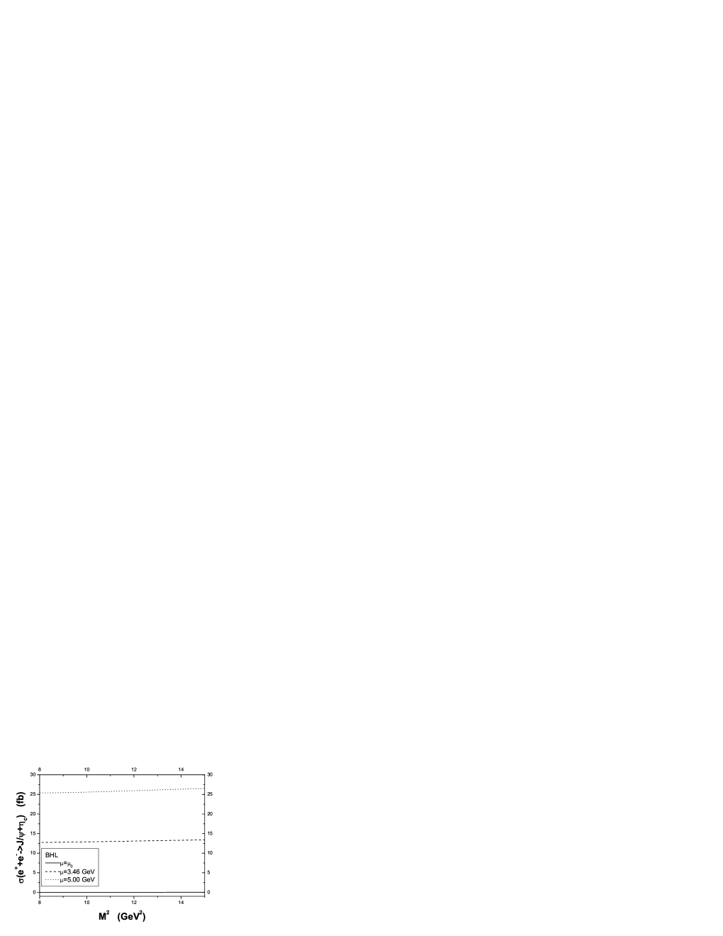
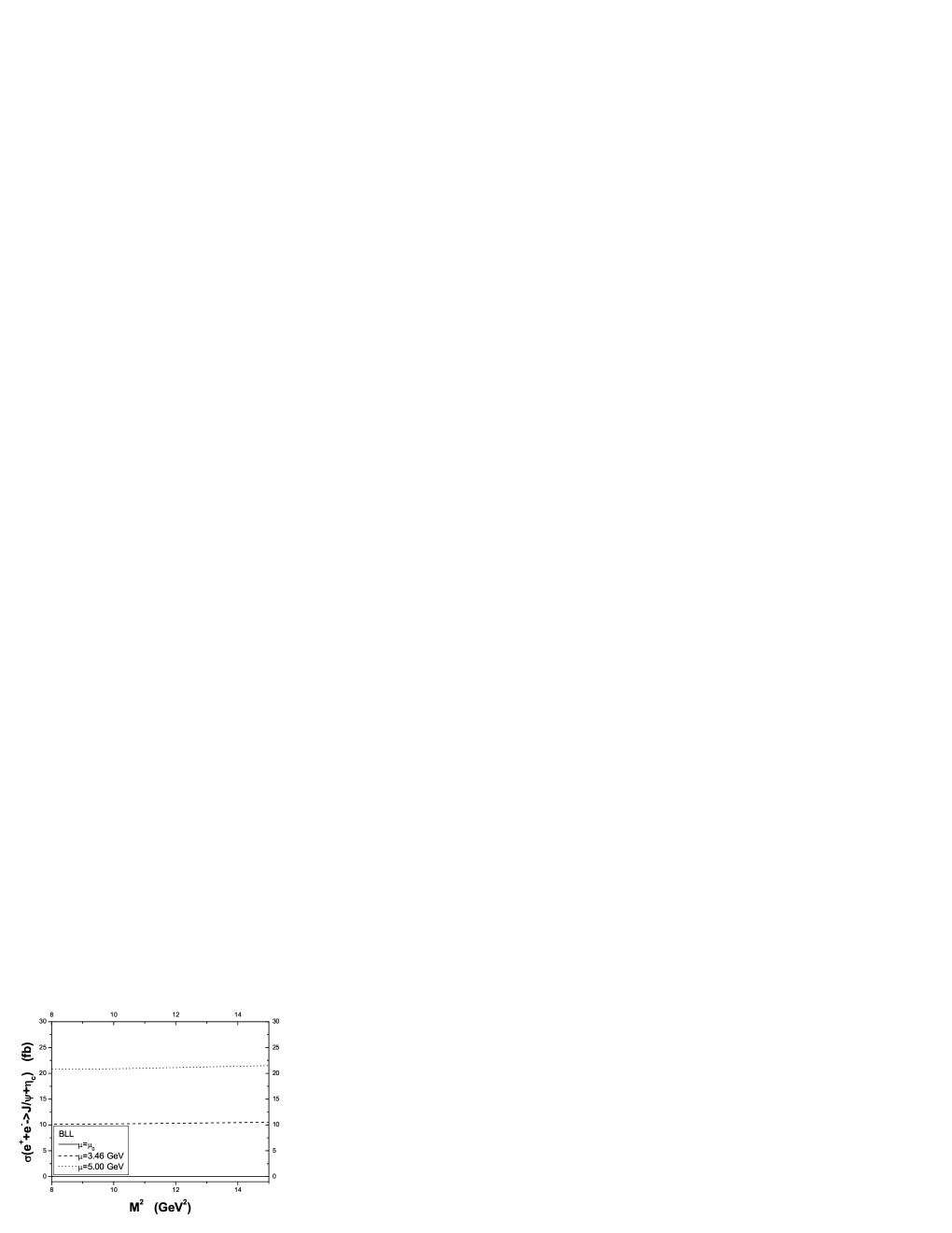
Figure 4: The cross section of $e^{+}+e^{-}\rightarrow J/\psi+\eta_{c}$ at different effective scale within the LCSR approach. The solid lines, dashed lines and dotted lines correspond to the $\eta_{c}$ meson distribution amplitude at the scale $\mu=\mu_{0}$, $\mu=3.46~{}\mbox{GeV}$ and $\mu=5.00~{}\mbox{GeV}$, where the left is for BHL model BHL1981 and the right is for BLL model BLL2007 .

Table 2: Comparison of the cross section of $e^{+}+e^{-}\rightarrow J/\psi+\eta_{c}$ from different $\eta_{c}$ DA models within the QCD light-cone sum rules approach.

$\phi$	BHL	BHL	BLL	BLL
$\mu~{}\mbox{(GeV)}$	3.46	5.00	3.46	5.00
$\sigma~{}\mbox{(\rm fb)}$	13.08$\pm$ 0.32	25.96$\pm$0.55	10.34$\pm$0.17	21.16$\pm$0.34

It is found that the cross section depends on the DA in the region $x>\Delta$ through the form factor formula (12). We show the cross section corresponding to three typical scales $\mu=\mu_{0}=1.80~{}\mbox{GeV}$, $\mu=3.46~{}\mbox{GeV}$ and $\mu=5.00~{}\mbox{GeV}$ in Fig.(4). When the effective energy scale increases, the corresponding cross section becomes bigger and is compatible with the BaBar and Belle’s measurements. Thus, by setting the effective energy scale and dealing with the DA evolution properly, the LCSR can provide a possible explanation for the double-charmonium production process $e^{+}+e^{-}\rightarrow J/\psi+\eta_{c}$ at the B factory. To explicate the cross sections of different models numerically, we further show these cross sections in Tab. 2, where the error is caused by the variation of $M^{2}$. One may observe that the cross section by BLL model is smaller than that by BHL model since the DA of the BLL model is narrower than that of the BHL model as shown in Fig.(2).

The above calculation is done at the LO approximation within the QCD LCSR and the error is only caused by the variation of the Borel parameter $M^{2}$. Of course, one should include the higher order contributions, such as the NLO corrections to the light-cone sum rules, the higher-twist DAs, the higher Fock states and etc. Therefore we can not estimate all of the uncertainties of the calculated cross section before doing a further study.

IV summary

The exclusive charmonium $J/\psi+\eta_{c}$ production in $e^{+}e^{-}$ collision is a very interesting problem. Since the discrepancy between theoretical prediction of the LO NRQCD and experimental data given by Belle and BaBar at the B factory has posed a significant challenge for several years, many theoretical attempts have been made to solve this challenging problem. It is worthwhile to study this process by taking various applicable approaches to understand the charmonium production dynamics. In this paper we study this process by using the QCD LCSR approach.

Our results based on the LCSR approach shows that the cross section of the process $e^{+}+e^{-}\rightarrow J/\psi+\eta_{c}$ substantially depends on the behavior of the $\eta_{c}$ DA at the energy scale $\mu$. Noticing that the energy scale $\mu$ at the B factory is greater than the initial scale $\mu_{0}$ of the $\eta_{c}$ DA, the renormalization group evolution of the DA has to be taken into account. The perturbative radiative correction leads to a big change of the DA especially to the tail of the DA at the large scale $\mu$.

At the present, one has poor knowledge of the DA and tries to build various models that have quite different behavior, especially at the end-point region. We stress that the evolution of the $\eta_{c}$ DA can give more reasonable prediction to the process $e^{+}+e^{-}\rightarrow J/\psi+\eta_{c}$ within the LCSR approach. Similar to other approaches, in order to calculate the cross section of the double-charmonium production one needs to have more knowledge of the charmonium DA.

The numerical results show that the cross section of the process $e^{+}+e^{-}\rightarrow J/\psi+\eta_{c}$ is predicted in the range $13\sim 26fb$. The calculated values for the different models can be compatible with the Belle and BaBar measurements by properly choosing effective energy scale for this process and dealing with the DA evolution effect.

Acknowledgments: This work was supported in part by Natural Science Foundation of China under Grant No.10675132, No.10735080 and No.10805082, and by Natural Science Foundation Project of CQ CSTC under Grant No.2008BB0298.

References

- (1) K, Abe, et al., Phys. Rev. Lett. 89, 142001 (2002).
- (2) K, Abe, et al., Phys. Rev. D 70, 071102 (2004).
- (3) B. Aubert, Phys. Rev. D 72, 031101 (2005).
- (4) G.T. Bodwin, E. Braaten and G.P. Lepage, Phys. Rev. D 51, 1125 (1995); Erratum Phys. Rev. D 55, 5853 (1997).
- (5) G.T. Bodwin, J. Lee and E. Braaten, Phys. Rev. Lett. 90, 162001( 2003).
- (6) E. Braaten and J. Lee, Phys. Rev. D 67, 054023 (2003).
- (7) K.Y. Liu, Z.G. He, K.T. Chao, Phys. Lett. B 557, 45 (2003).
- (8) Y.J. Zhang, Y.J. Gao and K.T. Chao, Phys. Rev. Lett. 96, 092001 (2006).
- (9) B. Gong and J.X. Wang, Phys.Rev. D 77, 054028(2008); Phys. Rev. Lett. 100, 181803(2008).
- (10) G.T. Bodwin, D. Kang, T. Kim, J. Lee and C. Yu, AIP Conf. Proc. 892, 315(2007).
- (11) Z.G. He, Y. Fan, K.T. Chao, Phys. Rev. D 75, 074011 (2007).
- (12) G.T. Bodwin, J. Lee, C. Yu, Phys. Rev. D 77, 094018 (2008).
- (13) A.E. Bondar, V.L. Chernyak, Phys. Lett. B 612, 215 (2005).
- (14) A. Khodjamirian, Eur. Phys. J. C 6, 477 (1999).
- (15) V.V. Braguta, PoS Confinement 8, 097 (2008), hep-ph/08112640.
- (16) H.M. Choi, C.R. Ji, Phys. Rev. D 76, 094010 (2007).
- (17) I.I. Balitsky, V.M. Braun, A.V. Kolesnichenko, Nucl. Phys. B 312, 509 (1989).
- (18) V.M. Braun, I.E. Filyanov, Z. Phys. C 44, 157 (1989).
- (19) V.L. Chernyak, I.R. Zhitnitsky, Nucl. Phys. B 345, 137 (1990).
- (20) P. Colangelo, A. Khodjamirian, “QCD Sum Ruless, a Modern Perspective”, hep-ph/0010175; Boris Ioffe Festschrift“ At the Frontier of Particle Physics / Handbook of QCD”, edited by M. Shifman (World Scientific, Singapore, 2001).
- (21) M.E idemuller, M. Jamin, Phys.Lett.B 498, 203(2001); Nucl. Phys. Proc. Suppl. 96, 404 (2001).
- (22) M.A. Shifman, A.I. Vainshtein, V.I. Zakharov, Nucl. Phys. B 147, 385, 448 (1979).
- (23) G.P. Lepage, S.J. Brodsky, Phys. Rev. D 22, 2157 (1980).
- (24) G.T. Bodwin, D. Kang, J. Lee, Phys. Rev. D 74, 114028(2006).
- (25) V.V. Braguta, A.K. Likhoded, A.V. Luchinsky, Phys. Lett. B 646, 80 (2007).
- (26) J.P. Ma, Z.G. Si, Phys. Rev. D 70, 074007 (2004).
- (27) S. J. Brodsky, T. Huang and G. P. Lepage, in Particles and Fields-2, Proceedings of the Banff Summer Institute, Banff, Alberta, 1981, edited by A. Z. Capri and A. N. Kamal (Plenum, New York, 1983), p143; G. P. Lepage, S. J. Brodsky, T. Huang, and P. B. Mackenize, ibid., p83; T. Huang, in Proceedings of XXth International Conference on High Energy Physics, Madison, Wisconsin, 1980, edited by L. Durand and L. G. Pondrom, AIP Conf. Proc. No. 69 (AIP, New York, 1981), p1000.
- (28) T. Huang, F. Zuo, Eur. Phys. J. C 51, 833 (2007).
- (29) H.J. Melosh, Phys.Rev. D9, 1095(1974).
- (30) T. Huang, B.Q. Ma and Q.X. Shen, Phys.Rev.D 49, 1490(1994).
- (31) F.G. Cao, T. Huang, Phys. Rev. D 59, 093004(1999).
- (32) T. Huang, X.G. Wu and X.H. Wu, Phys.Rev. D70, 093013(2004); T. Huang and X.G. Wu, Int. J. Mod. Phys. A22, 3065(2007)
- (33) Y.M. Yao et al., Partilce Data Group, J. Phys. G 33, 1(2006).
- (34) K.W. Edwards et al., Phys. Rev. Lett. 86, 30(2001).
- (35) C. Amsler et al., Particle Data Group, Phys. Lett. B667, 1 (2008).