A high charge state Coronal Mass Ejection seen through solar wind charge exchange emission as detected by XMM-Newton

Abstract

We present the analysis of an observation by XMM-Newton that exhibits strongly variable, low-energy diffuse X-ray line emission. We reason that this emission is due to localised solar wind charge exchange (SWCX), originating from a passing cloud of plasma associated with a Coronal Mass Ejection (CME) interacting with neutrals in the Earth’s exosphere. This case of SWCX exhibits a much richer emission line spectrum in comparison with previous examples of geocoronal SWCX or in interplanetary space. We show that emission from O VIII is very prominent in the SWCX spectrum. The observed flux from oxygen ions of $\rm 18.9\,keV\,cm^{-2}\,s^{-1}\,sr^{-1}$ is consistent with SWCX resulting from a passing CME. Highly ionised silicon is also observed in the spectrum, and the presence of highly charged iron is an additional spectral indicator that we are observing emission from a CME. We argue that this is the same event detected by the solar wind monitors ACE and Wind which measured an intense increase in the solar wind flux due to a CME that had been released from the Sun two days previous to the XMM-Newton observation.

1 Introduction

We report on a case of extreme solar wind charge exchange (SWCX) detected by X-ray signatures within an observation taken with the XMM-Newton telescope (Jansen et al. 2001). SWCX occurs when an ion in the solar wind interacts with a neutral atom and the ion gains an electron into an excited state. If the ion is in a sufficiently high charge state, single or multiple X-ray or UV photons are emitted in the subsequent relaxation of the electron. In the case of geocoronal SWCX, i.e. in the vicinity of the Earth, the neutrals involved in the charge exchange interaction are exospheric hydrogen. A SWCX spectrum is characterised by emission lines from ions such as C, N, O, Mg and Fe, without a continuum component.

For the general user of the XMM-Newton observatory, the short-term variations from geocoronal SWCX (Snowden et al. 2004; Carter & Sembay 2008), or the longer term variations that occur from SWCX interactions in interplanetary space (Smith et al. 2005) or at the heliosheath (Cravens 2000; Koutroumpa et al. 2007), can produce a significant diffuse signal below $\sim 2$ keV. This signal may constitute an additional source of background when studying astrophysical sources, which must be characterised before being removed from an astrophysical data set. However, geocoronal SWCX provides important information concerning the constituents of the solar wind, supplementing or contributing additional information to that received by upstream solar wind monitors. Solar wind compositional signatures such as abundances and abundance ratios are indicative of the conditions prevailing near the Sun during the acceleration of the solar wind, a process that is not fully understood (Richardson & Cane 2004, and references therein). Geocoronal SWCX has been proposed as a mechanism to image the magnetosheath around the Earth (Collier et al. 2005; Collier et al. 2008), leading to an increase in understanding of transport processes within the plasma in and near the bow shock. This case of SWCX therefore holds interest for both the astronomical and solar-terrestrial communities.

The XMM-Newton observation under study in this paper was made on the $21^{st}$ of October, 2001. We present the analysis of this observation and reason that the unusual X-ray signatures seen are due to a Coronal Mass Ejection (CME) that was recorded on $19^{th}$ of October 2001 by the Solar and Heliospheric Observatory (SOHO) (Domingo et al. 1995) and which subsequently passed by the Earth. CMEs involve an ejection of high density plasma with characteristics different to that of the ambient solar wind; for example unusually high Fe charge states or enhanced alpha particle to proton ratios (Zurbuchen & Richardson 2006). CMEs may pass by the Earth, depending on their location of origin in the solar corona and passage through interplanetary space. The absolute frequency of CMEs increases around solar maximum, although at solar minimum, CMEs occur approximately weekly. The event under analysis in this paper occurred close to solar maximum in 2001. We use additional data from both the Advanced Composition Explorer (ACE, Stone et al. (1998)) and the Wind (Acuña et al. 1995) spacecraft to support our argument. We also analyse XMM-Newton observations before and after our case observation and the nearest Chandra observation in time to this period.

The $21^{st}$ of October 2001 event was first identified as a particularly noteworthy observation during a systematic search for SWCX within the XMM-Newton public archive as described in Carter & Sembay (2008). That study performed an analysis of 187 observations of the EPIC-MOS instruments (Turner et al. 2001) taken in full-frame imaging mode to search for variable diffuse emission in an energy band concentrating on the SWCX indicators of O VII and O VIII emission between 0.5 keV and 0.7 keV.

This observation proved to be the most spectrally rich example of SWCX found within the sample, and its possible association with a known CME warranted a more detailed study. In fact, as we shall show, the dominant diffuse component in the entire observation was due to X-rays from SWCX. In this paper we perform a more detailed spectral analysis than reported in the survey paper of Carter & Sembay (2008). We extend our analysis to include the EPIC-pn which was also in full frame mode for this observation.

The paper is organised as follows. In section 2 we describe several relevant XMM-Newton observations of the same target as the $21^{st}$ of October event and a Chandra observation taken around the same time. Section 3 contains a spectral analysis of the XMM-Newton data and in Section 4 we discuss the viewing geometry and orientation of XMM-Newton during the observation. We end the paper with Section 5 containing our discussions and conclusions.

2 XMM-Newton and Chandra pointings

Table 1: XMM-Newton observations from October 2001, towards right ascension and declination of 08h 49m 06s, +$44^{\circ}$ 51’ 24”. We state the orbital revolution number (one orbit takes 48 hours), instrument and exposure identifiers as explained in the text. The start and stop times are given in the XMM-Newton time system which is the number of seconds since the start of 1999. All observations were taken with the medium filter and in full-frame mode.

Obs id.	Rev	Inst	ExpID	Start	Stop
				($\times$$10^{8}$ s)	($\times$$10^{8}$ s)
0085150101	0339	MOS1	S002	1.195187	1.195674
		MOS2	S003	1.195185	1.195674
		pn	S001	1.195211	1.195671
0085150201	0342	MOS1	S002	1.200241	1.200703
			U002	1.200739	1.200743
		MOS2	S003	1.200241	1.200704
			U002	1.200742	1.200743
		pn	S001	1.200265	1.200746
0085150301	0342	MOS1	S002	1.200781	1.200800
			U002	1.200837	1.200838
			U003	1.200865	1.201288
		MOS2	S003	1.200781	1.200801
			U002	1.200837	1.200839
			U003	1.200865	1.201288
		pn	S001	1.200805	1.201286

The $21^{st}$ of October 2001 SWCX event was recorded in an XMM-Newton observation of target 1Lynx.3A_SE (right ascension 08h 49m 06s and declination +$44^{\circ}$ 51’ 24”). This is a field that contains no bright point or extended source emission. The Galactic column in the direction of this field is low ($\rm 2.79\times 10^{20}\ cm^{-2}$). Fortuitously there were two additional observations of the same target field taken around 6 days and 15 hours previous to the SWCX event and with substantially overlapping fields of view; the pointing directions of these observations being offset by 1.4 and 2.9 arcminutes respectively which is small compared to the circular 30 arcminute field of view of XMM-Newton.

The observations and their start and stop times for the EPIC instruments are detailed in Table 1. The identification numbers for these observations are 0085150101, 0085150201 and 0085150301 in the nomenclature of the XMM-Newton science archive. Henceforth they are referred to as Obs101, Obs201 and Obs301 (the SWCX event) respectively. Breaks during a single observation, noted using various exposure identifiers, are due to the instruments being switched to a safe, non-observational mode as a result of the extremely high radiation environment that the satellite encountered during this period. No other XMM-Newton observation was performed between Obs201 and Obs301.

In Carter & Sembay (2008) we extracted from our sample observations lightcurves of the diffuse X-ray signal in an energy band that could potentially contain O VII and O VIII line emission from SWCX (0.5 keV to 0.7 keV) and also for comparison a non-SWCX continuum at higher energies (2.5 keV to 5.0 keV). The latter band can be used to exclude cases where variability observed in the low energy band is due to a variable particle background. The observations were essentially a random sample from a set of publicly available MOS full-frame imaging mode observations that passed the criteria of having good exposure times and relatively weak sources in the field-of-view. Obs201 was also included in the sample and, unlike Obs301, showed no evidence for a variable SWCX component to the observed diffuse emission.

In addition, we searched for Chandra (Weisskopf et al. 2000) observations from the Chandra archive during the period of the Obs301 event, but unfortunately there was no simultaneous coverage. The closest observation, (number 2365, instrument ACIS-I, target 1RXSJ161411.3-630657), began towards the end of Obs201  but was stopped well before the start of Obs301 due to the high radiation environment also experienced by Chandra at the time.

The XMM-Newton observation immediately after the Obs301 observation was very heavily radiation contaminated and extremely short so was excluded from further analysis. This was followed by several observations in a closed calibration mode (CALCLOSED). The observation after these CALCLOSED observations (observation 0083000101, target B3 0731+438) was also in full-frame mode for each of the EPIC instruments.

In Figure 1 we plot an illustration of the X-ray activity as seen by these observations. We have plotted the ratio of the diffuse “Oxygen” line band (0.5 keV to 0.7 keV) count rate to continuum band (2.5 keV to 5.0 keV) count rate, normalised by the mean of this ratio for each observation. All XMM-Newton data have been filtered as described in detail in Carter & Sembay (2008) and later in this paper (Section 3). For the Chandra observation we downloaded the ACIS level 2 event file and extracted the counts from a large region (radius 0.06 degrees) centred on chip 3. By inspection the Chandra target is an extended and presumably non-variable source. The XMM-Newton Obs301 observation is the only observation with evidence for a variable diffuse signal in the low energy line band that is not correlated with variations in the higher energy band.

Using the same time axis we also show the solar proton flux, as recorded by ACE at the sunward L1 Lagrangian point, approximately 200 earth radii ($\rm R_{E}$) from the Earth. The data are Level 2 64 second-averaged products from the Solar Wind Electron Proton Alpha Monitor (SWEPAM) (McComas et al. 1998) archive. One can see a dramatic rise in the solar proton level between Obs201 and Obs301. It has been shown by Wang et al. (2005) (see also this paper, Section 5) that the rise in activity recorded by ACE at this epoch was due to the $19^{th}$ October 2001 CME. A rise in the XMM-Newton ratio is seen shortly afterwards. XMM-Newton, however, does not necessarily sample the same solar wind as that measured by ACE due to their spatial separation. Other geometric factors play a role, such as the pointing direction of XMM-Newton, which we discuss in more detail in Section 4. In addition, the proton flux is only a proxy to the behaviour of the heavy ion content of the solar wind. The expected X-ray emission from SWCX depends on the abundances, cross-sections and velocities of the ions involved, but we must also factor in the integration along the line of sight that XMM-Newton takes through the interacting region, in the vicinity of the Earth.

Nevertheless, as we shall argue in Section 5, the SWCX event seen in the XMM-Newton Obs301 data is sampling the same CME event recorded by ACE shortly before. In the following section we will concentrate our X-ray analysis on the two XMM-Newton observations, Obs101 and Obs301. Obs101 is useful because it allows us to unambiguously determine the non-variable diffuse X-ray background in the direction of Obs301.

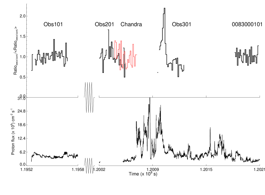
Figure 1: Upper panel: The ratio of the (0.5 keV to 0.7 keV, oxygen emission line band) and (2.5 keV to 5.0 keV, continuum band) lightcurves, scaled to the mean of this ratio for each observation, for observations Obs101, Obs201, and Obs301 along with the next XMM-Newton imaging mode observation that was sufficiently long ($>$4 ks) to be processed (observation id. 0083000101). The same ratio scaling is used for the Chandra data, shown in red. Lower panel: The solar wind proton flux, taken from the ACE SWEPAM instrument.

3 XMM-Newton data analysis

The Science Analysis System (SAS) software (version 8.0.0; http://xmm.esac.esa.int/external/xmm_data_analysis/) was used to process the raw data into calibrated event lists and extract light curves, spectral products and instrument response files. The instrument effective area files were calculated assuming the source flux is extended with no intrinsic spatial structure. The SAS accesses instrument calibration data in so-called current calibration files (CCFs) which are generally updated separately from SAS release versions. In this paper we used the latest public CCFs released as of July 2009.

When creating products from the calibrated event files we applied the following filter expressions in the nomenclature of the SAS; (PATTERN$<$=12)&&(#XMMEA_EM) for the MOS and (PATTERN==0)&&(FLAG==0) for the pn. The specified PATTERN filter selects events within the whole X-ray pattern library for the MOS and mono-pixels only for the pn; as our focus is on detecting line emission below 2 keV, this restriction optimises the energy resolution of the pn with little loss of sensitivity in the energy range of interest. For these event class selections, the energy resolution of the pn is $\sim 70$ eV (FWHM) at 1 keV compared with $\sim 60$ eV in the MOS. The filter #XMMEA_EM removes events from the MOS that are from regions of known bright pixels or columns or near CCD boundaries (which tend to be noisy). The equivalent flag for the pn, #XMMEA_EP, did not remove some residual noisy pixels, but these were removed when we used the more conservative FLAG==0. This flag also masks out events from adjacent regions to noisy pixels.

In addition we selected only events within a radius of 11.7 arcminutes, centred on a communal sky position such that the extraction region of all three cameras was covered by active silicon, barring inter-CCD gaps.

A spectral analysis of the SWCX emission component in Obs301 requires us to identify and account for each of the sources of X-rays that contribute to the combined signal across the field of view. A detailed description of the various components which constitute the XMM-Newton EPIC background is given in Carter & Read (2007). In the following sections we describe how each of these components, plus the contribution from resolved point sources, is either subtracted from our data, or modelled within our spectral fitting. We have used Version 12.5.0 of the XSPEC X-ray spectral fitting package to perform this analysis.

3.1 Resolved point sources

Resolved point sources can potentially contribute a spectrally variable signal and thus need to be removed as far as possible from our datasets. To do this we used the source lists that are automatically produced for the processing of the 2XMM catalogue and are available as a product within the XMM-Newton archive. These lists were used to create an exclusive filter that removed events from the calibrated event lists out to a radius of 35 arcseconds ($\sim 90$% of the on-axis point spread function) from the centre of each source. Using the source count rates within the source lists, we estimate that the total residual resolved source count rate (0.2 to 2.0 keV) in the pn after cleaning would be around $\rm 0.04\,cts\,s^{-1}$ in Obs101. The background subtracted count rate in the same energy band after source removal was $\rm 0.75\ cts\ s^{-1}$, hence, residual sources contribute approximately 5% of the observed diffuse flux in this observation. In Obs301 the diffuse flux count rate is $\rm 1.8\,cts\,s^{-1}$ and the residual contribution from resolved point sources is at around 2%. Figure 2 shows the cleaned images from each camera from Obs301, with the positions of the point sources and spectral extraction region marked, in the energy range 0.3 keV to 2.0 keV. There are 62 sources which overlap the source extraction region.

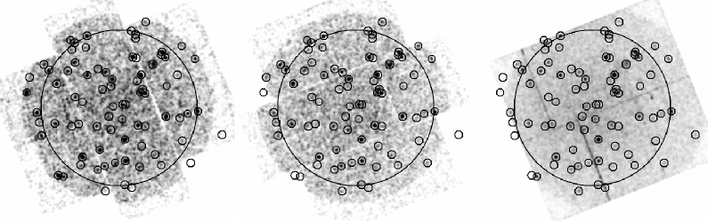
Figure 2: Images from each of the EPIC cameras for Obs301 (left to right); MOS1, MOS2 and pn, in the energy range 0.3 keV to 2.0 keV. The small black circles indicate the point sources removed from analysis, and the large black circle indicates the spatial extraction region used for spectral analysis.

3.2 Soft proton contamination

Soft protons can produce an extremely variable, spectrally smooth, wide-band, whole field of view signal that can be the dominant source of X-rays within an observation. The particles may be solar protons accelerated by reconnection events in the vicinity of the Earth (Lumb et al. 2002). They are funnelled by the telescope mirrors onto the detectors where they are absorbed; the signals produced by individual events are indistinguishable from X-rays. Figure 3 shows the Obs301 2.5 keV to 8.5 keV light curves of the three EPIC cameras (after point-source removal) binned in 100 s intervals. The dataset is extremely contaminated by soft proton flares and show data gaps in the MOS when the instrument was switched to a safe mode. The pn instrument takes longer to setup for a given observation therefore the pn lightcurve starts about 40 minutes after the MOS.

Data cleaning schemes for flares include excluding bins whose count rate in a high energy band exceeds a set threshold or excluding bins which are more than a set value of sigma from the mean value of the light curve. The latter method is that employed by the publicly available Extended Source Analysis Software (ESAS) package, as described in Snowden et al. (2008). At the time of writing the ESAS package is only directly applicable to the MOS data, however, we used the package to derive Good Time Interval (GTI) files for MOS1 and MOS2 and then merged them into a single file which proved to be sufficiently accurate in identifying periods of proton flaring in the pn data.

The data bins accepted by the single GTI file are shown in Figure 3 in black. We have used this data selection for the integrated spectra as described in Section 3.6. We also included the data for the period marked in blue in our analysis of the SWCX lightcurve because we wished to try and establish the start of the period of SWCX enhancement.

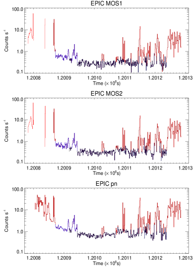
Figure 3: The 2.5 keV to 8.5 keV EPIC lightcurves of the diffuse signal from observation Obs301, incorporating all exposures. The variance in the signal is due to soft proton contamination. Bins marked in red indicate where data have been excluded from further analysis. Bins marked in black are the cleanest data used for spectral fitting of the integrated spectra. Bins in blue are used in addition for analysis of the lightcurve.

Soft protons can have a low temporal variance which is often difficult to detect via an analysis of the lightcurve, although in this case it can be seen that there appears to be a slowly varying signal in the residual GTI periods. This was confirmed as being due to soft protons via our spectral analysis.

The spectral signature of soft protons has been studied by Kuntz & Snowden (2008). These events produce a featureless power-law spectrum unmodified by the detector response. There is generally a correlation between spectral hardness and intensity and the spectral slope can show a break with a steepening at higher energies. The component can be modelled within a typical XSPEC analysis session by folding a power-law (or broken power-law) through a diagonal response matrix (i.e. one constructed to have a response value of 1.0 on the diagonal elements and zero elsewhere). XSPEC Version 12 has the functionality to enable several model spectra to be convolved with distinct responses and then added together into a combined model which can be compared with the data. This combined model refers to the model of the diffuse X-ray emission, which incorporates various background components convolved with the instrument response and the soft proton model convolved with the diagonal response.

3.3 Cosmic-ray particle background (CPB)

High energy cosmic rays produce background either directly within the CCDs or via fluorescence within the spacecraft material surrounding the detectors. This source of background is relatively stable in spectral shape and intensity. The CPB contribution to a given observation can best be estimated by deriving the spectrum from EPIC data taken when the instruments are in the filter wheel closed (FWC) configuration (i.e not open to the sky). In this configuration the observed signal consists of the CPB plus detector noise (Section 3.4). The XMM-Newton Background Working Group (BGWG) maintain co-added event files of FWC data (total exposures of around 700 ksec in each MOS and 300 ksec in the pn) on their public web site .

The CPB spectrum varies across the field of view of each instrument, therefore, it is necessary to extract the spectra from the identical regions to those that define the source spectrum. The spectra so extracted constituted the background files in our XSPEC fits.

It is not unusual for the derived CPB spectrum to require some small amount of re-scaling for a given observation. This can be done by comparing the observed high energy count rate in the source and CPB spectra above an energy where the contribution from components other than the CPB in the source spectrum is expected to be negligible. Naturally, the source dataset must be clean of soft proton contamination before a simple scaling of the CPB can be made. As this was the case in Obs101 and as our model of the diffuse X-ray sky predicted a relatively negligible contribution to the observed count rate in the energy range 7.75 keV to 12.0 keV, we used this band in all three EPIC instruments to derive scaling factors for the CPB of 1.26, 1.11 and 1.08 respectively in the pn, MOS1 and MOS2 (i.e. the observed FWC CPB count rate was greater by these factors than observed in our source observation). Such factors are not uncommon (De Luca & Molendi 2004).

Because our SWCX dominated observation, Obs301, was contaminated by residual soft protons throughout the observation and therefore had a strong contribution from this component at high energies, we were unable to apply the same procedure as for Obs101 to subtract the CPB. We assumed therefore that the scaling factors for the CPB derived from Obs101 would be appropriate for this observation; a reasonable assumption given that the observations are only 6 days apart.

3.4 Detector noise

Detector noise consists of persistent and variable components, in both a temporal and spatial sense. Persistent noise occurs from thermal Poisson processes in each CCD pixel which creates events with sufficient charge to appear above the detector threshold. This component is essentially fixed. It is one component of the signal within filter wheel closed datasets (see Section 3.3) and it is therefore fairly straightforward to subtract from the total signal.

Variable components are primarily due to pixels damaged by radiation. Pixels so bright that they can cause the event rate to exceed the instrument telemetry limit are blocked on board. Other defective areas are recognised by the SAS and events from these regions are flagged (see Section 3), enabling them to be excluded or included depending on the requirements of the analysis.

There are other components, however, that are not so amenable to subtraction via event flagging. CCD5 of the MOS1 detector showed an elevated background across the whole chip characterised by a continuum of spurious events with energies up to $\sim 1$ keV. Our solution was simply to remove this CCD from our analysis. This type of noise signal is variable from observation to observation and other CCDs can also show a similar behaviour with around $\sim 20$% of observations affected at some level (Kuntz & Snowden 2008). The physical cause of the noise is unknown at present.

3.5 Diffuse Galactic and extragalactic emission

Obs101 allowed us to independently derive the contribution from the diffuse Galactic and extragalactic emission components in the direction of Obs301. The target area has a galactic longitude and latitude of ($176^{\circ}$, $40^{\circ}$) so is well away from the plane of the Galaxy and Galactic centre. Having removed the resolved point sources and flare cleaned the data, Obs101 appeared by inspection to contain no evidence for significant residual soft protons or a time varying SWCX component. We therefore assumed that the resultant diffuse emission comes from non-varying sources and that the spectrum and intensity of this component could be fixed and applied to observation Obs301.

Following previous authors (e.g. Galeazzi et al. (2007)) we have modelled the Obs101 diffuse photon emission with a three component description. The first component is a constant un-absorbed plasma representing emission from the local hot bubble and a possible contribution from SWCX emission at the boundary of the heliosphere (Robertson & Cravens 2003a; Koutroumpa et al. 2007). Any contribution from the heliospheric SWCX we assume to be essentially constant over the 6 days between the observations. The second component is an absorbed plasma representing emission from the Galactic halo. We used the APEC (Smith et al. 2001) model within XSPEC to model the plasma components although the commonly used alternative Mekal and Raymond-Smith models gave statistically identical results. The third component, also absorbed by the same line of sight material, is a power law representing the unresolved extragalactic X-ray background from point sources. For the absorption, we have used the phabs model within XSPEC. The element abundances in the absorption and emission models used were those set by the wilm table (Wilms et al. 2000). The value of $\rm N_{H}$ was fixed at the Galactic line of sight value of $\rm 2.79\times 10^{20}\ cm^{2}$ and derived using the nH tool available from the HEASARC .

We first independently fit the model to each of the CPB background subtracted Obs101 spectra from the pn, MOS1 and MOS2. However, after several analysis iterations we found that we could achieve an acceptable fit to the data by jointly fitting the model to all three cameras allowing only the global normalisation of the entire model to vary between the cameras. Table 2 lists the derived model parameters and component fluxes. The fluxes from each camera are consistent with each other at the 90% confidence level, although the MOS returns values $\sim 20$% lower than the pn.

Figure 4 shows the data compared to the best-fit model in each of the three cameras. When fitting the data we excluded the energy range 1.35 keV to 1.9 keV because, as can been seen in the figure, the strong instrumental Al $\rm K_{\alpha}$ and Si $\rm K_{\alpha}$ lines can produce large residuals at these energies after background subtraction. There is also a broad residual in the pn fit at 0.45 keV whose strength is not sensitive to the particulars of which abundance table or plasma model within XSPEC is selected. MOS1 has a similar, although narrower feature, whereas MOS2 does not. The strength of the feature is not sufficient to have a significant bearing on our analysis of the SWCX signal within Obs301.

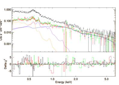
Figure 4: Background subtracted pn (black), MOS1 (red) and MOS2 (green) spectra from Obs101 compared with a model of the diffuse sky emission. Also shown are the three components of the model, the un-absorbed plasma (orange), the absorbed plasma (purple) and absorbed power-law continuum (blue). For clarity, only the individual model components for MOS1 are shown. The lower panel shows the deviation of the data from the model.

Table 2: Sky model parameters in the direction of Obs301 derived from an analysis of Obs101. Quoted errors are 90% confidence for one interesting parameter. Fluxes are observed values in the energy range 0.2 keV to 10 keV in units of $\rm 10^{-8}\,ergs\,cm^{-2}\,s^{-1}\,sr^{-1}$.

Diffuse Sky Background Model
Reduced $\chi^{2}$ / Degrees of Freedom		0.99 / 1008
Component	Parameter/Flux	Value (Error)
Unabs. Plasma	Temperature (keV)	0.11 (0.01)
	MOS1 Flux	2.04 (0.18)
	MOS2 Flux	1.99 (0.18)
	pn Flux	2.42 (0.20)
Abs. Plasma	Temperature (keV)	0.23 (0.02)
	MOS1 Flux	1.23 (0.18)
	MOS2 Flux	1.12 (0.18)
	pn Flux	1.46 (0.21)
Abs. CXRB	Photon Index	1.44 (0.12)
	MOS1 Flux	5.31 (0.56)
	MOS2 Flux	5.18 (0.55)
	pn Flux	6.29 (0.63)

3.6 Solar Wind Charge Exchange X-ray Emission

The lightcurve of Obs301 in Figure 1 suggests the soft band flux has a flare and a quiescent period. Background subtracted spectra integrated over these intervals (extracted from the soft proton flare-cleaned data) are shown in Figure 5. In addition we show the diffuse sky model folded through the instrument response and the strong residual soft proton component. The soft protons are modelled with a single power law spectrum fit by initially restricting the spectral fit to the range 2.5 keV to 6.5 keV. The extrapolation of the power law shows that the soft proton component is comparable to or weaker than the non-variable diffuse sky component below $\sim 1$ keV, and may be weaker still because, as previously discussed, soft protons often display a spectral break. For this reason, the strength of the residual SWCX component at low energies may be underestimated by a few percent.

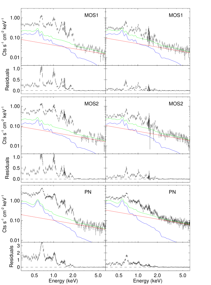
Figure 5: Obs301 background-subtracted spectra integrated from $\rm T=1.200918\times 10^{8}\,s\ to\ 1.201035\times 10^{8}\,s$ (left panels) and from $\rm T=1.201035\times 10^{8}\,s\ to\ 1.201230\times 10^{8}\,s$ (right panels). Contributions are shown from soft protons (red), the non-variable diffuse sky background (blue), and these components combined (green). The variable excess flux, seen in the lower panels, is due to SWCX.

It is evident from Figure 5 that both the flare and quiescent periods show an excess flux above the combined diffuse sky flux and soft proton contribution which is spectrally distinct from these components. The excess clearly contains emission lines and is variable which are both signatures of SWCX. The most prominent lines are at 0.65 keV and 1.02 keV which we identify with O VIII and Ne X. Laboratory measurements and theoretical calculations of SWCX emission (e.g. Wargelin et al. (2008)) indicate that emission spectra will contain multiple lines from a variety of ions and their transitions, most of which will be unresolved in the EPIC instruments, given the limits of the energy resolution of the detectors.

Our spectral model of the SWCX excess was built up from a series of zero width Gaussians with energies fixed at known X-ray emission transitions from likely solar wind ions. For CV, CVI, NVI, NVII, O VII and O VIII we have used the theoretical model by Bodewits (2007) (Table 8.2), who has calculated the relative emission cross-sections of these bare and H-like ions (their state before electron capture) in collision with atomic hydrogen for a variety of solar wind velocities. We have used the tabulated values for a velocity of $\rm 600\ km\ s^{-1}$ which is close to the velocity measured by ACE at this epoch. Our model fitting allowed the six normalisations of the principal transition from each of these ions to be free, but constrained the normalisations of the weaker transitions to the ratios predicted by the Bodewits’ model. In all, these ions contributed 33 lines between 0.299 keV and 0.849 keV.

At higher energies we have taken a more empirical approach by adding sufficient lines at known transition energies to characterise the bulk of the residual excess emission. This will be an incomplete list due to the multiple transitions expected from Fe. Table 3 lists the principal transitions we have included in the SWCX model.

We have fit our combined model (containing the SWCX, sky background and soft proton components) jointly to the integrated spectra from each of the EPIC cameras. The free parameters in the fit are the normalisations of the principal ions in the SWCX model plus global normalisations applied to the individual MOS spectra (the pn global normalisation was fixed at 1.0).

In Table 3 we list the flux of the O VIII line at 0.65 keV and the ratio of the fluxes for each of the other ions to O VIII, and the total flux of the SWCX model. As with our analysis of the diffuse sky background in Obs101, the broad-band MOS fluxes are lower than that measured by the pn by a similar factor.

In a study of the inter-calibration of point sources from the 2XMM catalogue, Mateos et al. (2009) found the reverse trend; on average the MOS cameras register a higher flux than the pn by 7-9% below 4.5 keV. We can only attribute the difference to some unknown calibration uncertainty in the calculation of the effective area for point sources compared with an extended region.

Figure 6 shows the best fit SWCX spectral model (plus the non-variable diffuse sky and variable soft proton components combined) to the background-subtracted and flare-cleaned pn spectrum. The non-Gaussian shape of the pn detector response (the MOS is similar; the Gaussian shape is distorted by a low-energy shoulder) is evident from the principal O VIII line.

The temporal variation in the SWCX emission has been mapped by extracting spectra in eight 2 ks intervals followed by five 4 ks intervals. This covers the soft proton flare-cleaned period plus the additional segment as shown in Figure 3. For each interval, we show in Figure 7 the fitted fluxes of the O VIII (0.653 keV) line and the ratio of the fluxes of OVII (0.561 keV), Ne X (1.022 keV), Mg XI (1.329  keV) and Si XIV (2.000 keV) to OVIII. There is little evidence for a significant compositional change throughout the observation with the possible exception of the second and third bins where the flux ratios of the heavier ions are somewhat higher compared to the average.

Ion compositional data (level 2, hourly averaged) from the SWICS/SWIMS instrument on board ACE (Gloeckler et al. 1998) are sparse for the period of interest. XMM-Newton therefore is able in this case to provide supplementary abundance information where ACE, for data quality reasons, cannot.

Table 3: Measured fluxes in the SWCX spectral model. Here we list only the principal transitions from C, N and O plus the additional selected transitions from Ne, Mg, Si and Fe. The figure for O VIII is the measured flux in units of $\rm 10^{-8}\ ergs\ cm^{-2}\ s^{-1}\ sr^{-1}$. The remainder of the table is the ratio of the measured flux for that ion to O VIII and the total flux of the SWCX model.

Ion	Principal Energy (keV)	Ion Ratio / OVIII Flux
C V	0.299	0.50(0.16)
C VI	0.367	0.28(0.08)
N VI	0.420	0.06(0.05)
N VII	0.500	0.19(0.03)
O VII	0.561	0.12(0.03)
O VIII	0.653	2.70(0.09)
Fe XVII	0.73	0.13(0.01)
Fe XVII	0.82	0.05(0.02)
Fe XVIII	0.87	0.10(0.03)
Fe XIX/Ne IX	0.92	0.14(0.03)
Fe XX	0.96	0.09(0.02)
Ne X	1.022	0.46(0.02)
Fe??/Ne IX	1.10	0.20(0.01)
Fe XX/Ne X	1.22	0.08(0.01)
Mg XI	1.33	0.28(0.01)
Mg XII	1.47	0.29(0.02)
Mg XI	1.60	0.06(0.01)
Al XIII	1.73	0.08(0.01)
Si XIII	1.85	0.30(0.02)
Si XIV	2.00	0.15(0.02)
Total SWCX (pn normalisation = 1.0)		12.58 (0.20)
MOS1 Normalisation		0.80 (0.02)
MOS2 Normalisation		0.92 (0.02)
Reduced $\chi^{2}$ / Degrees of Freedom		1.17 / 1546

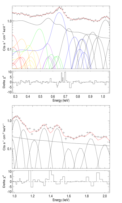
Figure 6: The SWCX spectral model fitted to the integrated background subtracted and flare-cleaned pn spectrum of Obs301. The top panel is the spectrum from 0.275 keV to 1.055 keV and the bottom panel is the spectrum from 0.975 keV to 2.055 keV. The sum of the non-variable sky and variable soft proton components is the continuous line in black. The lines due to C, N and O are colour coded; C V (red), C VI (orange), N VI (yellow), N VII (green), O VII (purple) and O VIII (blue). Heavier elements are in black. The residual at $\sim 1.4$ keV may be due to incomplete background subtraction at the energy of the strong $\rm Al\ K_{\alpha}$ instrumental line.

Figure 7: Lightcurves of selected ions from Obs301. The top panel is the OVIII flux in units of $\rm 10^{-8}\ ergs\,cm^{-2}\,s^{-1}\,sr^{-1}$. Lower panels are the ratio of the flux of the selected ion to OVIII.

4 Viewing geometry and orientation of XMM-Newton

The expected X-ray emissivity of SWCX emission from the solar wind interaction with the magnetosheath can be estimated from the integrated emission along the line of sight for the observer.

The emissivity expected (Cravens 2000) is given by the expression:

$$P_{{}^{\chi}}=\alpha\eta_{{}^{SW}}\eta_{{}^{n}}\langle g\rangle\ eVcm{{}^{-3}}s{{}^{-1}}$$ (1)

where $\alpha$ is a scale factor dependent on various aspects of the charge exchange such as the interaction cross-section and the abundances of the solar wind ions, $\eta_{{}^{SW}}$ is the density of the solar wind protons, $\eta_{{}^{n}}$ is the density of the neutral species and $\langle g\rangle$ is their relative velocity.

The flux is given by integrating along a particular line of sight:

$$F=\frac{1}{4\pi}\int_{0}^{\infty}P_{{}^{\chi}}ds\ ph\ cm{{}^{-2}}s{{}^{-1}}sr{{}^{-1}}$$ (2)

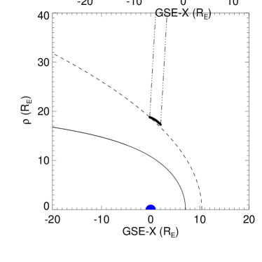
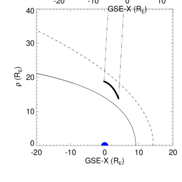
Figure 8: Obs301 XMM-Newton positions, in the ecliptic plane, progressing (top to bottom) from T=1.200805$\rm\times 10^{8}\,s$ to T=1.2009$\rm\times 10^{8}\,s$, through T=1.2010$\rm\times 10^{8}\,s$ until T=1.2012$\rm\times 10^{8}\,s$. On the y-axis is $\rho$, as defined by $\rm\sqrt{GSE\mathchar 45\relax Y^{2}+GSE\mathchar 45\relax Z^{2}}$, plotted against the GSE-X coordinate. The solid and dashed lines give the locations of the magnetopause and bow shock at the end of each period. The dot-dot-dashed lines show the line of sight of XMM-Newton.

To assist in our analysis for this section, we took data from the Solar Wind Experiment (SWE) instrument on board the spacecraft Wind (Ogilvie et al. 1995) and data as measured by the SWEPAM instrument of ACE.

In Figure 8, we plot the position of XMM-Newton and the magnetopause and bow shock boundaries and the line of sight during Obs301. The line of sight pointed through the flanks of the magnetosheath throughout the observation. XMM-Newton crossed the bow shock boundary as it moved along its orbit, and as the boundary position changes in response to conditions in the solar wind. The magnetopause and bow shock locations may vary dramatically, especially under extreme solar wind conditions as we see in this case. We used the model of Shue et al. (1998), which takes the strength of one component of the magnetic field ($B_{z}$) and the proton dynamic pressure as input, to calculate the location of the magnetopause. The position of the bow shock stand-off distance (the distance from the Earth to the bow shock on the Earth-Sun line) is calculated using the solar wind dynamic pressure (Khan & Cowley 1999), and its shape is approximated using a simple parabola (eccentricity 0.81). We plot the positions of XMM-Newton as it moves from T=1.200805$\times 10^{8}\,s$ to T=1.2009$\times 10^{8}\,s$ (top), through T=1.2010$\times 10^{8}\,s$ (middle) until T=1.2012$\times 10^{8}\,s$. The magnetopause and bow shock positions are plotted for the end of each period. XMM-Newton remains outside the magnetopause for the entirety of the observation, but may cross the bow shock boundary when the magnetosheath is compressed in response to the solar wind (middle panel). Therefore the line of sight through the magnetosheath region is short, but not zero, at various times during Obs301.

During Obs301 the average solar proton density (level 2, hourly averaged data from ACE), was measured as $\rm 13\,cm^{-3}$ and had an average speed of $\rm 647\,km\,s^{-1}$. Exospheric neutral hydrogen densities fall off as $\rm R_{E}$^-3 and are normalised to a value of $\rm 25\,cm^{-3}$ at a distance of 10 $\rm R_{E}$ (Hodges 1994; Cravens et al. 2001). Using Equation 2 and the solar wind parameters above, we wished to estimate the expected X-ray emission seen by XMM-Newton at its average distance from Earth of 13.8 $\rm R_{E}$, integrating out to 100 $\rm R_{E}$. By this method we compare the scale of the emission as recorded by XMM-Newton to a non-time resolved order of magnitude estimation for the expected X-ray emission.

The solar wind slows down and its density increases inside the magnetosheath. The magnetosheath is the region between the bow shock (where the solar wind slows down from supersonic to subsonic speeds) and magnetopause (the boundary layer separating the plasma of the solar wind and that of the Earth’s magnetic field). In this estimation, we base the starting point at the average distance of XMM-Newton from Earth, so that the line of sight through the magnetosheath region is short compared to the remaining line of sight out to a maximum of 100 $\rm R_{E}$. We approximate a line of sight of 2.2 $\rm R_{E}$ from the average position of XMM-Newton to the bow shock boundary, with the remainder of the line of sight intersecting unperturbed solar wind. To approximate these changes, we scaled hydrodynamical models of Spreiter et al. (1966) (Kuntz, private communication) to the magnetopause standoff distance of 8 $\rm R_{E}$ and extract factors for adjusting the solar wind parameters at the relevant position within the magnetosheath. We increase the solar wind density by a factor of 3.5 and reduce the solar wind speed by a factor of 0.8 within the magnetosheath region only, and leave it undisturbed outside the bow shock.

The value of $\alpha$ is dependent on the abundances of the ion species contributing to the charge exchange process, along with the cross-section and energy of each interaction in the energy band of interest. For this estimation we consider only contributions from the O VII and O VIII. SWCX emission is directly proportional to $\alpha$, which is in turn proportional to the abundance of the ion specie in question. We use the ratio of OVII to OVIII flux from our spectral analysis in Section 3.6, the cross-sections found in Bodewits (2007) (assuming a solar wind with velocity $\rm 600\,km\,s^{-1}$) and an oxygen to hydrogen ratio of 1/1780 as given in Schwadron & Cravens (2000) to derive an OVII to OVIII abundance ratio of 0.085:0.915. We then calculate $\alpha$ for these two ion species to be $\rm 2.3\times 10^{-15}\,eV\,cm^{2}$. Although the solar wind speeds during Obs301 are more common of a fast solar wind state, CMEs are enriched with high oxygen charge states and other minor ions (Richardson & Cane 2004).

The total expected (oxygen band) X-ray emission along the line of sight and for average solar wind conditions was estimated to be $\rm 9.5\,keV\,(1.5\times 10^{-8}\,ergs)\,cm^{-2}\,s^{-1}\,sr^{-1}$. The contribution from inside the magnetosheath is estimated to be $\rm 4.8\,keV\,(7.6\times 10^{-9}\,ergs)\,cm^{-2}\,s^{-1}\,sr^{-1}$ which represents approximately 50% of the total. From our spectral analysis, we observe a flux of $\sim\rm 18.9\,keV\,(\sim 3.02\times 10^{-8}\,ergs)\,cm^{-2}\,s^{-1}\,sr^{-1}$ from the O VII and O VIII emission lines, approximately 2 times greater than we estimate, but which is consistent given the various assumptions as detailed above. For example, the density of the plasma outside the bow shock may be even higher than the values used in this calculation, due to turbulent processes, localised density enhancements and/or the anisotropic distribution of neutral atoms in the vicinity of the Earth (Hodges 1994).

Higher levels of geocoronal SWCX emission would be expected had XMM-Newton been observing a target that required a pointing vector that intercepted the area of highest X-ray emission, namely around the subsolar point, defined as the position of the magnetopause on the sunward side of the Earth-Sun line (Robertson & Cravens 2003a; Robertson et al. 2006). The solar wind flux during Obs301 was so high that the magnetopause was pushed close to the Earth as a result of the balance between the pressure of the solar wind and that of the Earth’s magnetic field. Therefore, only a very short line of sight of XMM-Newton intersected the magnetosheath region for a large proportion of the observation. The remainder of the line of sight intersected undisturbed solar plasma. There was a sufficient density of neutral donor atoms outside of the bow shock, interacting with a particularly dense solar plasma, that a significant contribution to the SWCX signal originated from this region, even though beyond the bow shock the solar wind has not been slowed considerably or the density increased as it would have been within the magnetosheath. The SWCX emission in this case was emitted from both before and just beyond the bow shock boundary. Clearly in cases where XMM-Newton does not have an optimal view through the magnetosheath, there is the possibility of detecting SWCX emission from the local region.

In Figure 9 we plot the ACE and Wind proton density lightcurves. We include on the plot the combined XMM-Newton EPIC instrument flare-filtered lightcurve, between 0.5 keV and 0.7 keV. The EPIC lightcurve shows the same general temporal behaviour as the enhancements in solar proton density measured by both ACE and Wind.

The offset in time between the signals at ACE and Wind is explained by the separation between the solar wind monitoring spacecraft. We are unable to determine the moment when the signal first crossed into the field of view of XMM-Newton, as the XMM-Newton data had to be heavily filtered for soft proton contamination at the beginning of the observation. The shape of the lightcurve seen by Wind is not exactly the same as that seen by ACE, so we infer that some evolution of the CME may be occurring or that there are local inhomogeneities within the CME wavefront although the bulk movement is fairly constant. The shape of the XMM-Newton lightcurve suggests some level of averaging along the XMM-Newton line of sight and it must be kept in mind that the proton density is only a proxy for the ion composition of the solar wind. From the positions of the spacecraft we are able to ascertain that the CME wavefront extends at least 25 $\rm R_{E}$ in the GSE-Y direction. We have shown that SWCX emission is non-zero throughout the XMM-Newton observation, however we assume that the major bulk of the CME has passed by a time at T=1.2012$\times 10^{8}\,s$. If we take the start of the CME wavefront to be at approximately T=1.20085$\times 10^{8}\,s$ travelling at an average speed of $\rm 647\,km\,s^{-1}$, the CME extends a minimum of 3500 $\rm R_{E}$ in the GSE-X direction.

Figure 9: ACE and Wind solar proton densities plus XMM-Newton combined EPIC instrument (0.5 keV to 0.7 keV, oxygen emission line band) lightcurve (panels top to bottom). The XMM-Newton lightcurve has been flare-filtered using the method described in the text.

As the solar proton density lightcurves from both ACE and Wind showed the same shape we conclude that the same density enhancement was received at both these solar wind monitors and subsequently XMM-Newton. We assume a planar wavefront for the enhancement, which is a reasonable assumption at a distance of 1 AU for a CME (Zurbuchen & Richardson 2006). Following a similar analysis to that of Collier et al. (2005) and Collier et al. (1998) the orientation of the passing wavefront could be derived using the delay between the signal received at ACE and that received by Wind. Using a discrete correlation function algorithm (Edelson & Krolik 1988) between the ACE and Wind proton density lightcurves (Figure 9), based on the period of the solar proton density enhancement between T=1.2009$\times 10^{8}\,s$ and T=1.2011$\times 10^{8}\,s$, we find a delay of 26$\pm$1 minutes from ACE to Wind. For a wave front travelling perpendicular to the Earth-Sun line at the average speed mentioned above, this results in a delay time of 29 minutes from ACE to Wind. The difference in delay times suggests that a tilted wave front at approximately 40 degrees would have passed in the vicinity of the Earth and XMM-Newton. In Figure 10 we plot the position of ACE, Wind and XMM-Newton at T=1.2009$\times 10^{8}\,s$ of Obs301.

Figure 10: XMM-Newton, ACE and Wind positions at the time of Obs301, in GSE-coordinates in the ecliptic plane. Positions in brackets are in $\rm R_{E}$. The position of the magnetopause, as calculated using the Shue et al. (1998) model, is shown for the start of Obs301. The dashed lines are used to aid visualisation and the wavefront is represented by the tilted solid lines.

5 Discussion and conclusions

We consider the possibility that the SWCX enhancement of Obs301 is linked to the CME event of the 19th October 2001 (Wang et al. 2005). The delay between the occurrence of the CME at the solar corona and its arrival near Earth would be approximately two and a half days. Increased solar proton fluxes were registered by both ACE and Wind and therefore this plasma cloud would have passed in the immediate vicinity of the Earth. It is not always the case that enhancements in solar proton fluxes, and any accompanying highly charged ions, are registered by increased incidents of soft proton flaring or SWCX enhancements by XMM-Newton. However, the arrival of the peak of the low energy enhancement as seen by XMM-Newton is consistent with the delay expected as the feature passes in sequence from ACE to Wind, on to a region intersected by the line of sight of XMM-Newton.

We have shown that line emission from O VIII is very prominent and dominates that of O VII, contrary to signatures of heliospheric SWCX (Koutroumpa et al. 2009). We have also shown in our spectral analysis, that the observed flux from SWCX emission is much greater than that from a simple estimate of the expected emission, based on the abundances of a slow solar wind. Also, mid-energy emission lines in the regime 0.70 keV to 2.00 keV infer the presence of highly charged states of iron, as is often seen in a CME (Zurbuchen & Richardson 2006; Zhao et al. 2007). We see no significant compositional changes in the line emission over the duration of the XMM-Newton observation. In addition, we have observed emission at 2.00 keV from highly charged states of silicon, implying a very high temperature plasma. A CME, rather than a steady state solar wind, would explain the large enhancements, flux observed and the richness of the spectrum as seen by XMM-Newton. This case is the richest spectrally of those examined by Carter & Sembay (2008).

CMEs have been used to explain the results of other X-ray observations in the literature pertaining to the diffuse X-ray background. Henley & Shelton (2008) invoked a CME to explain differences between results obtained from XMM-Newton and Suzaku, when determining Halo and Local Bubble X-ray spectra. They also observed emission from Mg XI and Ne IX, although emission lines from oxygen were less significant. They attribute this emission to a possible localised enhancement in solar wind density crossing the line of sight of XMM-Newton. Smith et al. (2005) attributed the anomalously high level of O VIII seen in their observation of a nearby molecular cloud to SWCX, and noted this was unlikely to be due to SWCX from a steady state solar wind. Instead they conclude that their enhancement was due to charge exchange from a CME and the interstellar medium, probably at a distance of a few AU from the Sun, due to the depletion of neutral gas available for charge exchange near the Sun. We eliminate the possibility that the emission seen in Obs301 is due to SWCX occurring at the heliospheric boundary or at a large distance from Earth. Short-term variations can occur for heliospheric SWCX, especially if observing along the helium focusing cone (Robertson & Cravens 2003a, b), but the pointing of XMM-Newton  which does not insect the region of peak emission from this area, argues against this case. In addition, the abundant emission line spectrum and the variations in the fluxes of the major ions in the spectrum which reflect the variations in solar proton flux support a geocoronal occurrence of SWCX. We conclude that the SWCX interaction we have observed occurs between ions from a CME and neutrals in the exosphere of the Earth, at a relatively close distance to the Earth, but not confined to the magnetosheath within the bow shock.

Although data regarding the ion states of the solar wind for the period of Obs301 from the solar wind monitors ACE and Wind are sparse, we have been able to identify ions from a rich set of emission lines from a passing CME. Not all CMEs detected by ACE will be detected by Wind, or indeed intersect the line of sight of XMM-Newton. XMM-Newton was not optimised to study the magnetosheath or near Earth regions. However, we have shown that XMM-Newton can be used to provide additional compositional information of the solar wind plasma, especially for the highest charge state ions, to that obtained by upstream solar wind monitors, providing the observing geometries and inclinations of the incoming wave fronts are favourable.

References

- Acuña et al. (1995) Acuña M. H., Ogilvie K. W., Baker D. N., Curtis S. A., Fairfield D. H., Mish W. H., 1995, Space Science Reviews, 71, 5
- Bodewits (2007) Bodewits D., 2007, PhD thesis, University of Groningen, P.O. Box 72, 9700 AB Groningen, The Netherlands
- Carter & Read (2007) Carter J. A., Read A. M., 2007, A&A, 464, 1155
- Carter & Sembay (2008) Carter J. A., Sembay S., 2008, A&A, 489, 837
- Collier et al. (2008) Collier M. R., Carter J., Cravens T., Hills H. K., Kuntz K., Porter F. S., Read A., Robertson I., Sembay S., Snowden S. L., Stubbs T., Travnicek P., 2008, LPI Contributions, 1415, 2082
- Collier et al. (2005) Collier M. R., Moore T. E., Snowden S. L., Kuntz K. D., 2005, Advances in Space Research, 35, 2157
- Collier et al. (1998) Collier M. R., Slavin J. A., Lepping R. P., Szabo A., Ogilvie K., 1998, Geophys. Res. Lett., 25, 2509
- Cravens (2000) Cravens T. E., 2000, ApJL, 532, L153
- Cravens et al. (2001) Cravens T. E., Robertson I. P., Snowden S. L., 2001, J. Geophys. Res., 106, 24883
- De Luca & Molendi (2004) De Luca A., Molendi S., 2004, A&A, 419, 837
- Domingo et al. (1995) Domingo V., Fleck B., Poland A. I., 1995, Space Science Reviews, 72, 81
- Edelson & Krolik (1988) Edelson R. A., Krolik J. H., 1988, ApJ, 333, 646
- Galeazzi et al. (2007) Galeazzi M., Gupta A., Covey K., Ursino E., 2007, ApJ, 658, 1081
- Gloeckler et al. (1998) Gloeckler G., Cain J., Ipavich F. M., Tums E. O., Bedini P., Fisk L. A., Zurbuchen T. H., Bochsler P., Fischer J., Wimmer-Schweingruber R. F., Geiss J., Kallenbach R., 1998, Space Science Reviews, 86, 497
- Henley & Shelton (2008) Henley D. B., Shelton R. L., 2008, ApJ, 676, 335
- Hodges (1994) Hodges R. R. J., 1994, J. Geophys. Res., 99, 23229
- Jansen et al. (2001) Jansen F., Lumb D., Altieri B., Clavel J., Ehle M., Erd C., Gabriel C., Guainazzi M., Gondoin P., Much R., Munoz R., Santos M., Schartel N., Texier D., Vacanti G., 2001, A&A, 365, L1
- Khan & Cowley (1999) Khan H., Cowley S. W. H., 1999, Annales Geophysicae, 17, 1306
- Koutroumpa et al. (2007) Koutroumpa D., Acero F., Lallement R., Ballet J., Kharchenko V., 2007, A&A, 475, 901
- Koutroumpa et al. (2009) Koutroumpa D., Lallement R., Kharchenko V., Dalgarno A., 2009, Space Science Reviews, 143, 217
- Kuntz & Snowden (2008) Kuntz K. D., Snowden S. L., 2008, A&A, 478, 575
- Lumb et al. (2002) Lumb D. H., Warwick R. S., Page M., De Luca A., 2002, A&A, 389, 93
- Mateos et al. (2009) Mateos S., Saxton R. D., Read A. M., Sembay S., 2009, A&A, 496, 879
- McComas et al. (1998) McComas D. J., Bame S. J., Barker P., Feldman W. C., Phillips J. L., Riley P., Griffee J. W., 1998, Space Science Reviews, 86, 563
- Ogilvie et al. (1995) Ogilvie K. W., Chornay D. J., Fritzenreiter R. J., Hunsaker F., et al., 1995, Space Science Reviews, 71, 55
- Richardson & Cane (2004) Richardson I. G., Cane H. V., 2004, Journal of Geophysical Research (Space Physics), 109, 9104
- Robertson et al. (2006) Robertson I. P., Collier M. R., Cravens T. E., Fok M.-C., 2006, Journal of Geophysical Research (Space Physics), 111, 12105
- Robertson & Cravens (2003a) Robertson I. P., Cravens T. E., 2003a, Journal of Geophysical Research (Space Physics), 108, 8031
- Robertson & Cravens (2003b) Robertson I. P., Cravens T. E., 2003b, Geophys. Res. Lett., 30, 080000
- Schwadron & Cravens (2000) Schwadron N. A., Cravens T. E., 2000, ApJ, 544, 558
- Shue et al. (1998) Shue J.-H., Song P., Russell C. T., Steinberg J. T., Chao J. K., Zastenker G., Vaisberg O. L., Kokubun S., Singer H. J., Detman T. R., Kawano H., 1998, J. Geophys. Res., 103, 17691
- Smith et al. (2001) Smith R. K., Brickhouse N. S., Liedahl D. A., Raymond J. C., 2001, ApJL, 556, L91
- Smith et al. (2005) Smith R. K., Edgar R. J., Plucinsky P. P., Wargelin B. J., Freeman P. E., Biller B. A., 2005, ApJ, 623, 225
- Snowden et al. (2004) Snowden S. L., Collier M. R., Kuntz K. D., 2004, ApJ, 610, 1182
- Snowden et al. (2008) Snowden S. L., Mushotzky R. F., Kuntz K. D., Davis D. S., 2008, A&A, 478, 615
- Spreiter et al. (1966) Spreiter J. R., Summers A. L., Alksne A. Y., 1966, P&SS, 14, 223
- Stone et al. (1998) Stone E. C., Frandsen A. M., Mewaldt R. A., Christian E. R., Margolies D., Ormes J. F., Snow F., 1998, Space Science Reviews, 86, 1
- Turner et al. (2001) Turner M. J. L., Abbey A., Arnaud M., Balasini M., et al., 2001, A&A, 365, L27
- Wang et al. (2005) Wang X., Wurz P., Bochsler P., Ipavich F., Paquette J., Wimmer-Schweingruber R. F., 2005, in Dere K., Wang J., Yan Y., eds, Coronal and Stellar Mass Ejections Vol. 226 of IAU Symposium, Effect of Coronal Mass Ejection Interactions on the SOHO/CELIAS/MTOF Measurements. pp 409–413
- Wargelin et al. (2008) Wargelin B. J., Beiersdorfer P., Brown G. V., 2008, Canadian Journal of Physics, 86, 151
- Weisskopf et al. (2000) Weisskopf M. C., Tananbaum H. D., Van Speybroeck L. P., O’Dell S. L., 2000, in Truemper J. E., Aschenbach B., eds, Society of Photo-Optical Instrumentation Engineers (SPIE) Conference Series Vol. 4012 of Society of Photo-Optical Instrumentation Engineers (SPIE) Conference Series, Chandra X-ray Observatory (CXO): overview. pp 2–16
- Wilms et al. (2000) Wilms J., Allen A., McCray R., 2000, ApJ, 542, 914
- Zhao et al. (2007) Zhao L., Zurbuchen T., Fisk L., 2007, AGU Fall Meeting Abstracts, pp A276+
- Zurbuchen & Richardson (2006) Zurbuchen T. H., Richardson I. G., 2006, Space Science Reviews, 123, 31