Turbulence without Richardson-Kolmogorov cascade

$\mbox{N. Mazellier}^{1}$ $\mbox{ \& J.C. Vassilicos}^{1,2}$

$\mbox{}^{1}$Turbulence, Mixing and Flow Control Group, Department of Aeronautics
$\mbox{}^{2}$Institute for Mathematical Sciences
Imperial College London, London, SW7 2BY, UK

Abstract

We investigate experimentally wind tunnel turbulence generated by multiscale/fractal grids pertaining to the same class of low-blockage space-filling fractal square grids. These grids are not active and nevertheless produce very much higher turbulence intensities $u^{\prime}/U$ and Reynolds numbers $Re_{\lambda}$ than higher blockage regular grids. Our hot wire anemometry confirms the existence of a protracted production region where turbulence intensity grows followed by a decay region where it decreases, as first reported by Hurst & Vassilicos [15]. We introduce the wake-interaction length-scale $x_{*}$ and show that the peak of turbulence intensity demarcating these two regions along the centreline is positioned at about $0.5x_{*}$. The streamwise evolutions on the centreline of the streamwise mean flow and of various statistics of the streamwise fluctuating velocity all scale with $x_{*}$. Mean flow and turbulence intensity profiles are inhomogeneous at streamwise distances from the fractal grid smaller than $0.5x_{*}$, but appear quite homogeneous beyond $0.5x_{*}$. The velocity fluctuations are highly non-gaussian in the production region but approximately gaussian in the decay region. Our results confirm the finding of Seoud & Vassilicos [31] that the ratio of the integral length-scale $L_{u}$ to the Taylor microscale $\lambda$ remains constant even though the Reynolds number $Re_{\lambda}$ decreases during turbulence decay in the region beyond $0.5x_{*}$. As a result the scaling $L_{u}/\lambda\sim Re_{\lambda}$ which follows from the $u^{\prime 3}/L_{u}$ scaling of the dissipation rate in boundary-free shear flows and in usual grid-generated turbulence does not hold here. This extraordinary decoupling is consistent with a non-cascading and instead self-preserving single-length scale type of decaying homogeneous turbulence proposed by George & Wang [12], but we also show that $L_{u}/\lambda$ is nevertheless an increasing function of the inlet Reynolds number $Re_{0}$. Finally, we offer a detailed comparison of the main assumption and consequences of the George & Wang theory against our fractal-generated turbulence data.

1 Introduction

Which turbulence properties are our current best candidates for universality or, at least, for the definition of universality classes? The assumed independence of the turbulence kinetic energy dissipation rate on Reynolds number Re in the high Re limit is a cornerstone assumption on which Kolmogorov’s phenomenology is built and on which one-point and two-point closures and LES rely, whether directly or indirectly [34], [9], [29], [30], [21]. This cornerstone assumption is believed to hold universally (at least for relatively weakly strained/sheared turbulent flows). It is also related to the universal tendency of turbulent flows to develop sharp velocity gradients within them and to the apparently universal geometrical statistics of these gradients [32], as to the apparently universal mix of vortex stretching and compression (described in some detail by Tsinober [35] who introduced the expression “qualitative universality" to describe such ubiquitous qualitative properties).

Evidence against universality has been reported since the 1970s, if not earlier, in works led by Roshko, Lykoudis, Wygnanski, Champagne and George (see for example [11] and references therein as well as the landmark work of Bevilaqua & Lykoudis [5] and more recent works such as [36] and [20] to cite but a few) and has often been accounted for by the presence or absence of long-lived coherent structures. Coherent/persistent flow structures can actually appear at all scales and can be the carrier of long-range memory, thus implying long-range effects of boundary/inlet conditions.

In summary, kinetic energy dissipation, vortex stretching and compression, geometrical alignments, coherent structures and the universality or non-universality of each one of these properties are central to turbulent flows with an impact which includes engineering turbulence modelling and basic Kolmogorov phenomenology and scalings. Is it possible to tamper with these properties by systematic modifications of a flow’s boundary and/or inlet/upstream conditions?

To investigate such questions, new classes of turbulent flows have recently been proposed which allow for systematic and well-controlled changes in multiscale boundary and/or upstream conditions. These new classes of flows fall under the general banner of “fractal-generated turbulence" or “multiscale-generated turbulence” (the term “fractal” is to be understood here in the broadest sense of a geometrical structure which cannot be described by any non-multiscale way, which is why we refer to fractal and multiscale grids interchangeably). These flows have such unusual turbulence properties [15], [31] that they may directly serve as new flow concepts for new industrial flow solutions, for example conceptually new energy-efficient industrial mixers [6]. These same turbulent flow concepts in conjunction with conventional flows such as turbulent jets and regular grid turbulence have also been used recently for fundamental research into what determines the dissipation rate of turbulent flows and even to demonstrate the possibility of renormalising the dissipation constant so as to make it universal at finite, not only asymptotically infinite, Reynolds numbers (see [25], [13]). These works have shown that the dissipation rate constant depends on small-scale intermittency, on dissipation range broadening and on the large-scale internal stagnation point structure which itself depends on boundary and/or upstream conditions. In the case of at least one class of multiscale-generated homogeneous turbulence, small-scale intermittency does not increase with Reynolds number [33] and the dissipation constant is inversely proportional to turbulence intensity even though the energy spectrum is broad with a clear power-law shaped intermediate range [31], [15]. In this paper we investigate this particular class of multiscale-generated turbulent flows: turbulent flows generated by low-blockage space-filling fractal square grids.

Grid-generated wind tunnel turbulence has been extensively investigated over more than seventy years [2] and is widely used to create turbulence under well controlled conditions. This flow has the great advantage of being nearly homogeneous and isotropic downstream [7]. However, its Reynolds number is not large enough for conclusive fundamental studies and industrial mixing applications. Several attempts have been made to modify the grid so as to increase the Reynolds number whilst keeping as good homogeneity and isotropy as possible: for example jet-grids by Mathieu’s [23] and Corrsin’s [10] groups (who may have been inspired by Betchov’s porcupine [4]), non-stationary, so-called active, grids by Makita [22] followed by Warhaft’s group [27] and others, and most recently passive grids with tethered spheres attached at each mesh corner [38]. Jet-grids and active grids have been very successful in increasing both the integral length-scale and the turbulence intensity whilst keeping a good level of homogeneity and isotropy. The three different families of fractal/multiscale grids introduced by Hurst & Vassilicos [15] generate turbulence which becomes approximately homogeneous and isotropic considerably further downstream than jet-grids and active grids, but achieve comparably high Reynolds numbers even though, unlike jet-grids and active grids, they are passive. However, the most important reason for studying fractal/multiscale-generated turbulence is that it can have properties which are clearly qualitatively different from properties which are believed to be universal to all other grid-generated turbulent flows and even boundary-free shear flows for that matter.

In this paper we report the results of an experimental investigation of turbulent flows generated by four low-blockage space-filling fractal square grids. The grids used in our study are described in the next section and the experimental set up (wind tunnels and anemometry) is presented in section 3. Our results are reported in section 4. Specifically, in subsection 4.1 we introduce the wake-interaction length-scale $x_{*}$ and use it to derive and explain the scaling of the downstream peak in turbulence intensity which was first reported in [15]. We also show in this subsection that the streamwise dependence of the streamwise turbulence intensity is independent of inlet velocity and fractal grid parameters if $x_{*}$ is used to scale streamwise distance. In subsection 4.2 we confirm the far field statistical homogeneity first reported in [31] and, for the first time, present near-field profiles illustrating the evolution from near-field inhomogeneity to far-field homogeneity. Subsection 4.3 contains a detailed report on the skewness and flatness of the fluctuating velocities illustrating how they become gaussian in the far field following a clearly non-gaussian near-field behaviour which peaks at $0.2x_{*}$. Finally, in subsection 4.4 we report a significant improvement and generalisation of the single-scale self-preservation theory of George & Wang [12] which shows that there are many more single-scale solutions to the spectral energy equation than originally thought. Subsections 4.5 to 4.8 make use of this multiplicity of solutions for an analysis of our data that is significantly finer than in previous studies of fractal-generated turbulence and which confirms the self-preserving single-scale nature of the far-field decaying fractal-generated turbulence in terms of the behaviours of the integral scale, the Taylor microscale, the energy spectrum and the turbulence intensity.

Finally, in section 5 we conclude and discuss some of the issues raised by our investigation.

2 The space-filling fractal square grids

Turbulent flows are generated in this study by the planar and space-filling multiscale/fractal square grids first introduced and described in [15]. The main characteristics of those grids are summarised as follows. In general, multiscale/fractal grids consist of a multiscale collection of obstacles/openings which may be all based on a single specific pattern that is repeated in increasingly numerous copies at smaller scales. For the present work, the pattern used is a empty square framed by four rectangular bars as shown in figure 1. Each scale-iteration $j$ is characterized by a length $L_{j}$ and a thickness $t_{j}$ of these bars. At iteration $j$ there are four times more square patterns that at iteration $j-1$ ($1\leq j\leq N$ where $N$ is the total number of scales) and their dimensions are related by $L_{j}=R_{L}L_{j-1}$ and $t_{j}=R_{t}t_{j-1}$. The scaling factors $R_{L}$ and $R_{t}$ are independent of $j$ and are smaller or equal than $1/2$ and $1$ respectively. As explained in [15], the fractal square grid is space filling when its fractal dimension takes the maximum value 2, which is the case when $R_{L}=1/2$.

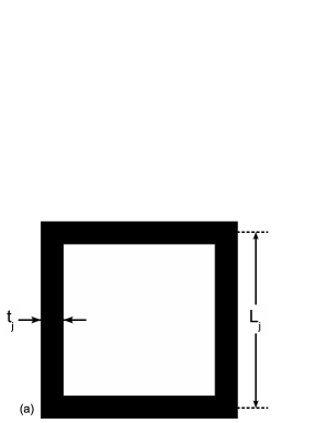
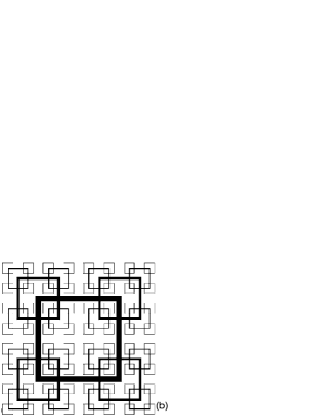
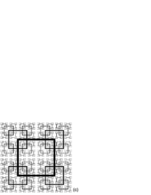
Figure 1: (a) Space-filling multiscale/fractal square grid generating pattern. Examples of planar multiscale/fractal square grids used in the present work with N=4 scales (b) and N=5 scales (c).

A total of four different planar space-filling fractal square grids have been used in the wind tunnel experiments reported here. The complete planar geometry of these grids is detailed in table 1. Scaled-down diagrams of two of these grids are displayed in figures 1 and 1. Multiscale/fractal grids are clearly designed to generate turbulence by directly exciting a wide range of fluctuation length-scales in the flow rather than by relying on the non-linear cascade mechanism for multiscale excitation. The latter approach is the classical one and is exemplified by the use of regular grids as homogeneous turbulence generators.

Grid	SFG8	SFG13	SFG17	BFG17
$L_{0}(mm)$	237.5	237.7	237.8	471.2
$L_{1}(mm)$	118.8	118.9	118.9	235.6
$L_{2}(mm)$	59.4	59.4	59.5	117.8
$L_{3}(mm)$	29.7	29.7	29.7	58.9
$L_{4}(mm)$	-	-	-	29.5
$t_{0}(mm)$	14.2	17.2	19.2	23.8
$t_{1}(mm)$	6.9	7.3	7.5	11.7
$t_{2}(mm)$	3.4	3.1	2.9	5.8
$t_{3}(mm)$	1.7	1.3	1.1	2.8
$t_{4}(mm)$	-	-	-	1.4

Table 1: Geometry of the space-filling fractal square grids.

As explained in [15], the complete design of space-filling grids requires a total of four independent parameters such as :

• $N$ : the number of scales ($N-1$ being the number of scale-iterations),

• $L_{0}$ : the biggest bar length of the grid

• $t_{0}$ : the biggest bar thickness of the grid

• $t_{N-1}$ : the smallest bar thickness of the grid

The smallest bar length $L_{N-1}$ on the grid is determined by $R_{L}=1/2$ and $N$. Note, also, that the fractal grids are manufactured from an acrylic plate with a constant thickness ($5mm$) in the direction of the mean flow.

Hurst & Vassilicos [15] introduced the thickness ratio $t_{r}=\frac{t_{0}}{t_{N-1}}$ and the effective mesh size

$$M_{eff}=\frac{4T^{2}}{P}\sqrt{1-\sigma}$$ (1)

where $P$ is the fractal perimeter length of the grid, $T^{2}$ is the tunnel’s square cross section and $\sigma$ is the blockage ratio of the grid defined as the ratio of the area $A$ covered by the grid to $T^{2}$:

$$\sigma=\frac{A}{T^{2}}=\frac{L_{0}t_{0}\sum_{j=0}^{N-1}4^{j+1}R_{L}^{j}R_{t}^{j}-t_{0}^{2}\sum_{j=1}^{N-1}2^{2j+1}R_{t}^{2j-1}}{T^{2}}.$$ (2)

These quantities are derivable from the few independent geometrical parameters chosen to uniquely define the grids. When applied to a regular grid, this definition of $M_{eff}$ returns its mesh size. When applied to a multiscale grid where bar sizes and local blockage are inhomogeneously distributed across the grids, it returns an average mesh size which was shown in [15] to be fluid mechanically relevant.

A total of four space-filling fractal square grids have been used in the present work. They all have the same blockage ratio $\sigma=0.25$ (low compared to regular grids where, typically, $\sigma$ is about 0.35 or 0.4 or so [8], [7]) and turn out to have values of $M_{eff}$ which are all very close to $26.4mm$. Three of these grids, refered to as SFG8, SFG13 and SFG17, differ by only one parameter, $t_{r}$, and as a consequence also by the values of $t_{j}$ ($0\leq j\leq N-1$) as $t_{r}$ was chosen to be one of the four all-defining parameters along with the fixed parameters $N=4$, $L_{3}=29.7mm$ and $\sigma=0.25$. The fourth grid, BFG17, has one extra iteration, i.e. $N=5$ instead of $N=4$ but effectively the same smallest length, i.e. $L_{4}=29.5mm$, and a value of $t_{r}$ very close to that of SFG17. It is effectively very similar to SFG17 but with one extra fractal iteration. The main characteristics of these grids are summarized in tables 1 and 2 which also includes values for $L_{r}\equiv L_{0}/L_{N-1}$.

Grid	$N$	$L_{0}(mm)$	$t_{0}(mm)$	$L_{r}$	$t_{r}$	$\sigma$	$M_{eff}(mm)$
SFG8	4	237.5	14.2	8	8.5	0.25	26.4
SFG13	4	237.7	17.2	8	13.0	0.25	26.3
SFG17	4	237.8	19.2	8	17.0	0.25	26.2
BFG17	5	471.2	23.8	16	17.0	0.25	26.6

Table 2: Main characteristics of the fractal square grids.

In addition to the fractal grids, we have also performed a comparative study of turbulence generated by a regular grid, refered as SRG hereafter, made of a bi-plane square rod array. Table 3 presents the main properties of this grid. Its blockage ratio is higher than that of our fractal grids and closer to the usual values found in literature for regular grids (see e.g. [2], [8]). The regular grid SRG also has slightly higher mesh size.

Grid	$N$	$L_{0}(mm)$	$t_{0}(mm)$	$L_{r}$	$t_{r}$	$\sigma$	$M_{eff}(mm)$
SRG	4	460	6	8	1	0.34	32

Table 3: Main characteristics of the regular grid.

3 The experimental set-up

3.1 The wind tunnels

Measurements are performed in two air wind tunnels, one which is open-circuit with a $5m$ long and $T=0.46m$ wide square test section and one which is recirculating with a $5.4m$ long and $T=0.91m$ wide square test section. A generic sketch of a tunnel’s square test section is given in figure 2 for the purpose of defining spatial coordinate notation. The arrow in this figure indicates the direction of the mean flow and of the inlet velocity $U_{\infty}$. The turbulence-generating grids are placed at the inlet of the test section.

The fractal grids SFG8, SFG13, SFG17 and the regular grid SRG were tested in the open circuit tunnel whereas the fractal grid BFG17 was tested in the recirculating tunnel.

The maximum flow velocity without a grid or any other obstruction is $33m/s$ in the $T=0.46m$ open-circuit tunnel. Turbulence-generating grids were tested with three values of the inlet velocity $U_{\infty}$ in this tunnel: $5.2m/s$, $10m/s$ and $15m/s$. The uniformity of the inlet velocity at the convergent’s outlet, checked with Pitot tube measurements, is better than 5%. The residual turbulence intensity in the absence of a turbulent-generating grid is about 0.4% along the axis of the tunnel.

In the $T=0.91m$ recirculating tunnel, the maximum flow velocity without a grid or any other obstruction is $45m/s$. The inlet velocity $U_{\infty}$ was fixed at $5.2m/s$ in this facility when testing the turbulence generated by the BFG17 grid. The entrance flow uniformity is better than 2% and a very low residual turbulence intensity ($\leq 0.05$%) remains in the test section in the absence of a turbulence-generating grid or obstacle.

In both tunnels, the temperature is monitored during measurement campaigns thanks to a thermometer sensor located at the end of the test section. The inlet velocity $U_{\infty}$ is imposed by measuring the pressure difference in the tunnel’s contractions with a micromanometer Furness Controls MCD1001.

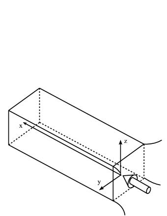
Figure 2: Wind-tunnel sketch and coordinate notation

3.2 Velocity measurements

A single hot-wire, running in constant-temperature mode, was used to measure the longitudinal velocity component. The DANTEC 55P01 single probe was driven by a DISA 55M10 anemometer and the probe was mounted on an aluminum frame allowing 3D displacements in space. A systematic calibration of the probe was performed at the beginning and at the end of each measurement campaign and the temperature was monitored for thermal compensation. The sensing part of the wire (PT-0.1Rd) was $5\mu m$ in diameter ($d_{w}$) and about $1mm$ in length $l_{w}$ so that the aspect ratio $\frac{l_{w}}{d_{w}}$ was about $200$. Our spatial resolution $l_{w}/\eta$ ranges between $2$ and $9$ for all the measurements. The estimated frequency response of this anemometry system is $1.5$ to $9$ times higher than the Kolmogorov frequency $f_{\eta}=\frac{U}{2\pi\eta}$. The spatially-varying longitudinal velocity component $\tilde{u}(x)$ in the direction of the mean flow was recovered from the time-varying velocity $\tilde{u}(t)$ measured with the hot-wire probe by means of local Taylor’s hypothesis as defined in [16].

The signal coming from the anemometer was compensated and amplified with a DISA 55D26 signal conditioner to enhance the signal to noise ratio which is typically of the order of $45dB$ for all measurements. The uncertainties on the estimation of the dissipation rate $\epsilon$ due to electronic noise occurring at high frequencies (wavenumbers) is lower than 4% for all our measurements. The conditioned signal was low-pass filtered to avoid aliasing and then sampled by a 16 bits National Instruments NI9215 USB card. The sampling frequency was adjusted to be slightly higher than twice the cut-off frequency. The sampled signal was then stored on the hard-drive of a PC. The signal acquisition was controlled with the commercial software LabVIEW©, while the post-processing was carried out with the commercial software MATLAB©.

The range of Reynolds numbers and lengths-scales of the turbulent flows generated in both tunnels by all our grids are summarized in table 4. The longitudinal integral length-scale $L_{u}$ was obtained by integrating the autocorrelation function of the fluctuating velocity component $u(x)$ (obtained by subtracting the average value of $\tilde{u}(x)$ from $\tilde{u}(x)$):

$$L_{u}=\int_{0}^{\infty}\frac{\left\langle u(x)u(x+\Delta)\right\rangle}{\left\langle u(x)^{2}\right\rangle}d\Delta$$ (3)

where the averages are taken over time, i.e. over $x$ in this equation’s notation, where $x$ is obtained from time $t$ by means of the local Taylor hypothesis. In this paper we use the notation $u^{\prime}\equiv\sqrt{\left\langle u(x)^{2}\right\rangle}$.

The Taylor microscale $\lambda$ was computed via the following expression:

$$\lambda=\sqrt{\frac{\left\langle u^{2}\right\rangle}{\left\langle\left(\partial u/\partial x\right)^{2}\right\rangle}}.$$ (4)

Finally, using the kinematic viscosity $\nu$ of the fluid (here air at ambient temperature) we also calculate the length-scale

$$\eta=\left(\frac{\nu^{2}}{15\left\langle\left(\partial u/\partial x\right)^{2}\right\rangle}\right)^{1/4}$$ (5)

which is often refered to as Kolmogorov microscale. We have estimated from the turbulent kinetic energy budget that the uncertainties in the computation of $\lambda$ and $\eta$ are lower than 10% and 5% respectively for all our measurements.

$T[m]$	$U_{\infty}[m/s]$	$L_{u}[mm]$	$\lambda[mm]$	$\eta[mm]$	$Re_{\lambda}$
$0.46$	$5/10/15$	$43-52$	$4-7.4$	$0.11-0.32$	$140-370$
$0.91$	$5$	$50-70$	$7-10$	$0.3-0.45$	$60-220$

Table 4: Main flow characteristics: $T$ is the wind tunnel width, $L_{u}$ is the longitudinal integral length-scale, $\lambda$ the Taylor-microscale, $\eta$ the Kolmogorov scale and $Re_{\lambda}$ the Taylor based Reynolds number.

4 Results

Hurst & Vassilicos [15] found that the streamwise and spanwise turbulence velocity fluctuations generated by the space-filling fractal square grids used here increase in intensity along $x$ on the centreline till they reach a point $x=x_{peak}$ beyond which they decay. Thus they defined the production region as being the region where $x<x_{peak}$ and the decay region as being the region where $x>x_{peak}$. They also found that various turbulence statistics collapse when plotted as functions of $x/x_{peak}$ and they attempted to give an empirical formula for $x_{peak}$ as a function of the geometric parameters of the fractal grid. It was also clear in their results that the turbulent intensities depend very sensitively on parameters of the fractal grids even at constant blockage ratio, thus generating much higher turbulence intensities than regular grids. An understanding and determination of how $x_{peak}$ and turbulence intensities depend on fractal grid geometry matters critically both for achieving a fundamental understanding of multiscale-generated turbulence and for potential applications such as in mixing and combustion. In such applications, it is advantageous to generate desired high levels of turbulence intensities at flexibly targeted downstream positions with as low blockage ratios and, consequently, pressure drop and power input, as possible. An important question left open, for example, in [15] is whether $x_{peak}$ does or does not depend on $U_{\infty}$.

This section is subdivided in eight subsections. In the first we study the steamwise profiles of the streamwise mean velocity and turbulence intensity and, in particular, determine $x_{peak}$. In the second we offer data which describe how homogeneity of mean flow and turbulence intensities is achieved when passing from the production to the decay region. In the third subsection we present results on the turbulent velocity skewness and flatness. The fourth and eightth subsections are a careful application of the theory of George & Wang [12] to our data and the fifth, sixth and seventh subsections are an investigation of the single-length scale assumption of this theory and its consequences, in particular the extraordinary property first reported in [31] that the ratio of the integral to the Taylor length-scales is independent of $Re_{\lambda}\equiv{u^{\prime}\lambda/\nu}$ in the fractal-generated homogeneous decaying turbulence beyond $x_{peak}$.

4.1 The wake-interaction length-scale $x_{\star}$

The dimensionless centreline mean velocity $U_{C}/U_{\infty}$ and the centreline turbulence intensity $u^{\prime}_{c}/U_{C}$ are plotted in figures 3 and 3 for all space-filling fractal square grids as well as for the regular grid SRG. For the latter, we have fitted the turbulence intensity $u^{\prime}_{c}/U_{C}$ with the well-known power-law $A\left(\frac{x-x_{0}}{M_{eff}}\right)^{-n}$ where the dimensional parameter $A$, the exponent $n$ and the virtual origin $x_{0}$ have been empirically determined following the procedure introduced by Mohamed & LaRue [26]. Our results are in excellent agreement with similar results reported in the literature for regular grids, e.g. $n=1.41$ is very close to the usually reported empirical exponent (see [26] and references therein).

Figure 3 confirms that a protracted production region exists in the lee of space-filling fractal square grids, that it extends over a distance which depends on the thickness ratio $t_{r}$ and that it is followed by a region (the decay region first identified in [15]) where the turbulence decays. The existence of a distance $x_{peak}$ where the turbulence intensity peaks is clear in this figure. Figure 3 shows that the production region where the turbulence increases is accompanied by significant longitudinal mean velocity gradients which progressively decrease in amplitude till about after $x=x_{peak}$ where they more or less vanish and the turbulence intensity decays.

Our data show that the centreline mean velocity is quite high compared to $U_{\infty}$ on the close downstream side of our fractal square grids and remains so over a distance which depends on fractal grid geometry before decreasing towards $U_{\infty}$ further downstream. This centreline jet-like behavior seems to result from the relatively high opening at the grid’s centre where blockage ratio, which is inhomogeneously distributed on the grid, seems to be locally small compared to the rest of the grid. The initial plateau is therefore characterized by a significant velocity excess ($U_{C}/U_{\infty}>1.35$). One can also see in figure 3 that the mean velocity remains larger than $U_{\infty}$ even far away from the grids. We have checked that this effect is consistent with the small downstream growth of the boundary layer on the tunnel’s walls.

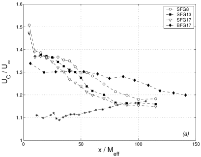
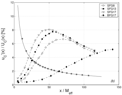
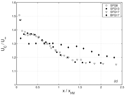
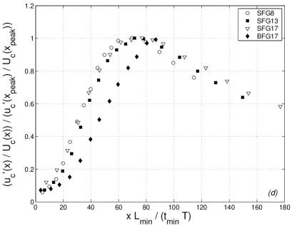
Figure 3: Streamwise evolution of (a) the centreline mean velocity $U_{C}/U_{\infty}$ and of (b) the turbulence intensity $u^{\prime}_{c}/U_{C}$ for all fractal grids with respect to the streamwise distance $x$ scaled by $M_{eff}$. Streamwise evolution of (c) the centreline mean velocity $U_{C}/U_{\infty}$ and of (d) the turbulence intensity $u^{\prime}_{c}/U_{C}$ normalised by its value at $x=x_{peak}$ for all fractal grids with respect to the streamwise distance $x$ scaled by $x_{HV}=75t_{min}T/L_{min}$ [15] ($U_{\infty}=5.2m/s$). For reference, data obtained with the regular grid SRG and $U_{\infty}=10m/s$, are also reported ($\ast$ symbols in (b)). The power law $(u^{\prime}_{c}/U_{C})^{2}=A\left(\frac{x-x_{0}}{M_{eff}}\right)^{-1.41}$ which is also shown (solid line in (b), $A=0.129$, $x_{0}=0$) fits this SRG data very well.

The space-filling fractal grids SFG8, SFG13 and SFG17 are identical in all but one parameter: the thickness ratio $t_{r}$. It is therefore clear from figures 3 and 3 that $t_{r}$ plays an important role because, even though the streamwise profiles of $U_{C}/U_{\infty}$ and $u^{\prime}_{c}/U_{C}$ are of identical shape for SFG8, SFG13 and SFG17, $U_{C}/U_{\infty}$ decreases, $u^{\prime}_{c}/U_{C}$ increases and $x_{peak}$ decreases when increasing $t_{r}$ whilst keeping all other independent parameters of the grid constant.

However, the parameter $t_{r}$ cannot account alone for the differences between the SFG17 and BFG17 grids. These two grids have the same blockage ratio $\sigma$ and very close values of $t_{r}$ and effective mesh size $M_{eff}$. What they do mainly differ by, are their values of $L_{0}$ (by a factor of 2), the number of fractal iterations ($N=4$ for SFG17, $N=5$ for BFG17) and the largest thickness $t_{0}$. Figures 3 and 3 show clearly that when $t_{r}$ is kept roughly constant and other grid parameters are varied (such as $L_{0}$), then $x_{peak}$ and the overall streamwise profiles of $U_{C}/U_{\infty}$ and of $u^{\prime}_{c}/U_{C}$ change in ways not accounted for by the changes between SFG8,SFG13 and SFG17.

Comparing data obtained downstream from different space-filling fractal square grids, Hurst & Vassilicos [15] suggested that the streamwise evolution of turbulence intensity, i.e. $x_{peak}$, can be scaled by the length-scale $x_{HV}=75\frac{t_{min}T}{L_{min}}$. Their empirical formula might appear to account for the difference between the SFG17 and BFG17 grids in figure 3(b) because $T$ is double and $t_{min}$ is larger by a factor 1.3 for BFG17 compared to SFG17. However, Hurst & Vassilicos [15] did not attempt to collapse data from different wind tunnels, and we now show how such a careful collapse exercise involving both the mean flow and the turbulence intensity leads to a different formula for $x_{peak}$.

In figures 3 and 3 we plot the streamwise evolution of $U_{C}/U_{\infty}$ and of $u^{\prime}_{c}/U_{C}$ (scaled by its value at $x_{peak}$) using the scaling $x/x_{HV}$ introduced by Hurst & Vassilicos [15]. One can clearly see that whilst use of $x_{HV}$ collapses the data obtained in the T=0.46m tunnel, a large discrepancy remains with the T=0.91m tunnel data. In particular, $x_{peak}$ differs for BFG17 and SFG17.

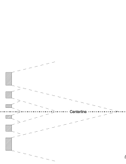
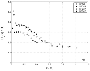
Figure 4: (a) Schematic of wake interactions resulting from the fractal grid’s bars. (b) Centreline mean streamwise velocity vs distance normalised by the wake-interaction length scale $x_{*}=L_{0}^{2}/t_{0}$ ($U_{\infty}=5.2m/s$).

The turbulence generated by either regular or multiscale/fractal grids with relatively low blockage ratio results from the interactions between the wakes of the different bars. In the case of fractal grids these bars have different sizes and, as a result, their wakes interact at different distances from the grid according to size and position on the grid (see direct numerical simulations of turbulence generated by fractal grids in [28], [19] and [18]). Assuming that the typical wake-width $\ell$ at a streamwise distance $x$ from a wake-generating bar of width/thickness $t_{j}$ ($j=0,...,N-1$) to be $\ell\sim\sqrt{t_{j}x}$ [37], the largest such width corresponds to the largest bars on the grid, i.e. $\ell\sim\sqrt{t_{0}x}$. Assuming also that this formula can be used even though the bars are surrounded by other bars of different sizes, then the furthermost interaction between wakes will be that of the wakes generated by the largest bars placed furthermost on the grid (see figure 4). This will happen at a streamwise distance $x=x_{\star}$ such that $L_{0}\sim\ell\sim\sqrt{t_{0}x_{\star}}$. We therefore introduce

$$x_{\star}=\frac{L_{0}^{2}}{t_{0}}$$ (6)

as a characteristic length-scale of interactions between the wakes of the grid’s bars which might bound $x_{peak}$. We stress that the assumptions used to define $x_{\star}$ are quite strong and care should be taken in extrapolating this presumed bound on $x_{peak}$ to any space-filling fractal square grid beyond those studied here, let alone any fractal/multiscale grid.

Figure 4 is a plot of the normalised centreline mean velocity $U_{C}/U_{\infty}$ as a function of dimensionless distance $x/x_{\star}$ for all our four space-filling fractal square grids. All the data from the T-0.46m tunnel collapse in this representation. However the BFG17 data from the larger wind tunnel do not. They fall on a similar curve but at lower values of $U_{C}/U_{\infty}$. This systematic difference can be explained by the fact that the air flow causes the BFG17 grid in the large wind tunnel to bulge out a bit and adopt a slightly curved but steady shape. The flow rate distribution through this grid must be slightly modified as a result. To compensate for this effect we introduce the mean velocity $U_{p}$ characterizing the constant mean velocity plateau in the vicinity of the fractal grids. In figure 5 we plot the normalised centreline mean velocity $U_{C}/U_{p}$ as a function of $x/x_{\star}$ for all fractal grids and both tunnels and find an excellent collapse onto a single curve.

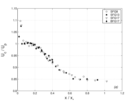
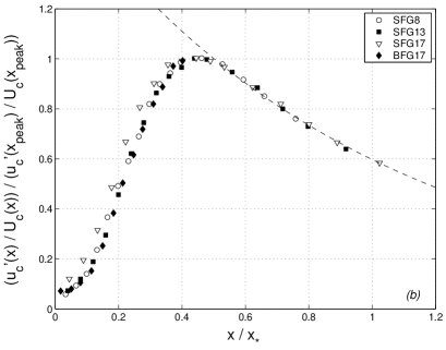
Figure 5: Streamwise evolution of (a) the centreline mean velocity $U_{C}$ normalized by the initial mean velocity plateau $U_{p}$ and (b) centreline turbulence intensity normalised by its value at $x=x_{peak}$. Both plots are given as functions of $x$ scaled by the wake-interation length-scale $x_{\star}=L_{0}^{2}/t_{0}$ ($U_{\infty}=5.2m/s$). In (b) the dashed line represents equation (9) with $B=2.06$ and $A=2.82$.

In figure 5 we plot $u^{\prime}_{c}/U_{C}$ normalised by its value at $x_{peak}$ as a function of $x/x_{\star}$. We also find an excellent collapse onto a single curve irrespective of fractal grid and tunnel. It is also clear from figures 5 and 5 that the longitudinal mean velocity gradient $\frac{\partial U}{\partial x}$ becomes insignificant where $x\geq 0.6x_{\star}$ and that the streamwise turbulence intensity peaks at

$$x_{peak}\approx 0.45x_{\star}=0.45\frac{L_{0}^{2}}{t_{0}}.$$ (7)

The wake-interaction length-scale $x_{\star}$ appears to be the appropriate length-scale characterising the first and second order statistics of turbulent flows generated by space-filling fractal square grids, at least on the centreline and for the range of grids tested in the present work.

In figures 6 and 6 we plot the streamwise evolutions of the dimensionless centreline velocity $U_{C}/U_{\infty}$ and the centreline turbulence intensity $u^{\prime}_{c}/U_{C}$ for various inlet velocities $U_{\infty}$. These particular results have been obtained for the fractal grid SFG17 but they are representative of all our space-filling fractal square grids. One can clearly see that $x_{peak}$ is independent of $U_{\infty}$. Moreover, our data show that the entire streamwise profiles of both $U_{C}/U_{\infty}$ and $u^{\prime}_{c}/U_{C}$ are also independent of the inlet velocity $U_{\infty}$ in the range studied.

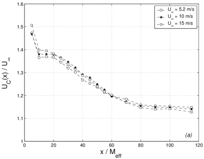
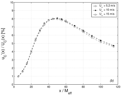
Figure 6: (a) Streamwise evolution of the centreline ($y=z=0$) mean velocity in the T-0.46 tunnel for the fractal grid SFG17. (b) Streamwise evolution of the turbulence intensity for the same grid and in the same tunnel.

Hurst & Vassilicos [15] have shown that the centreline turbulence intensity decays exponentially in the decay region $x>x_{peak}$ and that the length-scale $x_{peak}$ can be used to collapse this decay for different space-filling fractal square grids as follows:

$${\frac{u^{\prime 2}_{c}}{U_{C}^{2}}}={u^{\prime 2}_{c}(x_{0})\over U_{C}^{2}(x_{0})}exp\left(-B^{\prime}\left(\frac{x-x_{0}}{x_{peak}}\right)\right)$$ (8)

where $x_{0}$ is a virtual origin and $B^{\prime}$ an empirical dimensionless parameter. We confirm this scaling decay form, specifically by fitting

$${u^{\prime 2}_{c}\over U_{C}^{2}}=Aexp\left(-B\left(\frac{x}{x_{*}}\right)\right)$$ (9)

to our experimental data with a slightly modified dimensional parameter $B$ and an extra dimensionless parameter $A$ which does not have much influence on the quality of the fit except for shifting it all up or down. We have arbitrarily set $x_{0}=0$, which we are allowed to do because the virtual origin does not affect the value of $B$. It only affects the value of $A$.

As shown in figure 5 the exponential decay law (9) is in excellent agreement with our data for all the space-filling fractal square grids used in the present work. In particular, the parameter $B$ seems to be the same for all the fractal square grids we used. Using a least-mean square method we find $B=2.06$ and $A=2.82$.

Evidence in support of the idea that the decay region around the centreline downstream of $x_{peak}$ is approximately homogeneous and isotropic was given in [31]. The exponential turbulence decay observed in this region ([15], [31]) is therefore remarkable because it differs from the usual power-law decay of homogeneous isotropic turbulence. We have already reported in this subsection that the mean flow becomes approximately homogeneous in the streamwise direction where $x>0.6x_{\star}$, i.e. in the decay region. In the following subsection we investigate the spanwise mean flow and turbulence fluctuation profiles downstream from space-filling fractal square grids and show how a highly inhomogeneous flow near the fractal grid morphs into a homogeneous one beyond $0.6x_{\star}$.

4.2 Homogeneity

Like regular grids, the flow generated in the lee of space-filling fractal square grids is marked by strong inhomogeneities near the grid which smooth out further downstream under the action of turbulent diffusion. This is evidenced in figures 7 and 7 which show scaled mean velocity $U/U_{c}$ and turbulence intensity $u^{\prime}/U$ profiles along the diagonal in the $y-z$ plane, i.e. along the line parameterised by $(y^{2}+z^{2})^{1/2}$ in that plane. Close to the grid, the mean velocity profile is very irregular, especially downstream from the grid’s bars where large mean velocity deficits are clearly present. These deficits are surrounded by high mean flow gradients where the intense turbulence levels reach local maxima as shown in figure 7. Further downstream, both mean velocity and turbulence intensity profiles become much smoother supporting the view that the turbulence tends towards statistical homogeneity. Note that figures 7 and 7 show diagonal profiles at $x/M_{eff}\approx$ $7$ and $53$ in the lee of the BFG17 grid which is a long way before $x_{peak}$ (see figure 3b). The profiles are quite uniform in the decay region as shown by Seoud & Vassilicos [31]. Our evidence for homogeneity complements theirs in two ways: they concentrated only on the decay region whereas we report profiles in the production region and how they smooth out along the downstream direction; and we report diagonal profiles whereas the profiles in [31] are all along the $y$ coordinate.

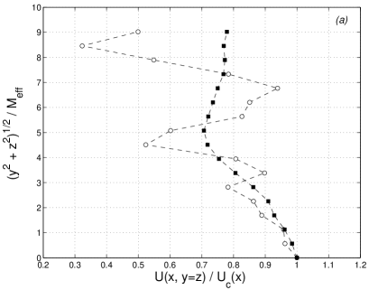
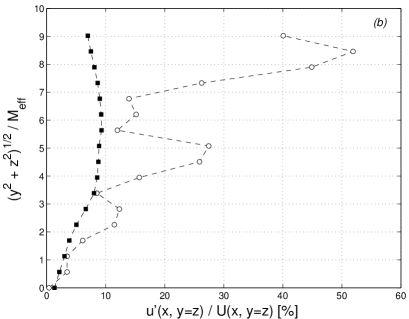
Figure 7: (a) Normalised mean velocity profiles and (b) turbulence intensity profiles along the diagonal line in the T-0.91m tunnel. The fractal grid is BFG17. Symbols: $\bigcirc$, $x/M_{eff}\approx 7$ (i.e. $x/x_{*}\approx 0.02$); $\blacksquare$, $x/M_{eff}\approx 53$ (i.e. $x/x_{*}\approx 0.15$).

To evaluate the distance from the grid where the inlet inhomogeneities become negligible, we introduce the ratios $U_{c}/U_{d}$ and $u^{\prime}_{c}/u^{\prime}_{d}$ where subscripts $c$ and $d$ denote respectively the centreline ($y=z=0$) and the streamwise line cutting through the second iteration corner ($y=z=6cm$ in the SFG17 case) as shown in figure 8. These two straight lines meet the inlet conditions at two different points, their difference being representative of the actual inhomogeneity on the fractal grid itself: one point is at the central empty space whilst the other is at the corner of one of the second iteration squares. The streamwise evolutions of $U_{c}/U_{d}$ and $u^{\prime}_{c}/u^{\prime}_{d}$ are reported in figure 8. As expected, large differences are observable in the vicinity of the space-filling fractal square grid for both the mean and the fluctuating velocities. One can see that the mean velocity ratio $U_{c}/U_{d}$ is bigger than unity. This reflects the mean velocity excess on the centreline where the behaviour is jet-like because of the local opening compared to the mean velocity deficit downstream from the second iteration corner where the behaviour is wake-like because of the local blockage. This difference between jet-like and wake-like local behaviours also explains why the fluctuating velocity ratio $u^{\prime}_{c}/u^{\prime}_{d}$ is almost null close to the grid where the centreline is almost turbulence free. Further downstream, both ratios $U_{c}/U_{d}$ and $u^{\prime}_{c}/u^{\prime}_{d}$ tend to unity as the flow homogenises. One can see that inhomogeneities become negligible by these criteria beyond $x/x_{\star}=0.6$, which is quite close to $x_{peak}$.

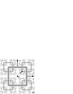
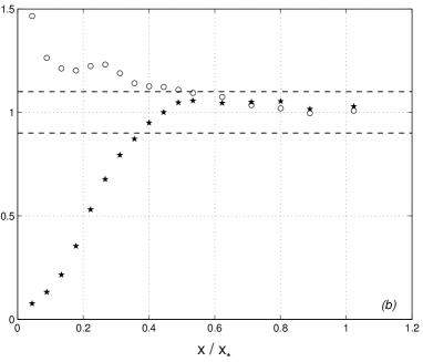
Figure 8: (a) The measurements in (b) are taken in the T-0.46m tunnel along the straight lines which run in the $x$-direction and cut the plane of the pictured SFG17 grid at points $c$ and $d$. (b) Streamwise evolution of the ratios $U_{c}/U_{d}$ ($\circ$) and $u^{\prime}_{c}/u^{\prime}_{d}$ ($\star$) measured for the SFG17 grid in the T-0.46m tunnel ($U_{\infty}=5.2m/s$). The horizontal dashed lines represent the range $\pm 10$%.

A main consequence of statistical homogeneity is that the small-scale turbulence is not sensitive to mean flow gradients. For this to be the case, the time scales defined by the mean flow gradients must be much larger than the largest time-scale of the small-scale turbulence. From our measurements and those in [31] (see figure 3 in [31]), $(\partial U/\partial x)^{-1}$ and $(\partial U/\partial y)^{-1}$ are always larger than about 1 and 0.15 second, respectively, at and beyond $x_{peak}$ where the time-scale of the energy-containing eddies is well below 0.07 seconds. The ratios between the smallest possible estimate of a mean shear time scale and any turbulence fluctuation time scale are therefore well above 2 (in the worst of cases) at $x_{peak}$ and far larger (by one or two orders of magnitude typically) beyond it for all three fractal grids SFG8, SFG13 and SFG17 and all inlet velocities $U_{\infty}$ in the range tested. By this time-scale criterion, from $x_{peak}$ onwards, the small-scale turbulence generated by our fractal grids, including the energy-containing eddies, is not affected by the typically small mean flow gradients which are therefore negligible in that sense.

We close this subsection with figure 9 which illustrates in yet another way the homogeneity of the turbulence intensity at $x\geq 0.5x_{*}$ and suggests that equation (9) can be extended beyond the centreline in the $y-z$ plane in that homogeneous region $x\geq 0.5x_{*}$, i.e.

$${u^{\prime 2}\over U^{2}}=Aexp\left(-B\left(\frac{x}{x_{*}}\right)\right)$$ (10)

with the same values $A\approx 2.82$ and $B\approx 2.06$ independently of $U_{\infty}$ and space-filling fractal square grid. It is worth pointing out, however, that figure 9 also shows quite clearly that $x_{peak}$ can vary widely across the $y-z$ plane and that a very protracted production region does not exist everywhere. Formula (7) gives $x_{peak}$ on the centreline but $x_{peak}$ can be very much smaller than $0.45x_{*}$ at other $y-z$ locations. This is a natural consequence of the inhomogeneous blockage of fractal grids and the resulting combination of wake-like and jet-like regions in the flows they generate.

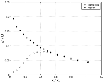
Figure 9: Streamwise turbulence intensities as functions of $x/x_{*}$ along the centreline and along the straight streamwise line which crosses point $d$ in Fig. 8(a). SFG17 grid in the T-0.46m tunnel with $U_{\infty}=15m/s$. This plot remains essentially the same for the other values of $U_{\infty}$ that we tried.

4.3 Skewness and flatness of the velocity fluctuations

Previous wind tunnel investigations of turbulence generated by space-filling fractal square grids [15], [31] have not reported results on the gaussianity/non-gaussianity of turbulent velocity fluctuations. We therefore study here this important aspect of the flow, mostly in terms of the skewness $S_{u}=\frac{\left\langle u^{3}\right\rangle}{\left\langle u^{2}\right\rangle^{3/2}}$ and flatness $F_{u}=\frac{\left\langle u^{4}\right\rangle}{\left\langle u^{2}\right\rangle^{2}}$ of the longitudinal fluctuating velocity component $u$ along the centreline. This skewness is also a measure of one limited aspect of large-scale isotropy, namely mirror symmetry, as it vanishes when statistics are invariant to the transformation $u$ to $-u$, but not otherwise. Isotropy was studied in much more detail in [15] and [31] where x-wires were used. These previous works reported good small-scale isotropy in the decay region [31] and levels of large-scale anisotropy before and after $x_{peak}$ on the centreline [15] which, for the turbulence generated by the grids SFG13, SFG17 and BFG17 in particular, are very similar to the levels of large-scale anisotropy in turbulence generated by active grids [22], [27].

We first check that both $S_{u}$ and $F_{u}$ do not depend on the inlet velocity $U_{\infty}$, and this is indeed the case as shown in figures 10(a) and 10(b). These plots are particularly interesting in that they reveal the existence of large values of both $S_{u}$ and $F_{u}$ at about the same distance from the grid on the centreline. This distance scales with the wake-interaction length-scale $x_{*}$ as shown in figures 11 and 12. Indeed, the profiles of both $S_{u}$ and $F_{u}$ along the centreline collapse for all four fractal square grids (SFG8, SFG13 and SFG17 in the T-0.46m tunnel and BFG17 in the T-0.91m tunnel) when plotted against $x/x_{*}$. The alternative plots against $x/M_{eff}$ clearly do not collapse (see figures 11(a) and 12(a)).

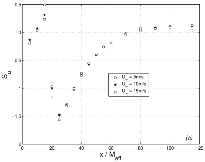
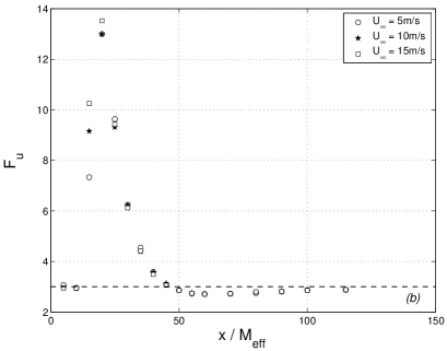
Figure 10: (a) Skewness and (b) flatness of the longitudinal fluctuating velocity component $u$ as functions of $x/M_{eff}$ along the centreline. SFG17 grid in the T-0.46m tunnel. The dashed lined in the right plot is $F_{u}=3$.

For comparison, figure 11(a) contains data of $S_{u}$ obtained with the regular grid SRG which are in fact in good agreement with usual values reported in the literature (see e.g. [3], [26]). It is well known that regular grids generate small, yet non-zero, positive values of the velocity skewness $S_{u}$ and Maxey [24] explained how their non-vanishing values are in fact a consequence of the free decay of homogeneous isotropic turbulence. Whilst the velocity skewness $S_{u}$ generated by fractal grids takes values which are also close to zero yet clearly positive in the decay region, $S_{u}$ behaves very differently in the production region on the centreline.

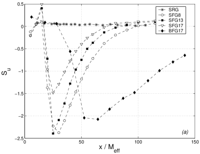
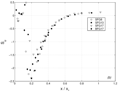
Figure 11: Velocity skewness $S_{u}$ as function of (a) $x/M_{eff}$ and (b) $x/x_{*}$. $U_{\infty}=5.2m/s$. Data corresponding to all fractal grids and to the regular grid SRG as per insert.

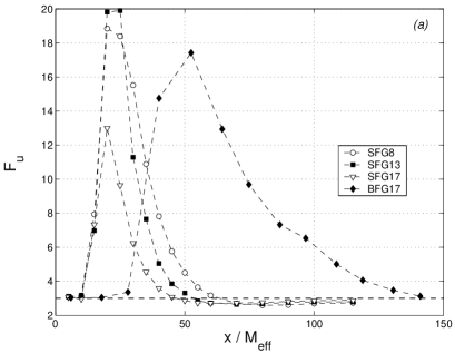
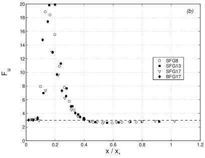
Figure 12: Velocity flatness $F_{u}$ as function of (a) $x/M_{eff}$ and (b) $x/x_{*}$. $U_{\infty}=5.2m/s$. Data corresponding to all fractal grids as per insert. The dashed line in both plots is $F_{u}=3$.

The behaviours of $S_{u}$ and $F_{u}$ in the production region on the centreline are both highly unusual as can be seen in figures 10, 11 and 12. Clearly some very extreme/intense events occur at $x\approx 0.2x_{*}$ and it is noteworthy that the location of these extreme events scales with $x_{*}$ even though it is clearly different from $x_{peak}\approx 0.45x_{*}$. The scatter observed at and around this location is due to lack of convergence because these intense events are quite rare as clearly seen in time traces such as the one given in figure 13(a). These intense events are so high in magnitude ($\left|S_{u}\right|\sim 1$) that they cannot be attributed to experimental uncertainties. The negative signs of $S_{u}$ and of these intense events on the time traces demonstrate clearly that these extreme events correspond to locally decelerating flow. We leave their detailed analysis for future study.

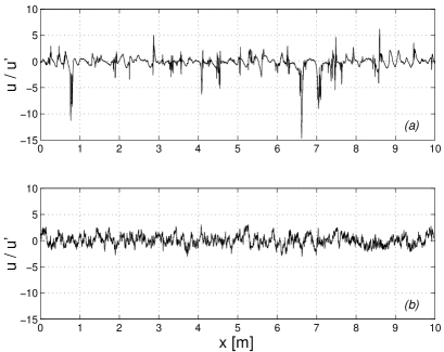
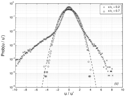
Figure 13: (a) and (b) Normalised velocity samples recorded downstream of the SFG17 fractal grid at (a) $x\approx 0.2x_{*}$ and (b)$x\approx 0.7x_{*}$. (c) Probability Density Function (PDF) computed from signals corresponding to the SFG17 grid such as those shown on the left. The dashed line is the Gaussian distribution. $U_{\infty}=5.2m/s$ for all the plots on this figure.

These extreme decelerating flow events are also reflected in the Probability Density Function (PDF) of u which is clearly non-gaussian and skewed to the left (i.e. towards negative $u$-values) at $x=0.2x_{*}$ whereas it is very closely gaussian in the decay region (see figure 13(b)). The flatness $F_{u}$ takes values close to the usual gaussian value of 3 in the decay region and remains close to 3 for all $x\geq x_{peak}$ (see figures 10(b) and 12(b)).

Note, finally, that (10) and $F_{u}\approx 3$ in the homogeneous region $x\geq 0.5x_{*}$ imply that

$${<u^{4}>\over U^{4}}\approx 3A^{2}exp\left(-2B\left(\frac{x}{x_{*}}\right)\right)$$ (11)

in that region, with the same values $A\approx 2.82$ and $B\approx 2.06$ independently of $U_{\infty}$ and space-filling fractal square grid.

4.4 Spectral energy budget in the decay region

In the region beyond $x_{peak}$ where the turbulence is approximately homogeneous and isotropic, the energy spectrum has been reported in previous studies [31], [15] to be broad with a clear power-law shaped intermediate range where the power-law exponent is not too far from -5/3. For this region we can follow George & Wang [12] who found a solution of the spectral energy equation

$${\partial\over\partial t}E(k,t)=T(k,t)-2\nu k^{2}E(k,t)$$ (12)

that implies an exponential rather than power-law turbulence decay. In this spectral energy equation, $E(k,t)$ is the energy spectrum and $T(k,t)$ is the spectral energy transfer at time $t$. The energy spectrum, if integrated, gives ${3\over 2}u^{\prime 2}$, i.e.

$${3\over 2}u^{\prime 2}=\int_{0}^{\infty}E(k,t)dk.$$ (13)

The correspondence between the time dependencies in these equations and the dependence on $x$ in our experiments is made via Taylor’s hypothesis.

George & Wang [12] showed that (12) admits solutions of the form

$$E(k,t)=E_{s}(t)f(kl(t),*)$$ (14)

$$T(k,t)=T_{s}(t)g(kl(t),*)$$ (15)

where the functions $f$ and $g$ are dimensionless, and that such solutions can yield an exponential turbulence decay. These solutions are single-length scale solutions (the length-scale $l(t)$) and therefore differ fundamentally from the usual Kolmogorov picture [9] which involves two different length scales, one outer and one inner, their ratio being an increasing function of Reynolds number. The argument $*$ in (14) and (15) represents any dependencies that there might be on boundary/inlet/initial conditions.

The exponential decay reported by George & Wang [12] exists provided that the length-scale $l(t)$ is independent of time, i.e. ${d\over dt}l=0$, and takes the form $u^{\prime 2}\sim\exp[-10\nu t/l^{2}]$. Unless $l^{2}\propto\nu$, this form does not obviously compare well with the exponential decay (10) because (10) is independent of Reynolds number. We now carefully apply the approach of George & Wang [12] to our data by making explicit use of all potential degrees of freedom and confirm that an exponential decay which perfectly fits (10) can indeed follow from their approach.

Consider

$$E(k,t)=E_{s}(t,U_{\infty},Re_{0},*)f(kl(t),Re_{0},*)$$ (16)

$$T(k,t)=T_{s}(t,U_{\infty},Re_{0},*)g(kl(t),Re_{0},*)$$ (17)

where $Re_{0}\equiv{U_{\infty}t_{0}\over\nu}$ is the Reynolds number which characterises the thickest bars on the fractal grid, $l(t)=l(t,Re_{0},*)$ and the argument $*$ includes various dimensionless ratios of bar lengths and bar thicknesses on the fractal grid, as appropriate. The functions $f$ and $g$ are again dimensionless. The conditions for (16) and (17) to solve (12) are (see [12] for the solution method)

$${d\over dt}E_{s}=-a{2\nu\over l^{2}}E_{s}$$ (18)

$$T_{s}=b{d\over dt}E_{s}$$ (19)

$${dl\over dt}/l=c{dE_{s}\over dt}/E_{s}$$ (20)

where $a$, $b$ and $c$ are dimensionless functions of $Re_{0}$ and $*$ (note that $a>0$). Under these solvability conditions, the spectral energy equation (12) collapses onto the dimensionless form

$$f(\kappa,Re_{0},*)+c(Re_{0},*)\kappa{d\over d\kappa}f(\kappa,Re_{0},*)=b(Re_{0},*)g(\kappa,Re_{0},*)+{\kappa^{2}f(\kappa,Re_{0},*)\over a(Re_{0},*)}$$ (21)

where $\kappa\equiv kl(t,Re_{0},*)$.

Two different families of solutions exist according to whether $c$ vanishes or not. If $c\not=0$, then $c$ must be negative and

$$l(t)=l(t_{0})[1+{4\nu a|c|\over l^{2}(t_{0})}(t-\tau_{0})]^{1/2}$$ (22)

$$E_{s}(t)=E_{s}(t_{0})[1+{4\nu a|c|\over l^{2}(t_{0})}(t-\tau_{0})]^{1/2c}$$ (23)

in terms of a virtual origin $\tau_{0}$. However, if $c=0$, then ${dl\over dt}=0$ and

$$E_{s}(t)\sim exp\left(-2a{\nu t\over l^{2}}\right).$$ (24)

It is this second set of solutions, the one corresponding to $c=0$, with which George & Wang [12] chose to explain the form (10).

From (24), (16) and (13) and making use of $t=x/U_{\infty}$ it follows that

$$u^{\prime 2}=u^{\prime 2}_{0}exp\left(-2a{\nu x\over l^{2}U_{\infty}}\right)$$ (25)

where $u^{\prime}_{0}=u^{\prime}_{0}(U_{\infty},Re_{0},*)$, $a=a(Re_{0},*)$ and $l(Re_{0},*)$ is independent of $x$. Our wind tunnel measurements in subsection 4.1 and those leading to (10) and its range of validity suggest that (24) and (10) are the same provided that $u^{\prime}_{0}/U_{\infty}$ is a dimensionless function of the geometric inlet parameters $*$ and nothing else, and that

$$a=1.03Re_{0}l^{2}(Re_{0},*)/L_{0}^{2}$$ (26)

if use is made of (6) and $B\approx 2.06$. In other words, the single-scale solution of George & Wang [12] fits our data provided that the single length-scale $l(Re_{0},*)$ is independent of $x$ (i.e. $c=0$), that the dimensionless coefficient $a$ in (18) depends on $Re_{0}$ and $*$ as per (26) and that $u^{\prime}_{0}$ scales with $U_{\infty}$. Under these conditions, it follows from equation (21) that the dimensionless spectral functions $f$ and $g$ satisfy

$$f(kl,Re_{0},*)=b(Re_{0},*)g(kl,Re_{0},*)+2Re_{0}^{-1}\left({L_{0}\over\sqrt{B}l(Re_{0},*)}\right)^{2}(kl)^{2}f(kl,Re_{0},*)$$ (27)

where $B\approx 2.06$. Integrating this dimensionless balance over $\kappa=kl$ yields

$$\int_{0}^{\infty}f(\kappa,Re_{0},*)d\kappa=2\left({L_{0}\over\sqrt{B}l(Re_{0},*)}\right)^{2}Re_{0}^{-1}\int_{0}^{\infty}\kappa^{2}f(\kappa,Re_{0},*)d\kappa$$ (28)

because the spectral energy transfer integrates to zero. This equality can be used in conjunction with (16), (13) and (6) to obtain a formula for the kinetic energy dissipation rate per unit mass, $\epsilon=2\nu\int_{0}^{\infty}k^{2}E(k,t)dk$:

$$\epsilon={3B\over 2}{u^{\prime 2}U_{\infty}\over x_{*}}\approx 3.1{u^{\prime 2}U_{\infty}\over x_{*}}.$$ (29)

This is an important reference formula which we have been able to reach by applying the George & Wang [12] theory and by confronting it with new measurements which we obtained for three different yet comparable fractal grids and three different inlet velocities $U_{\infty}$. These are the new measurements reported in subsections 4.1. and 4.2 and summarised by (10) and (6) along with the observation that $A$ and $B$ in (10) do not depend on $U_{\infty}$ and on the different parameters of the space-filling fractal square grids used.

4.5 Multiscale-generated single-length scale turbulence

No sufficiently well-documented boundary-free shear flow [34], [29] nor wind tunnel turbulence generated by either regular or active grids [26], [27] has turbulence properties comparable to those discussed here, namely an exponential turbulence decay (10), a dissipation rate $\epsilon$ proportional to $u^{\prime 2}$ rather than the usual $u^{\prime 3}$, and spectra which can be entirely collapsed with a single length-scale. It is therefore important to subject our data to further and more searching tests.

The downstream variation of the Reynolds number $Re\equiv{u^{\prime}L_{u}\over\nu}$ is different for different boundary-free shear flows. However, it is always a power-law of the normalised streamwise distance ${x-x_{0}\over L_{B}}$ where $L_{B}$ is a length characterising the inlet and $x_{0}$ is an effective/virtual origin. For example, $Re\sim({x-x_{0}\over L_{B}})^{-1/3}$ for axisymmetric wakes, $Re\sim({x-x_{0}\over L_{B}})^{0}$ for plane wakes and axisymmetric jets and $Re\sim({x-x_{0}\over L_{B}})^{1/2}$ for plane jets [34], [29]. The turbulence intensity’s downstream dependence on ${x-x_{0}\over L_{B}}$ is $\sim({x-x_{0}\over L_{B}})^{-2/3}$ for axisymmetric wakes, $\sim({x-x_{0}\over L_{B}})^{-1/2}$ for plane wakes and jets and $\sim({x-x_{0}\over L_{B}})^{-1}$ for axisymmetric jets [34], [29]. In wind tunnel turbulence generated by either regular or active grids the downstream turbulence also decays as a power law of ${x-x_{0}\over L_{B}}$ and so does $Re$ [26], [27]. In all these flows, as in fact in all well-documented boundary-free shear flows, the integral length scale $L_{u}$ and the Taylor microscale $\lambda$ grow with increasing $x$, and in fact do so as power laws of ${x-x_{0}\over L_{B}}$. Their ratio $L_{u}/\lambda$ is a function of ${x-x_{0}\over L_{B}}$ and of an inlet Reynolds number $Re_{0}\equiv{U_{\infty}L_{B}\over\nu}$ where $U_{\infty}$ is the appropriate inlet velocity scale. Estimating $\lambda$ from $\nu u^{\prime 2}/\lambda^{2}\sim\epsilon\sim u^{\prime 3}/L_{u}$ [1], [34], [29], it follows that $L_{u}/\lambda\sim Re_{0}^{1/2}({x-x_{0}\over L_{B}})^{-1/6}$ for axisymmetric wakes, $L_{u}/\lambda\sim Re_{0}^{1/2}({x-x_{0}\over L_{B}})^{0}$ for plane wakes and axisymmetric jets, $L_{u}/\lambda\sim Re_{0}^{1/2}({x-x_{0}\over L_{B}})^{1/4}$ for plane jets and $L_{u}/\lambda\sim Re_{0}^{1/2}({x-x_{0}\over L_{B}})^{-p}$ with $p>1/2$ for wind tunnel turbulence. These downstream dependencies on $Re_{0}$ and ${x-x_{0}\over L_{B}}$ can be collapsed together as follows:

$${L_{u}\over\lambda}\sim Re_{\lambda}$$ (30)

where $Re_{\lambda}\equiv{u^{\prime}\lambda\over\nu}$. This means that values of $L_{u}/\lambda$ obtained from measurements at different downstream locations $x$ but with the same inlet velocity $U_{\infty}$ and values of $L_{u}/\lambda$ obtained for different values of $U_{\infty}$ but the same downstream location fall on a single straight line in a plot of $L_{u}/\lambda$ versus $Re_{\lambda}$. This conclusion can in fact be reached for all sufficiently well-documented boundary-free shear flows [34] as for decaying homogeneous isotropic turbulence [29], [9] if the cornerstone assumption $\epsilon\sim u^{\prime 3}/L_{u}$ is used.

The relation $L_{u}/\lambda\sim Re_{\lambda}$ is a direct expression of the Richardson-Kolmogorov cascade and, in particular, of the existence of an inner and an outer length-scale which are decoupled, thus permiting the range of all excited turbulence scales to grow with increasing Reynolds number. This relation is therefore in direct conflict with the one-length scale solution of George & Wang [12]. Seoud & Vassilicos [31] found that $L_{u}/\lambda$ is independent of $Re_{\lambda}$ in the decay region of the turbulent flows generated by our space-filling fractal square grids (in which case $Re_{0}$ is defined in terms of the wind tunnel inlet velocity $U_{\infty}$ and $L_{B}=t_{0}$). Here we investigate further and refine this claim and also show that it is compatible with the theory of George & Wang [12].

The essential ingredient in the previous subsection’s considerations is the single-length scale form of the spectrum (16). Our hot wire anemometry can only access the 1D longitudinal energy spectrum $E_{u}(k_{x})$ of the longitudinal fluctuating velocity component $u$. The single-length scale form of $E_{u}(k_{x})$ is $E_{u}(k_{x})=E_{su}f_{u}(k_{x}l,Re_{0},*)$ which can be rearranged as follows if use is made of ${1\over 2}u^{\prime 2}=\int_{0}^{\infty}E_{u}(k_{x})dk_{x}$:

$$E_{u}(k_{x})=u^{\prime 2}lF_{u}(k_{x}l,Re_{0},*)$$ (31)

where $F_{u}(k_{x}l,Re_{0},*)={1\over 2}f_{u}(k_{x}l,Re_{0},*)/\int dk_{x}lf_{u}(k_{x}l,Re_{0},*)$. In the case where $u^{\prime 2}=u^{\prime 2}(x,U_{\infty},*)$ decays exponentially (equations (24) to (29)), the length-scale $l$ is independent of the streamwise distance $x$ from the grid.

An important immediate consequence of the single length-scale form of the energy spectrum is that both the integral length-scale $L_{u}$ and the Taylor microscale $\lambda$ are proportional to $l$ [12], [31]. Specifically,

$$L_{u}=l\int d\kappa_{x}\kappa_{x}^{-1}F_{u}(\kappa_{x},Re_{0},*)=\alpha l$$ (32)

and

$$\lambda=l/\sqrt{\int d\kappa_{x}\kappa_{x}^{2}F_{u}(\kappa_{x},Re_{0},*)}=\beta l$$ (33)

where $\alpha$ and $\beta$ are dimensionless functions of $Re_{0}$ and $*$. This implies, in particular, that both $L_{u}$ and $\lambda$ should be independent of $x$ (as was reported in [15] and [31]) if $l$ is independent of $x$ in the decay region. Using (29) and $\nu u^{\prime 2}/\lambda^{2}\sim u^{\prime 2}U_{\infty}/x_{*}$ we obtain

$$\lambda\sim L_{0}Re_{0}^{-1/2}$$ (34)

which is fundamentally incompatible with the usual $\epsilon\sim u^{\prime 3}/L_{u}$. As noted in [31], $\epsilon\sim u^{\prime 3}/L_{u}$ is in fact straightforwardly incompatible with an exponential turbulence decay such as (10) and an integral length-scale $L_{u}$ independent of $x$.

We now report measurements of $L_{u}$, $\lambda$ and $E_{u}(k_{x})$ which we use to test the single-length scale hypothesis and its consequences. These measurements also provide some information on the dependencies of $L_{u}$ and $\lambda$ on $Re_{0}$ and $*$.

Firstly, we test the validity of (34). In figures 14 and 14 we plot $\lambda/\sqrt{\nu x_{*}/U}$ versus $x/x_{*}$ along the centreline. These figures do not change significantly if we plot $\lambda/\sqrt{\nu x_{*}/U_{\infty}}=(\lambda/L_{0})Re_{0}^{1/2}$ versus $x/x_{*}$. It is clear that (34) and scaling $x$ with $x_{*}$ offers a good collapse between the different fractal grids where $x>0.2x_{*}$, and that $\lambda$ does indeed seem to be approximately independent of $x/x_{*}$ in the decay region as reported in [15] and [31] and as predicted by (33) and (34). However the collapse for different values of $U_{\infty}$ is not perfect and there seems to be a residual dependence on $Re_{0}$ which is not taken into account by (34). It is worth noting here that our centreline measurements for the regular grid SRG with $U_{\infty}=5.2m/s$ produced data which are very well fitted by $(\lambda/M_{eff})^{2}=3\cdot 10^{-4}x/M_{eff}$ in agreement with previous results [2], [26] and usual expectations [1].

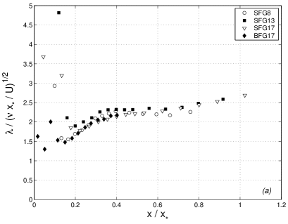
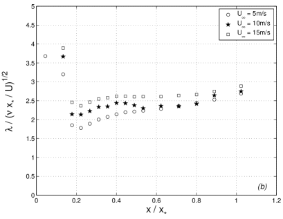
Figure 14: $\lambda/\sqrt{\nu x_{*}/U}$ versus $x/x_{*}$ along the centreline. (a) Data for the four different fractal grids and $U_{\infty}=5.2m/s$. (b) Data for the fractal grid SFG17 and three different inlet velocities $U_{\infty}$.

Before investigating Reynolds number corrections to (34), and therefore (29) which (34) is a direct expression of, we check that the turbulence generated by low-blockage space-filling fractal square grids is indeed fundamentally different from other turbulent flows. For this, we plot $L_{u}/\lambda$ versus $Re_{\lambda}$ in figure 15. Whilst (30), which follows from $\epsilon\sim u^{\prime 3}/L_{u}$, is very well satisfied in turbulent flows not generated by fractal square grids, it is clearly violated by an impressively wide margin in the decay region of turbulent flows generated by low-blockage space-filling fractal square grids. This is not just a matter of a correction to usual laws; it is a matter of dramatically different laws.

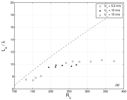
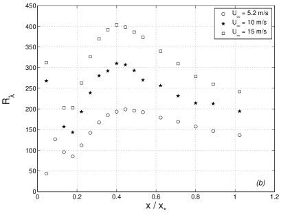
Figure 15: (a) $L_{u}/\lambda$ as a function of $R_{\lambda}$ for different inlet velocities $U_{\infty}$ and different positions on the centreline in the decay region in the lee of the SFG17 fractal grid. The dashed line represents the empirical law obtained by fitting experimental data from various turbulent flows none of which is generated by fractal square grids. This is the data compiled in [25] (which includes jet, regular grid, wake and chunk turbulence), and the dashed line is an excellent representation of $L_{u}/\lambda\sim R_{\lambda}$ particularly at $Re_{\lambda}>150$. (b) $R_{\lambda}$ as a function of $x/x_{*}$ for three different inlet velocities $U_{\infty}$ in the lee of the SFG17 fractal grid.

One important aspect of (30) is that it collapses onto a single curve the $x$ and $Re_{0}$ dependencies of $L_{u}/\lambda$ for many turbulent flows. Figures 16 and 16 show clearly that, in the decay region, $L_{u}/\lambda$ is independent of $x$ and also not significantly dependent on fractal square grid, but is clearly dependent on $U_{\infty}$. There are other turbulent flows where $L_{u}/\lambda$ is independent of $x$, notably plane wakes and axisymmetric jets. However, the important difference is that $Re_{\lambda}$ is also independent of $x$ in plane wake and axisymmetric jet turbulence whereas it is strongly varying with $x$ in turbulent flows generated by fractal square grids (see figure 15). As a result, (30) holds for plane wakes and axisymmetric jets but not for turbulent flows generated by fractal square grids where, instead, $L/\lambda$ is independent of $Re_{\lambda}$ in the decay region (see figure 15), as previously reported in [31]. It is not fully clear from figure 15 if $L/\lambda$ is or is not a constant independent of $Re_{0}$ for large enough values of $Re_{0}$ (specifically for values of $U_{\infty}$ larger or equal to $10m/s$ in the case of 15). The results in [31] might suggest that $L/\lambda$ is independent of $Re_{0}$ for large enough values of $Re_{0}$, but figure 16 does not comfortably support such a conclusion. More data are required for a conclusive assessment of this issue which is therefore left for future study.

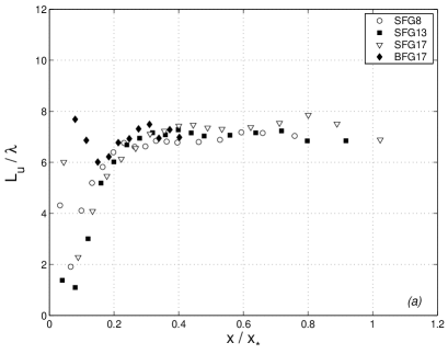
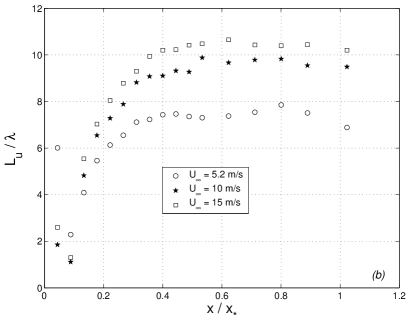
Figure 16: $L_{u}/\lambda$ as a function of $x/x_{*}$ along the centreline (a) for the four different fractal grids and $U_{\infty}=5.2m/s$ and (b) for the fractal grid SFG17 and three different inlet velocities $U_{\infty}$.

We now turn to the Reynolds number corrections which our measurements suggest may be needed in (34). Figures 17 and 17 show that

$$\lambda\sim L_{0}Re_{0}^{-1/3}$$ (35)

is a better approximation than (34) as it collapses the different $U_{\infty}$ data better without altering the quality of the collapse between different fractal grids. From $\epsilon\sim\nu u^{\prime 2}/\lambda^{2}$, (35) implies

$$\epsilon\sim{u^{\prime 2}U_{\infty}\over x_{*}}Re_{0}^{-1/3}$$ (36)

which is an important $Re_{0}$-deviation from (29) and carries with it the extraordinary implication that $\epsilon$ tends to $0$ as $Re_{0}\to\infty$. Of course, this implication is an extrapolation of our results and must be dealt with care. In fact, we show in subsection 4.8, that this extrapolation is actually not supported by our data and the single-length scale theoretical framework of our work.

There is only two ways in which George & Wang’s [12] single-scale theory can account for these deviations from (29) and (34). Either (i) these deviations are an artifact of the different large-scale anisotropy conditions for different values of $Re_{0}$, or (ii) the single-length scale solution of (12) which in fact describes our fractal-generated turbulent flows belongs to the family for which $c\not=0$, not the family for which $c=0$ (see subsection 4.4).

(i) Large-scale anisotropy affects the dimensionless coefficient required to replace the scaling $\nu u^{\prime 2}/\lambda^{2}\sim\epsilon(={3\over 2}B{u^{\prime 2}U_{\infty}\over x_{*}}$ according to (29)) by an exact equality. This issue requires cross-wire measurements at many values of $U_{\infty}$ to be settled and must be left for future study.

(ii) If $c\not=0$, i.e. $c<0$, then

$$u^{\prime 2}={2E_{s}(x_{0})\over 3l(x_{0})}[1+{4\nu a|c|\over l^{2}(x_{0})U_{\infty}}(x-x_{0})]^{(1-c)/2c}$$ (37)

(where we have used $x=U_{\infty}t$ and $x_{0}=U_{\infty}t_{0}$) and (32)-(33) remain valid but with

$$l(x,Re_{0},*)=l(x_{0},Re_{0},*)[1+{4\nu a|c|\over l^{2}(x_{0})U_{\infty}}(x-x_{0})]^{1/2}$$ (38)

not with a length-scale $l$ independent of $x$. Additionally, the following estimates for the Taylor microscale and the dissipation rate $\epsilon$ can be obtained, respectively, from ${d\over dt}u^{\prime 2}\sim\nu u^{\prime 2}/\lambda^{2}$ and from an integration over $\kappa$ of (21):

$$\lambda\sim{l(x_{0},Re_{0},*)\over\sqrt{2a(1-c)}}[1+{4\nu a|c|\over l^{2}(x_{0})U_{\infty}}(x-x_{0})]^{1/2},$$ (39)

$$\epsilon=3\nu a(Re_{0},*)\left(1+|c(Re_{0},*)|\right){u^{\prime 2}\over l^{2}}.$$ (40)

These two equations replace (34) and (29) which follow from $c=0$. It is easily seen that the power-law form (37) tends to the exponential form (25) and that the Taylor microscale $\lambda$ becomes asymptotically independent of $x-x_{0}$ in the limit $c\to 0$.

The new forms (37)-(40) depend on two length-scales, $l(x_{0},Re_{0},*)$ and $x_{0}$, one kinetic energy scale $E_{s}(x_{0})/l(x_{0})$ and two dimensionless numbers, $\nu a(Re_{0},*)/\left(l(x_{0},Re_{0},*)U_{\infty}\right)$ and $c(Re_{0},*)$, all of which may vary with $Re_{0}$ and boundary/inlet conditions. There seems to be enough curve-fitting freedom for these forms to account for our data in the decay regions of our fractal-generated turbulent flows, in particular figures 5b, 6b, 9, 14, 15, 16 and 17. In subsection 4.8 we present a procedure for fitting (37) and (39) to our data which is robust to much of this curve-fitting freedom. It is worth noting here, in anticipation of this subsection, that (39) is consistent with the observation (originally reported in [15] and [31]) that $\lambda$ is approximately independent of $x$ in the decay region, but provided that ${2\nu a|c|\over l^{2}(x_{0})U_{\infty}}(x-x_{0})<<1$ in much of this region. However, (39) also offers a possibility to explain the departure from the constancy of $\lambda$ at large enough values of $x/x_{*}$ where $\lambda$ appears to grow again with $x$ (see figures 14(a) and 17(a)), very much as (39) would qualitatively predict. Note, in particular, that this departure occurs at increasing values of $x/x_{*}$ for increasing $Re_{0}$ (see figures 14(b) and 17(b)) , something which can in principle also be accounted for by (39). In the following subsection we show that same observations can be made for $L_{u}$.

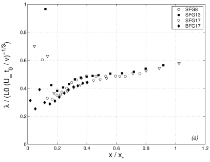
Figure 17: $\lambda/\left(L_{0}({U_{\infty}t_{0}\over\nu})^{-n}\right)$ versus $x/x_{*}$ along the centreline for $n=1/3$ (various values of $n$ were tried and $n=1/3$ offers a clear best fit). (a) Data for the four different fractal grids and $U_{\infty}=5.2m/s$. (b) Data for the fractal grid SFG17 and three different inlet velocities $U_{\infty}$. The results look very similar when plotting $\lambda/\left(L_{0}({Ut_{0}\over\nu})^{-n}\right)$.

4.6 The integral length-scale $L_{u}$

The streamwise evolution of the longitudinal integral length-scale $L_{u}$ on the centreline is plotted in figure 18 for all space-filling fractal square grids as well as for the regular grid SRG. The integral length-scales generated by the fractal square grids are much larger than the regular grid’s even though their effective mesh sizes are smaller. Comparing data from the T-0.46m tunnel, one can see that $L_{u}$ appears independent of the thickness ratio $t_{r}$. However, there are large differences between the integral scales generated by fractal grids SFG17 and BFG17 which have the same $t_{r}$ but fit in different wind tunnels. This observation suggests that the large-scale structure of the fractal grid has a major influence on the integral length-scale. One might in fact expect that the integral length-scale is somehow linked to an interaction length-scale of the grid. For regular grids this interaction length-scale is typically the mesh size, whereas for space-filling fractal square grids a large variety of interaction length-scales exist, the largest being $L_{0}$. Figure 19 supports the view that the scalings of $L_{u}$ and its $x$-dependence are mostly determined by $L_{0}$ and $x_{*}$, respectively, though not perfectly. Figure 19 suggests that $L_{u}/L_{0}$ is not significantly dependent on the inlet Reynolds number $Re_{0}$, at least for the range of $U_{\infty}$ values investigated here. This figure was obtained for the SFG13 grid but is representative of our other three space-filling fractal square grids as well.

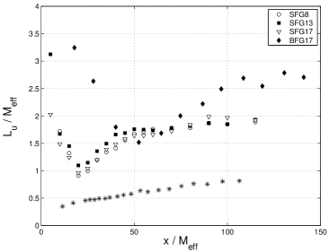
Figure 18: Centreline streamwise evolution of the longitudinal integral length-scale $L_{u}$ normalized by the mesh size $M_{eff}$ ($U_{\infty}=5.2m/s$). Data obtained for the regular grid SRG are also shown ($\star$).

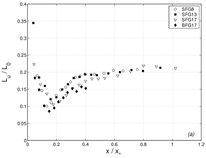
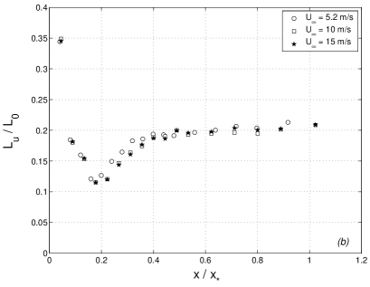
Figure 19: $L_{u}/L_{0}$ as a function of $x/x_{*}$ along the centreline. (a) Four different fractal grids and $U_{\infty}=5.2m/s$. (b) Three different inlet velocities $U_{\infty}$ with the SFG13 fractal grid.

Irrespective of whether $l$ does or does not depend on streamwise coordinate $x$, equations (32) and (33) suggest that $L_{u}/\lambda$ is definitely not a function of $x$ but that it can nevertheless be, in all generality, a function of $Re_{0}$ and of the fractal grid’s geometry. In fact figure 16 is evidence of some dependence on $U_{\infty}$ at least at the lower $U_{\infty}$ values. Assuming $L_{u}\sim L_{0}$ as seems to be suggested by figures 19 and 19 and using either (34) or (35) implies either $L_{u}/\lambda\sim Re_{0}^{1/2}$ or $L_{u}/\lambda\sim Re_{0}^{1/3}$. Of these two implications, it is the latter which agrees best with our measurements (see figures 20 and 20 where we plot $(L_{u}/\lambda)/Re_{0}^{1/3}$ versus $x/x_{*}$) which is consistent with the fact that (35) fits our data better than (34).

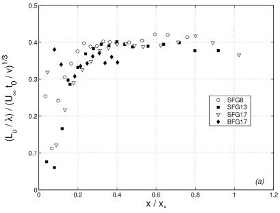
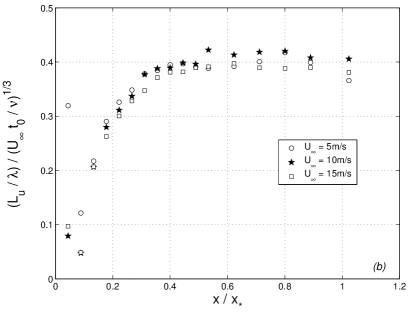
Figure 20: $\left(L_{u}/\lambda\right)/Re_{0}^{1/3}$ as a function of $x/x_{*}$ along the centreline (a) for the four different fractal grids and $U_{\infty}=5.2m/s$ and (b) for the fractal grid SFG17 and three different inlet velocities $U_{\infty}$.

As reported in [15] and [31], $L_{u}$ remains almost constant in the decay region (see figures 19 and 19). The independence on $x$ can be explained in terms of the $c=0$ single-scale solution of George & Wang [12], but it might also be even better explained in terms of the $c<0$ single-scale solution which yields (32) and (38), i.e.

$$L_{u}=\alpha(Re_{0},*)l(x_{0},Re_{0},*)[1+{4\nu a|c|\over l^{2}(x_{0})U_{\infty}}(x-x_{0})]^{1/2}.$$ (41)

A careful examination of figures 19 and 19 suggests that $L_{u}/L_{0}$ may be constant for some of the way downstream in the decay region till it starts increasing slightly, very much like the behaviour of the Taylor microscale $\lambda$ (see figures 14 and 17) and in qualitative agreement with (41). In fact, the ratio $L_{u}/\lambda$ is predicted by (39) and (41) to be independent of $x$ in the decay region, which is in full agreement with figures 16.

The fact that $L_{u}/\lambda$ is independent of x (figure 16) in the decay region where $Re_{\lambda}$ decreases rapidly with increasing $x$ (figure 15b) is evidence against $\epsilon\sim u^{\prime 3}/L_{u}$, not only in the context of $c=0$ single-scale solutions of (12), but also in the context of $c<0$ single-scale solutions of (12). Indeed, (37) and (41) are consistent with $U_{\infty}{d\over dx}u^{\prime 2}\sim-u^{\prime 3}/L_{u}$ only if $c=-1$, in which case $Re_{\lambda}=u^{\prime}\lambda/\nu$ is independent of $x$ because of (37) and (39) and therefore in conflict with our experimental observations and those in [15] and [31]. In fact, the downstream decreasing nature of $Re_{\lambda}$ in the decay region of our fractal-generated turbulent flows imposes $-1<c\leq 0$.

4.7 The energy spectrum $E_{u}(k_{x})$.

The results of subsections 4.4 to 4.6 imply that the small-scale turbulence far downstream of low-blockage space-filling fractal square grids is either fundamentally different from the small-scale turbulence in documented boundary-free shear flows and decaying wind tunnel turbulence originating from a regular/active grid, or $\epsilon\sim u^{\prime 3}/L_{u}$ does not hold in these non-fractal-generated flows where the length-scale ratio $L_{u}/\lambda$ is proportional to $Re_{\lambda}$ if one assumes $\epsilon\sim u^{\prime 3}/L_{u}$. Our results therefore shed serious doubt on the universality of $\epsilon\sim u^{\prime 3}/L_{u}$, the cornerstone assumption present either explicitely or implicitely in most if not all turbulence models and theories [1], [34], [9], [29], [30].

However, our data do not allow us to educe with full confidence a formula for the dissipation rate $\epsilon$ in turbulence generated by space-filling fractal square grids. This issue is related to the fact that whilst an exponential turbulence decay (equations 10 and 11) fits our data well, the $Re_{0}$ dependence of $\lambda$ which follows from it in a self-preserving single-length scale context does not. Qualitative observations of the x-dependence of $L_{u}$ and $\lambda$ may suggest that the turbulence decay is in fact a power-law of the type (37), rather than exponential, albeit with a power-law exponent large enough (i.e. $c$ close enough to 0) for the exponential form to be a good fit. An attempt at addressing this issue is made in the following and final subsection 4.8. This attempt relies on the results of our examination of energy spectra and the single-length scale assumption which we now report.

Seoud & Vassilicos [31] studied the downstream evolution of the 1D energy spectrum $E_{u}(k_{x},x)$ in the decay region of space-filling fractal square grids and found that, for a given velocity $U_{\infty}$, $E_{u}(k_{x},x)$ can be collapsed for different downstream positions and for all our fractal grids in terms of (31) where $l$ is replaced by either $\lambda$ or $L_{u}$. Indeed, $E_{u}(k_{x})=u^{\prime 2}\lambda F_{u}(k_{x}\lambda)$ and $E_{u}(k_{x})=u^{\prime 2}L_{u}F_{u}(k_{x}L_{u})$ collapse the entire spectral data equally well at a given inlet velocity $U_{\infty}$, a fact which we confirm in figures 21, 21, 22 and 22. These figures clearly support George & Wang’s [12] single-length scale assumption (16) and (31).

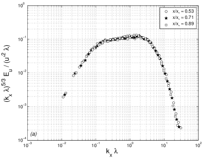
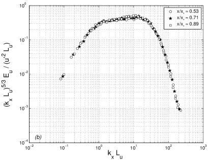
Figure 21: SFG17 grid in the T-0.46 tunnel with $U_{\infty}=5.2m/s$ along the centreline. Compensated 1D energy spectra normalized using (a) $u^{\prime 2}$ and $\lambda$ or (b) $u^{\prime 2}$ and $L_{u}$. Spectra from different centreline positions $x/x_{*}$ collapse over all wavenumbers.

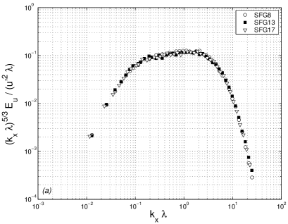
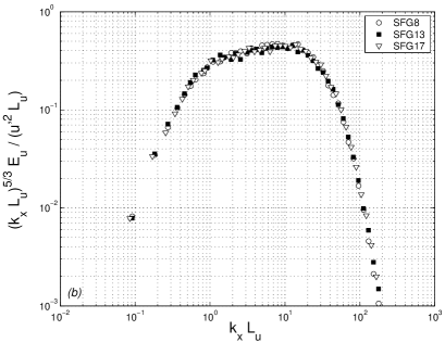
Figure 22: T-0.46 tunnel with $U_{\infty}=5.2m/s$ along the centreline. Compensated 1D energy spectra measured at $x/x_{*}=0.62$ and normalized using (a) $u^{\prime 2}$ and $\lambda$ or (b) $u^{\prime 2}$ and $L_{u}$. Spectra corresponding to our different grids appear to collapse over all wavenumbers.

However, Seoud & Vassilicos [31] did not attempt to collapse energy spectra for different inlet velocities $U_{\infty}$. We therefore compare energy spectra obtained at the same position downstream of the same fractal grid but with different inlet velocities $U_{\infty}$. In figures 23 and 23 we report such results obtained at $x/x_{\star}\approx 0.62$ with the SFG17 grid. These figures are representative of all other such results which we obtained with our other fractal grids and at other positions but which we do not present here for economy of space.

From these figures, the form $E_{u}(k_{x})=u^{\prime 2}\lambda F_{u}(k_{x}\lambda)$ may seem to offer a much better collapse for different inlet velocities $U_{\infty}$ than $E_{u}(k_{x})=u^{\prime 2}L_{u}F_{u}(k_{x}L_{u})$. The discrepancy of the form $E_{u}(k_{x})=u^{\prime 2}L_{u}F_{u}(k_{x}L_{u})$ is mostly at the high wavenumbers and is made evident by our compensation of the spectra by $(k_{x}L_{u})^{5/3}$. It might be tempting to conclude that $l$ is different from $L_{u}$ and in fact equal to $\lambda$, but such a conclusion would be incompatible with $E_{u}(k_{x})=u^{\prime 2}\lambda F_{u}(k_{x}\lambda)$ because (32) and (33) would then lead to the inconsistency that $l$ is in fact not different from $L_{u}$. The fact that $L_{u}/\lambda$ grows with $Re_{0}$, at least for the range of $Re_{0}$ values considered here, suggests that we should be considering a spectral form $E_{u}(k_{x})=u^{\prime 2}lF_{u}(k_{x}l,Re_{0},*)$ without neglecting the dependencies on $Re_{0}$ and perhaps even $*$.

We have seen in the previous subsection that much of the scaling of $L_{u}$ is controlled by $L_{0}$, i.e. $L_{u}\sim L_{0}$ to a first scaling approximation, and that $L_{u}$ does not vary significantly with $U_{\infty}$. Figure 23 suggests that the plot of $E_{u}(k_{x})/\left(u^{\prime 2}L_{u}\right)$ versus $k_{x}L_{u}$ is also imperceptibly dependent on $U_{\infty}$ at the lower values of $k_{x}L_{u}$ but not at the higher ones. These three observations can all be explained if the assumption is made that

$$l(x_{0},Re_{0},*)=L_{0}$$ (42)

and that

$$F_{u}(k_{x}l,Re_{0},*)=f_{u}(k_{x}l)H_{u}(k_{x}lRe_{0}^{-n})$$ (43)

where $n>0$ and $H_{u}$ is a monotonically decreasing function which is very close to 1 where $k_{x}lRe_{0}^{-n}<1$ and very close to 0 where $k_{x}lRe_{0}^{-n}>1$. There may be residual dependencies on the geometry of the fractal grid, i.e. on $*$, but we do not have enough fractal grids in our disposal to determine them. Once again, this is an issue for future study.

Equations (31), (38), (42) and (43) can readily account for the behaviour observed in figure 23. Combined with (32), (42) and (43) also imply that $L_{u}$ scales with $L_{0}$ provided that $f_{u}$ is a decreasing function of $k_{x}l$ where $k_{x}l>1$. Figures 20 and 20 would then suggest that $\beta$ in (33) scales as $Re_{0}^{-1/3}$. It is the function $H_{u}(k_{x}lRe_{0}^{-n})$ in (43) which makes this scaling possible. In fact, if $f_{u}\sim(k_{x}l)^{-p}$ where $k_{x}l>1$, then (33), (38) and (42) imply $\lambda\sim L_{0}Re_{0}^{-n(3-p)/2}$. Note that the Kolmogorov-like exponents $p=5/3$ and $n=3/4$ (see [29], [34], [9]) yield $\lambda\sim L_{0}Re_{0}^{-1/2}$ identically to (34) which follows from the $c=0$ single-length scale solution of the spectral energy equation (12).

The good collapse in terms of both forms $E_{u}(k_{x})=u^{\prime 2}\lambda F_{u}(k_{x}\lambda)$ and $E_{u}(k_{x})=u^{\prime 2}L_{u}F_{u}(k_{x}L_{u})$ in figures 21 and 21 comes from the fact that all data in these figures are obtained for the same value of $Re_{0}$ and the same fractal grid, and that $L_{u}/\lambda$ does not vary with $x$. These figures are therefore also consistent with (42) and (43). The good collapse of the form $E_{u}(k_{x})=u^{\prime 2}L_{u}F_{u}(k_{x}L_{u})$ in figure 22 is mainly a consequence of the fact that the fractal grids SFG8, SFG13 and SFG17 all have the same value of $L_{0}$ and can also follow from (42) and (43). However, the apparently good collapse of the form $E_{u}(k_{x})=u^{\prime 2}\lambda F_{u}(k_{x}\lambda)$ in figure 22 must be interpreted as being an artifact of the limited range of values of thicknesses $t_{0}$ that we have experimented with (see table 1), more limited than the range of inlet velocities $U_{\infty}$ which allows the $Re_{0}^{1/3}$ scaling of $L_{u}/\lambda$ to be picked up by our spectra in figure 23 but not in figure 22.

Returning to figure 23 we notice that it does not, in fact, present such a good collapse of the data, particularly over the range of scales where the collapse in figure 23 appears good. Within the framework of (42) and (43), the semblance of a perhaps acceptable collapse in figure 23 results from a numerical circumstance to do with the exponents $n$ and $p$. Chosing $p=5/3$ and $n=3/4$ for the sake of argument, (31),(38), (42) and (43) would imply that the quantity plotted in this figure, i.e. $(k_{x}\lambda)^{5/3}E_{u}(k_{x})/\left(u^{\prime 2}\lambda\right)$, is in fact equal to $Re_{0}^{-1/3}H_{u}(k_{x}\lambda Re_{0}^{-1/9})$ in the range which would correspond to $k_{x}\lambda\geq 0.1$ in the figure. Over the range of inlet velocities tried here, $Re_{0}^{-1/9}$ remains about constant whilst $Re_{0}^{-1/3}$ varies a bit thus producing the effect seen in figure 23: a slight dependence on $U_{\infty}$ of the plateau and a semblance of a collapse of the dissipative range of the spectra.

The conclusion of this data analysis is that the self-preserving spectral form

$$E_{u}(k_{x})=u^{\prime 2}lf_{u}(k_{x}l)H_{u}(k_{x}lRe_{0}^{-n})$$ (44)

with

$$l=L_{0}[1+{4\nu a|c|\over L_{0}^{2}U_{\infty}}(x-x_{0})]^{1/2}$$ (45)

is consistent with the theory of George & Wang [12] and with our measurements in the decay region in the lee of our fractal square grids. We must stress again that future work is required with a wider range of fractal grids, measurement positions and inlet velocities in order to reach definitive conclusions confidently valid over a wider range of parameters.

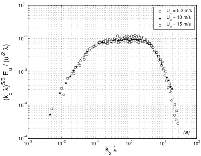
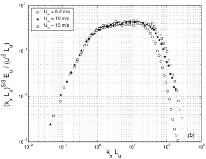
Figure 23: SFG17 in the T-0.46 tunnel. (a) Compensated 1D energy spectra normalized by the Taylor micro-scale $\lambda$. (b) Compensated 1D energy spectra normalized by the large-scale properties measured on centreline downstream fractal grid SFG17 for different inlet velocities $U_{\infty}$ ($x/x_{\star}\approx 0.62$ on the centreline).

4.8 Exponential versus power-law turbulence decay.

We close section 4 with a discussion of how the exponential turbulence decay (25) corresponding to the $c=0$ solution and the power-law turbulence decay (37)-(38)-(39) corresponding to $-1<c<0$ solutions might fit together into a single framework. We already commented straight under equation (40) that the power-law form (37) tends to the exponential form (25) and that the Taylor microscale $\lambda$ becomes asymptotically independent of $x-x_{0}$ in the limit $c\to 0$. We now attempt to fit expression (37) to our decay region data and compare it with our exponential fit (10) (which is consistent with (25) and (26)). To do this we start by fitting (39) to our Taylor microscale decay region data using some of the results reached in the previous subsection for our range of experimental parameters, namely $\beta\sim Re_{0}^{-1/3}$ and $l(x_{0})=L_{0}$. We therefore reformulate (39) as follows:

$$\frac{\lambda^{2}}{L_{0}^{2}Re_{0}^{-2/3}}=1+\gamma\left(\frac{x-x_{0}}{x_{\star}}\right)$$ (46)

where

$$\gamma=\frac{4a\left|c\right|}{Re_{0}}.$$ (47)

We have, in effect, arbitrarily set to 1 a $Re_{0}$-independent dimensionless parameter (or, if $\beta\sim Re_{0}^{-1/3}$ is somewhat faulty, perhaps even a weakly $Re_{0}$-dependent parameter) multiplying the left hand side of (46). However, most of the potential $Re_{0}$-dependence remains intact in this relation, in particular as $\gamma$ is a priori $Re_{0}$-dependent.

Relation (46) is plotted in Fig. 24 for the SFG17 grid and for all our inlet velocities $U_{\infty}$. From these curves it is easy to estimate $\gamma$ independently of the virtual origin $x_{0}$, and we report our results in table 5.

$U_{\infty}[m/s]$	$5.2m/s$	$10m/s$	$15m/s$
$\gamma$	$0.23$	$0.2$	$0.13$

Table 5: Estimates of the coefficient $\gamma$ for the grid SFG17.

We can now attempt to fit (37) to our turbulence decay data. Equation (37) can be recast in the form

$$\ln{\left(u^{\prime 2}\right)}=\ln{\left(\frac{2E_{s}(x_{0})}{3l(x_{0})}\right)}+\frac{1-c}{2c}\ln{\left[1+\frac{4\nu a\left|c\right|}{l(x_{0})^{2}U_{\infty}}\left(x-x_{0}\right)\right]}.$$ (48)

The observed near-constancies of $\lambda$ and $L_{u}$ in the decay region suggest from (39) and (41) that $\frac{4\nu a\left|c\right|}{l(x_{0})^{2}U_{\infty}}\left(x-x_{0}\right)<<1$. It is therefore reasonable to consider the first order approximation of (48), which is

$$\ln{\left(u^{\prime 2}\right)}\approx\ln{\left(\frac{2E_{s}(x_{0})}{3l(x_{0})}\right)}+\left(\frac{1-c}{2c}\right)\left[\frac{4\nu a\left|c\right|}{l(x_{0})^{2}U_{\infty}}\left(x-x_{0}\right)\right]$$ (49)

and which can be reformulated as

$$\ln{\left(u^{\prime 2}\right)}\approx\ln{\left(\frac{2E_{s}(x_{0})}{3l(x_{0})}\right)}+\delta\left(\frac{x-x_{0}}{x_{\star}}\right)$$ (50)

with $\delta=\left(\frac{1-c}{2c}\right)\gamma$. This linear formula makes it easy to determine $\delta$ from our experimental data independently of $E_{s}(x_{0})/l(x_{0})$ and $x_{0}$, as indeed shown in figure 24 where (50) actually appears to fit our data well for all inlet velocities $U_{\infty}$. Our resulting best estimates of the dimensionless parameter $\delta$ are reported in table 6. This parameter appears to be $Re_{0}$-independent, in agreement with the $Re_{0}$-independence of the turbulence intensity reported in figure 6.

$U_{\infty}[m/s]$	$5.2m/s$	$10m/s$	$15m/s$
$\delta$	$-2.3$	$-2.2$	$-2.4$

Table 6: Estimates of the coefficient $\delta$ for the grid SFG17.

The dimensionless coefficients $a$ and $c$ can now be obtained from our estimates of $\gamma$ and $\delta$ using $c=\frac{\gamma}{2\delta+\gamma}$ and

$$a={Re_{0}\over 2}|\delta+\gamma/2|.$$ (51)

In table 7 we list the values thus obtained for $c$ and $a$. It is rewarding to see that $c$ turns out to be negative and in fact larger than $-1$. Of particular interest is the finding that $c\to 0$ with increasing $Re_{0}$ and that the values of $c$ are indeed quite close to $0$ for all our inlet velocities. These results suggest that the single-length scale power-law turbulence decay (37) tends towards the exponential turbulence decay (25) with the dimensionless coefficient $a$ given by (51). Equation (51) is in fact equivalent to equation (26) which we obtained by fitting our turbulence intensity data with an exponential decay form. The Taylor microscale $\lambda$ also tends to an $x$-independent form with increasing $Re_{0}$ because $\gamma\to 0$, and so does

$$L_{u}=\alpha L_{0}\left[1+\gamma(x-x_{0})/x_{*}\right]^{1/2}$$ (52)

(obtained from (41) and (42)). Indeed, we have checked that, in the decay regions of our fractal-generated turbulent flows, (52) provides a good fit of our $L_{u}$ data with the same values of $\gamma$ as the ones listed in table 5 and with a dimensionless constant ($\alpha\approx 0.34$ in the case of the SFG17 grid) for all our inlet velocities $U_{\infty}$.

The dissipation rate $\epsilon$ is given by (40) in the context of the power-law decaying single-length scale turbulence and it is easy to check that (40) tends to (29), the dissipation rate form of the $c=0$ exponentially decaying single-length scale turbulence, as $Re_{0}$ increases. Of course, this assumes that $\gamma$ and $c$ tend to $0$ in that limit as the extrapolation of our fits would suggest. Equation (36) is incompatible with the view that power-law decaying single-length scale turbulence tends towards exponentially decaying single-length scale turbulence in the limit $Re_{0}\to\infty$.

Similarly, the empirical scaling of equation (35), i.e. $\lambda\sim L_{0}Re_{0}^{-1/3}$, is also incompatible with such a gradual asymptotic behaviour. If use is made of (51), or equivalently (26), equation (39) shows that, as $Re_{0}$ grows, $\lambda$ tends towards $\lambda\sim L_{0}Re_{0}^{-1/2}$, the form predicted by the exponentially decaying single-length scale solution (see equation (34) and the argument leading to it).

We noted in the previous subsection that an energy spectrum with a power-law intermediate range, i.e. $f_{u}\sim(k_{x}l)^{-p}$ where $k_{x}l>1$, and a spectral form (31) with (43), (38) and (42) implies $\lambda\sim L_{0}Re_{0}^{-n(3-p)/2}$. We also noted that the Kolmogorov-like exponents $n=3/4$ and $p=5/3$ yield $\lambda\sim L_{0}Re_{0}^{-1/2}$. We are now suggesting that fits of the exponent $n(3-p)/2$ might tend to $1/2$ as $Re_{0}$ increases. This seems consistent with our observation that fits of the intermediate form $f_{u}\sim(k_{x}l)^{-p}$ to our spectral data lead to $p=1.50$ for $U_{\infty}=5m/s$, $p=1.57$ for $U_{\infty}=10m/s$ and $p=1.60$ for $U_{\infty}=15m/s$ (see figure 25). The exponent $p$ might indeed be tending towards $5/3$ with increasing $Re_{0}$, in which case we might also expect the exponent $n$ to tend towards $3/4$ if $n(3-p)/2$ tends to $1/2$.

$U_{\infty}[m/s]$	$5.2m/s$	$10m/s$	$15m/s$
$c$	$-0.053$	$-0.048$	$-0.028$
$a$	$20.6$	$24.6$	$31.3$

Table 7: Estimates of the coefficients $a$ and $c$ for the grid SFG17.

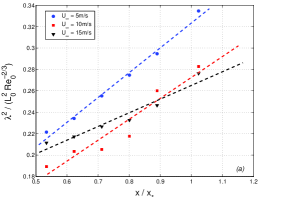
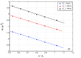
Figure 24: SFG17 grid in the T-0.46m tunnel with three different inlet velocities. (a) Fit (46) of centreline $\lambda$ data. (b) Fit (50) of centreline $u^{\prime 2}$ data.

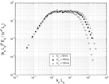
Figure 25: $(k_{x}L_{u})^{p}E_{u}(k_{x})/\left(u^{\prime 2}L_{u}\right)$ versus $k_{x}L_{u}$ for the value of the exponent $p$ which gives the most horizontal plateau. Data obtained with the SFG17 grid at $x/x_{*}=0.62$ on the centreline of the T-0.46m tunnel with three different inlet velocities. The exponent $p$ seems to increase towards $5/3$ with increasing $U_{\infty}$ ($p=1.50$ for $U_{\infty}=5.2m/s$, $p=1.57$ for $U_{\infty}=10m/s$, $p=1.60$ for $U_{\infty}=15m/s$).

5 Conclusions and issues raised

There are two regions in turbulent flows generated by the low blockage space-filling fractal square grids experimented with here. The production region between the grid and a distance about $0.5x_{*}$ from it and the decay region beyond $0.5x_{*}$. In the production/decay region the centreline turbulence intensity increases/decreases in the downstream direction. The wake-interaction length-scale $x_{*}$ is determined by the large scale features of our fractal grids, $x_{*}=L_{0}^{2}/t_{0}$, but it must be kept in mind that one cannot change $t_{0}$ and or $L_{0}$ without changing the rest of the fractal structure of these fractal grids. The downstream evolution of turbulence statistics scales on $x_{*}$ and can be collapsed with it for all our grids. However, it must be stressed that we have tested only four fractal grids from a rather restricted class of multiscale/fractal grids and we caution against careless extrapolations of the role of this wake-interaction length-scale to other fractal grids. For example, Hurst & Vassilicos [15] experimented with a low $t_{r}$ space-filling fractal square grid which seemed to produce two consecutive peaks of turbulence intensity instead of one downstream of it. A wider range of wake-interaction length scales should probably be taken into account for such a fractal grid, an issue which needs to be addressed in future work on fractal-generated turbulence.

Whilst the turbulence in the production region is very inhomogeneous with non-gaussian fluctuating velocities, it becomes quite homogeneous with approximately gaussian fluctuating velocities in the decay region. Unlike turbulence decay in boundary-free shear flows and regular grid-generated wind tunnel turbulence where $L_{u}/\lambda$ and $Re_{\lambda}$ change together so that their ratio remains constant, in the decay region of our fractal-generated turbulent flows $L_{u}/\lambda$ remains constant and $Re_{\lambda}$ decreases as the turbulence decays. This very unusual behaviour implies that $L_{u}/\lambda\sim Re_{\lambda}$ and the Richardson-Kolmogorov cascade are not universal to all boundary-free weakly sheared/strained turbulence. In turn, this implies that $\epsilon\sim u^{\prime 3}/L_{u}$ is also not universally valid, not even in homogeneous turbulence as our fractal-generated turbulence is approximately homogeneous in the decay region. Inlet/boundary conditions seem to have an impact on the relation between $L_{u}/\lambda$ and Reynolds number. The issue which is now raised for future studies is to determine what it is in the nature of inlet conditions and turbulence generation that controls the relation between the range of excited turbulence scales and the levels of turbulence kinetic energy. Whilst the general form $L_{u}/\lambda=Re_{0}^{1/2}fct({x-x_{0}\over L_{B}})$ may be universal, including fractal-generated turbulent flows, the actual function of ${x-x_{0}\over L_{B}}$ in this form is not and can even be of a type which does not allow to collapse the $x$ and $Re_{0}$ dependencies by the Richardson-Kolmogorov cascade form $L_{u}/\lambda\sim Re_{\lambda}$.

This issue certainly impacts on the very turbulence interscale transfer mechanisms, in particular vortex stretching and vortex compression which are considered to have qualitatively universal properties such as the tear drop shape of the Q-R diagram [35]. Multi-hot wire anemometry [14] applied to turbulence generated by low-blockage space-filling fractal square grids may have recently revealed very unusual Q-R diagrams without clear tear-drop shapes [17]. Fractal-generated turbulence presents an opportunity to understand these interscale transfer mechanisms because it offers ways to tamper with them.

The decoupling between $L_{u}/\lambda$ and $Re_{\lambda}$ can be explained in terms of a self-preserving single-length scale type of decaying homogeneous turbulence [12] but not in terms of the usual Richardson-Kolmogorov cascade ([1], [9], [29], [30]) and its cornerstone property, $\epsilon\sim u^{\prime 3}/L_{u}$. This self-preserving single-scale type of turbulence allows for $L_{u}/\lambda$ to increase with inlet Reynolds number $Re_{0}$, as we in fact observe. This is a case where the range of excited turbulence scales depends on a global Reynolds number but not on the local Reynolds number.

Our data support the view (both its assumptions and consequences) that decaying homogeneous turbulence in the decay region of some low-blockage space-filling fractal square grids is a self-preserving single-length scale type of decaying homogeneous turbulence [12]. Furthermore, our detailed analysis of our data suggests that such fractal-generated turbulence might be extrapolated to have the following specific properties at high enough inlet Reynolds numbers $Re_{0}$:

$$E_{u}(k_{x},x)=u^{\prime 2}(x)L_{0}(k_{x}L_{0})^{-5/3}H_{u}(k_{x}L_{0}Re_{0}^{-3/4}),$$ (53)

$$u^{\prime 2}(x)\approx u_{0}^{\prime 2}e^{-2x/x_{*}},$$ (54)

$$\epsilon\approx 3u^{\prime 2}U_{\infty}/x_{*},$$ (55)

$$L_{u}\sim L_{0}$$ (56)

and

$$\lambda\sim L_{0}Re_{0}^{-1/2}$$ (57)

where both $L_{u}$ and $\lambda$ are independent of $x$. A more detailed account of our conclusions involves the two types of single-scale solutions of the spectral energy equation, the $c=0$ and the $-1<c<0$ types introduced in subsections 4.4 and 4.5. In subsection 4.8 we showed how our data indicate that the turbulence in the decay region is of the $-1<c<0$ type with a value of $c$ which tends to $0$ as $Re_{0}$ increases. This is why we stress the asymptotic extrapolations (53), (54), (55) and (57) in this conclusion.

Our data require a very clear departure from the usual views concerning high Reynolds number turbulence [1], [9], [21], [29], [30], [34]. There is definitely a need to investigate these suggested high-$Re_{0}$ properties further. Measurements with a wider range of fractal grids and a wider range of inlet velocities in perhaps a wider range of wind tunnels and with a wider range of measurement apparatus: x-wires, multi-hot wire anemometry [14], [17] and particle image velocimetry. Direct Numerical Simulations (DNS) of fractal-generated turbulent flows are only now starting to appear [28], [18] and their role will be crucial. Amongst other things, these studies will reveal dependencies on inlet/boundary geometrical conditions $*$ which we have not been able to fully determine here because of the limited range of fractal grids at our disposal.

A quick discussion of the features of extrapolations (53)-(57) reveals the various issues that they raise. The first issue which immediately arises is the meaning of $Re_{0}\to\infty$. We cannot expect this limit to lead to (53)-(57) if it is not taken by also increasing the number $N$ of iterations on the fractal turbulence generator. How do our results and the extrapolated forms (53)-(57) depend on $N$?

Secondly, in the extrapolated spectral form (53) we have assumed that the exponent $p$ tends to $5/3$ in the high-$Re_{0}$ limit and have therefore, in particular, neglected to consider any traditional small-scale intermittency corrections (see [9]). This may be consistent with the observation of Stresing et al [33] that small-scale intermittency is independent of $Re_{\lambda}$ in the decay region of our flows. However it is not clear why $p$ should asymptotically equal $5/3$ in the non-Kolmogorov context of our self-preserving single-scale decaying homogeneous turbulence. In particular, the inner length-scale $L_{0}Re_{0}^{-3/4}$ differs from the Kolmogorov microscale $\left(\nu^{3}/\epsilon\right)^{1/4}$ which scales as $L_{0}Re_{0}^{-3/4}(t_{0}/L_{0})^{1/2}(u^{\prime}/U_{\infty})^{-1/2}$ if account is taken of (55). If $L_{0}Re_{0}^{-3/4}$ in (53) was to be replaced by this Kolmogorov microscale, then (57) would fail and the single-length scale framework of George & Wang [12] would fail with it. Why is the Kolmogorov microscale absent, or at least apparently absent, from decaying homogeneous turbulence in the decay region of some low-blockage space-filling fractal square grids?

Thirdly, (55) suggests that the kinetic energy dissipation rate per unit mass is proportional to $u^{\prime 2}$ rather than $u^{\prime 3}$ and that the turnover time scale is the global $x_{*}/U_{\infty}$ rather than the local $L_{u}/u^{\prime}$. What interscale transfer mechanisms cause one or the other dependencies, and what are the implied changes in the vortex stretching and vortex compression mechanisms hinted at by the recent preliminary Q-R diagram results of Kholmyansky and Tsinober [17]? These issues directly address the universality questions raised in the Introduction and depend on the mechanisms of turbulence generation in the production region and the mechanisms which force important features of particular turbulence generations to be or not to be remembered far downstream from the initial generator. What is the role of coherent structures, large or small, in shaping the type of homogeneous turbulence which decays freely in the decay region?

Fourthly, is it possible that turbulence in various instances in industry and nature (e.g. in or over forest canopies, coral reefs, complex mountainous terrains, etc) might appear as a mixture of single-scale self-preserving turbulence and Richardson-Kolmogorov turbulence? Could such mixtures of two types of different turbulence give rise to what may appear as Reynolds number and intermittency corrections to the usual Richardson-Kolmogorov phenomenology and scalings?

As a final note, it is worth comparing (55) with the usual estimate $\epsilon=C_{\epsilon}u^{\prime 3}/L_{u}$, which can also be seen as a general definition of the dissipation constant $C_{\epsilon}$. One gets

$$C_{\epsilon}\approx{3\over 5}{(t_{0}/L_{0})\over(u^{\prime}/U_{\infty})}$$ (58)

where use has been made of the estimate $L_{u}\approx 0.2L_{0}$ extracted from figures 19. The dissipation constant $C_{\epsilon}$ is not only clearly not universal, it can also be given bespoke values by designing the geometry of the turbulence-generating fractal grid, i.e. by changing the aspect ratio $t_{0}/L_{0}$. Furthermore, whilst a constant and universal value of $C_{\epsilon}$ would imply that, given a value of $L_{u}$, the level of turbulence dissipation cannot come without an equivalent pre-determined level of turbulence fluctuations, (55) and (58) show that it actually is possible to generate an intense turbulence with reduced dissipation and even design the level of this dissipation. The implications for potential industrial flow applications are vast and include energy-efficient mixers (see [6]) and lean premixed combustion gas turbines on which we will report elsewhere.

Acknowledgements: We acknowledge Mr Carlo Bruera’s and Mr Stefan Weitemeyer’s assistance with the anemometry data collection.

References

- [1] G.K. Batchelor, The Theory of Homogeneous Turbulence, Cambridge University Press, (1953)
- [2] G.K. Batchelor & A.A. Townsend, Decay of isotropic turbulence in the initial period, Proc. Roy. Soc. A, vol. 193(1035), 539-558, 1948
- [3] J.C. Bennett & S. Corrsin, Small Reynolds number nearly isotropic turbulence in a straight duct and a contraction, Phys. Fluids, vol. 21(12), 2129-2140, 1978
- [4] R. Betchov, On the fine structure of turbulent flows, J. Fluid Mech., vol. 3(2), 205-216, 1957
- [5] P.M. Bevilaqua & P.S. Lykoudis, Turbulence memory in self-preserving wakes, J. Fluid Mech. vol. 89(3), 589-606, 1978
- [6] C.J. Coffey, G.R. Hunt, R.E. Seoud & J.C. Vassilicos, Mixing effectiveness of fractal grids for inline static mixers, Experimental Thermal and Fluid Science (submitted 1 July 2009).
- [7] G. Comte-Bellot & S. Corrsin, The use of a contraction to improve the isotropy of grid-generated turbulence, J. Fluid Mech., vol. 25, part 4, 657-682, 1966
- [8] S. Corrsin, Turbulence : Experimental methods, In Handbook der Physik, Springer, New York, (1963)
- [9] U. Frisch, Turbulence. The Legacy of A.N. Kolmogorov., Cambridge University Press, (1995)
- [10] M. Gad-El-Hak & S. Corrsin, Measurements of the nearly isotropic turbulence behind a uniform jet grid, J. Fluid Mech., vol. 62(1), 115-143, 1974
- [11] W.K. George, Is there an asymptotic effect of initial and upstrean conditions on turbulence?, Proc. ASME 2008 Fluid Engineering Meeting, 2008 Freeman Lecture, August 10-14, 2008, Jacksonville, Florida, USA.
- [12] W.K. George & H. Wang, The exponential decay of homogeneous turbulence, Phys. Fluids, vol. 21, 025108, 2009
- [13] S. Goto & J.C. Vassilicos, The dissipation rate coefficient of turbulence is not universal and depends on the internal stagnation point structure. Phys. Fluids vol. 21, 035104, 2009
- [14] G. Gulitski, M. Kholmyansky, W. Kinzelbach, B. L?thi, A. Tsinober & S. Yorish, Velocity and temperature derivatives in high-Reynolds-number turbulent flows in the atmospheric surface layer. Part 1. Facilities, methods and some general results, J. Fluid Mech. vol. 589, 57, 2007
- [15] D. Hurst & J.C. Vassilicos, Scalings and decay of fractal-generated turbulence, Phys. Fluids, vol. 19, 035013, 2007
- [16] H. Kahalerras, Y. Malecot, Y. Gagne & B. Castaing, Intermittency and Reynolds number, Phys. Fluids, 10(4), 910-921, 1997
- [17] M. Kholmyansky, A. Tsinober, Processing of the data measured in the Department of Aeronautics of Imperial College of Science, Technology and Medicine, Report on Research Project. Tel Aviv University, May 2009.
- [18] S. Laizet, E. Lamballais & J.C. Vassilicos, A numerical strategy to combine high-order schemes, complex geometry and massively parallel computing for the DNS of fractal-generated turbulence, Computers and Fluids vol. 39(3), 471-484, 2010.
- [19] S. Laizet & J.C. Vassilicos, Direct numerical simulation of fractal-generated turbulence, In Proc. 7th ERCOFTAC Workshop on Direct and Large-Eddy Simulation, Trieste, Italy, September 2008. Springer, 2009
- [20] P. Lavoie, P. Burratini, L. Djenidi & R. A. Antonia, Effect of initial conditions on decaying grid turbulence at low , Exp. Fluids, vol. 39(5), 2005
- [21] M. Lesieur, Turbulence in Fluids, Springer, (2008)
- [22] H. Makita, Realization of a large-scale turbulence field in a small wind tunnel, Fluid Dyn. Res., vol. 8, 53-64, 1991
- [23] J. Mathieu & E. Alcaraz Réalisation d’une soufflerie à haut niveau de turbulence, Comtes Rendus, vol. 261, 2435.
- [24] M.R. Maxey, The velocity skewness in grid turbulence, Phys. Fluids, vol. 30(4), 935-938, 1987
- [25] N. Mazellier & J.C. Vassilicos, The turbulence dissipation constant is not universal because of its universal dependence on large-scale flow topology, Phys. Fluids, vol. 20, 015101, 2008
- [26] M.S. Mohamed & J.C. LaRue, The decay power-law in grid-generated turbulence, J. Fluid Mech., vol. 219, 195-214, 1990
- [27] L. Mydlarski & Z. Warhaft, On the onset of high-Reynolds-number grid-generated wind tunnel turbulence, J. Fluid Mech., vol. 320, 331-368, 1996
- [28] K. Nagata, H. Suzuki, Y. Sakai, T. Hayase, & T. Kubo, DNS of passive scalar field with mean gradient in fractal-generated turbulence, Int. Rev. Phys., vol. 2 (5), 2008.
- [29] S.B. Pope, Turbulent Flows, Cambridge University Press, (2000)
- [30] P. Sagaut & C. Cambon, Homogeneous Turbulence Dynamics, Cambridge University Press, (2008)
- [31] R.E. Seoud & J.C. Vassilicos, Dissipation and decay of fractal-generated turbulence, Phys. Fluids, vol. 19, 105108, 2007
- [32] K.R. Sreenivasan & R.A. Antonia, The phenomenology of small-scale turbulence, Ann. Rev. Fluid Mech. 29, 435-72, 1997
- [33] R. Stresing, J. Peinke, R.E. Seoud & J.C. Vassilicos, Fractal-generated turbulence - a new class of turbulent flows? Phys. Rev. Lett. (submitted).
- [34] H. Tennekes & J.L. Lumley, A First Course In Turbulence., MIT Press, (1972)
- [35] A. Tsinober, An Informal Conceptual Introduction to Turbulence, Springer, (2009)
- [36] C. Tong & Z. Warhaft, Turbulence suppression in a jet by means of a fine ring, Phys. Fluids, vol. 6, 328, 1994
- [37] A.A. Townsend, The structure of turbulent shear flows, Cambridge University Press, (1956)
- [38] R. Vonlanthen & P.A. Monkewitz, A new passive turbulence grid with improved isotropy, American Physical Society, 61st Annual Meeting of the APS Division of Fluid Dynamics, November 23-25, 2008, abstract MB.004.