Planetary Dynamics and Habitable Planet Formation In Binary Star Systems

1 Introduction

How our planet was formed, how life came about, and whether life exists elsewhere in the universe are among some of the long-standing questions in human history. The latter, which has been the main drive behind many decades of searching for planets outside the solar system, is one of the most outstanding problems in planetary science and astrobiology. Although no Earth-like planet has yet been found, the success of observational techniques in identifying now more than 350 extrasolar planets has greatly contributed to addressing this question, and has extended the concept of habitability to billions of miles beyond the boundaries of our solar system. It is now certain that our planetary system is not unique and many terrestrial-size planets may exist throughout the universe.

The orbital and physical diversity of the currently known extrasolar planets play a crucial role in their habitability. In general, whether a planet can be habitable depends on its physical and dynamical properties, and the luminosity of its host star. The notion of habitability is normally defined based on the life as we know it, and uses the physical and orbital characteristics of Earth as an example of a habitable planet. In other words, a planet is habitable if it is Earth-like so it can develop and sustain Earthly life. This definition of habitability requires that a potentially habitable planet to maintain liquid water on its surface and in its atmosphere. The planet’s capability in maintaining water is determined by its size and orbital motion, the luminosity of the central star, and the distribution of water in the circumstellar material from which the planet was formed.

How extrasolar habitable planets are formed is a widely addressed question that is still unresolved. While models of planetary accretion in the inner solar system present pathways (although in some cases incomplete) toward the formation of planets such as Earth and Venus, the orbital diversity of extrasolar planets present strong challenges to the applicability of these models to other planetary environments. For instance, systems with close-in giant planets may require massive protoplanetary disks to ensure that while planetesimals and protoplanets are scattered as giant planets migrate, terrestrial bodies can form and be stable. Systems with multiple planets also present a great challenge to terrestrial planet formation since the orbital architectures of such systems may limit the regions of the stability of smaller objects.

In a system with two stars, the situation is even more complicated. The interaction between one star and the protoplanetary disk around the other may inhibit planet formation by truncating the disk and removing circumstellar material Artymowicz94 . This interaction may also prevent the growth of km-size planetesimals to larger objects by increasing the relative velocities of these bodies and causing their collisions to result in fragmentation. Despite such difficulties, planets have, however, been detected in binary star systems (see 1) and observers have been able to identify three moderately close ($<20$ AU) binaries, namely $\gamma$ Cephei Hat03 , GL 86 Eggenberger01 , and HD 41004 Zucker04 , whose primary stars are hosts to Jupiter-like planets.

The detection of planets in binary star systems is not a surprise. There is much observational evidence that indicates the most common outcome of the star formation process is a binary system Math94 ; White01 . Also, as shown by Prato & Weinberger in chapter 1, there is substantial evidence for the existence of potentially planet-forming circumstellar disks in multiple star systems Math94 ; Akeson98 ; Rodriguez98 ; White99 ; Silbert00 ; Math00 ; Trilling07 . These all point to the fact that planet formation in binaries is robust and many of these systems may harbor additional giant planets and/or terrestrial-size objects. This chapter is devoted to study the latter.

Whether binaries can harbor potentially habitable planets depends on several factors including the physical properties and the orbital characteristics of the binary system. While the former determines the location of the habitable zone (HZ), the latter affects the dynamics of the material from which terrestrial planets are formed (i.e., planetesimals and planetary embryos), and drives the final architecture of the planets assembly. In order for a habitable planet to form in a binary star system, these two factors have to work in harmony. That is, the orbital dynamics of the two stars and their interactions with the planet-forming material have to allow terrestrial planet formation in the habitable zone, and ensure that the orbit of a potentially habitable planet will be stable for long times. We organize this chapter with the same order in mind. We begin in section 2 by presenting a general discussion on the motion of planets in binary stars and their stability. Section 3, has to do with the stability of terrestrial planets, and in section 4, we discuss habitability and the formation of potentially habitable planets in a binary-planetary system.

Table 1: Planets in double stars Rag06

Star	$a_{b}$ (AU)	$a_{p}$ (AU)	$M_{p}\sin i(M_{Jup})$	$e_{p}$
HD38529	12042	0.129	0.78	0.29
		3.68	12.7	0.36
HD40979	6394	0.811	3.32	0.23
HD222582	4746	1.35	5.11	0.76
HD147513	4451	1.26	1.00	0.52
HD213240	3909	2.03	4.5	0.45
Gl 777 A	2846	0.128	0.057	0.1
		3.92	1.502	0.36
HD89744	2456	0.89	7.99	0.67
GJ 893.2	2248	0.3	2.9	–
HD80606	1203	0.439	3.41	0.927
55 Cnc	1050	0.038	0.045	0.174
		0.115	0.784	0.02
		0.24	0.217	0.44
		5.25	3.92	0.327
GJ 81.1	1010	0.229	0.11	0.15
		3.167	0.7	0.3
16 Cyg B	860	1.66	1.69	0.67
HD142022	794	2.8	4.4	0.57
HD178911	789	0.32	6.292	0.124
Ups And	702	0.059	0.69	0.012
		0.83	1.89	0.28
		2.53	3.75	0.27
HD188015	684	1.19	1.26	0.15
HD178911	640	0.32	6.29	0.124
HD75289	621	0.046	0.42	0.054
GJ 429	515	0.119	0.122	0.05
HD196050	510	2.5	3.00	0.28
HD46375	314	0.041	0.249	0.04
HD114729	282	2.08	0.82	0.31
$\epsilon$ Ret	251	1.18	1.28	0.07
HD142	138	0.98	1.00	0.38
HD114762	132	0.3	11.02	0.25
HD195019	131	0.14	3.43	0.05
GJ 128	56	1.30	2.00	0.2
HD120136	45	0.05	4.13	0.01
$\gamma$ Cep	20.3	2.03	1.59	0.2
GL 86	21	0.11	4.01	0.046
HD41004 AB	23	1.7	2.64	0.5

2 Planetary Motion in Binary Systems and Stability

As mentioned earlier, dynamical stability is essential to the habitability of a planetary system. This issue is particularly important in binary star systems since the gravitational perturbation of the stellar companion limits stable planetary orbits around the other star to only certain regions of the phase-space. In this section, we discuss this issue in more detail.

Study of the stability of small bodies in binary stars has a long history in planetary science. Among some of the early works are the papers by Gra81 , Bla82 , and Black83 , where the authors studied the stability of a planet around a star of a binary within the framework of a general three-body system, and showed that in a binary with equal-mass stars, the orbital stability of the planet is independent of its orbital inclination (also see paper by Har77 , and articles by Inn97 and Mus05 for more recent works on this subject).

The notion of stability has been discussed by different authors within different contexts. In a review article in 1984, Szebehely introduced 50 definitions for the stability of a planetary orbit in a multi-body system Szebehely84 . For instance, while Har77 considers an orbit stable if the semimajor axis and eccentricity of the object do not undergo secular changes, Szeb80 and Szebehely81 define orbital stability based on the integrals of motion and curves of zero velocity. Within the context of habitability, an object is stable if it has the capability of maintaining its orbital parameters (i.e., semimajor axis, eccentricity, and inclination) at all times. In other words, an object is stable if small variations in its orbital parameters do not progress exponentially, but instead vary sinusoidally. Instability occurs when a perturbative force causes drastic changes in the orbital parameters of the object so that it leaves the gravitational field of the system, or collides with other bodies.

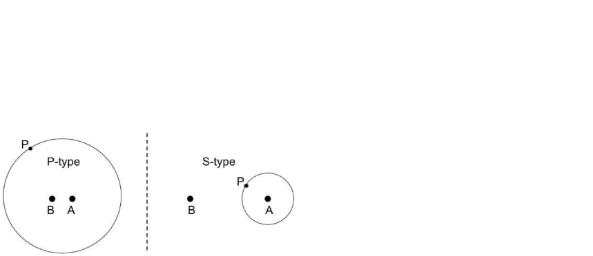
Figure 1: S-type and P-type binary-planetary systems. A and B represent the stars of the binary, and P depicts the planet.

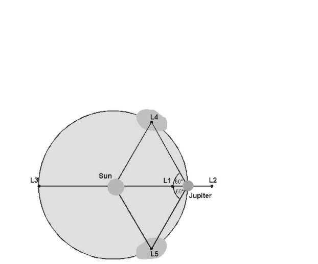
Figure 2: Schematic view of the stable region around the Lagrange points $L_{4}$ and $L_{5}$ in the restricted three body problem with the Sun and Jupiter as primary bodies

The stability of a planetary orbit in dual-star systems depends also on the type of its orbit. From a dynamical point of view, three types of motion are recognized in double-star systems (see figures 1 and 2, and Dvo84 ):

1. the S-type (or the satellite-type), where the planet moves around one stellar component,

2. the P-type (or the planet-type), where the planet surrounds both stars in a distant orbit, and

3. the L-type (or the libration-type), where the planet moves in the same orbit as the secondary (i.e., locked in a 1:1 mean motion resonance), but $60^{\circ}$ ahead or behind.

Within the framework of elliptical restricted three-body problem (ER3BP), many authors have studied the stability of planets in binaries for different types of above-mentioned planetary orbits Dvo84 ; Dvo86 ; Rab88 ; Dvo89 ; Dvo91 ; Loh93 ; Ben88a ; Ben88b ; Ben89 ; Ben93 ; Ben96 ; Ben98 ; Holman97 ; Hol99 ; Pil02 . However, because until 2003, no planet had been detected in or around a double star, the applicability of the results of these studies were only to hypothetical systems. The discovery of the first planet in a moderately close binary by Hat03 changed this trend and encouraged many researcher to revisit this problem and explore the stability of planets in binaries by considering more realistic cases (see, for instance, Pil03 ; Dvo03a ; Dvo03b ; Dvo04 ; Hag06 ; Inn97 ; Mus05 ).

In this chapter, we focus on the stability and habitability of planets in S-type orbits. As shown in Table 1, all the currently known planets in binary systems (regardless of the separation of the binary) are of this kind. We present the results of the studies of the general stability of S-type orbits and discuss their application to real binary systems, in particular the system of $\gamma$ Cephei. Since the discovery of a giant planet around the primary of this double star Hat03 , many studies have been done on the stability and habitability of this binary and the possibility of the formation of giant and Earth-like planets around its stellar components Dvo03a ; The04 ; Hag05 ; Ver06 ; Tor07 . We finish this section by briefly reviewing the stability of planets in P-type and L-type orbits.

The numerical simulations of planetary orbits presented in this section are mostly carried out within the framework of the elliptical, restricted, three-body system, where the planet is regarded as a massless object with no influence on the dynamics of the binary. To determine the character of the motion of an orbit, we either use a chaos indicator, or carry out long-term orbital integrations. As a chaos indicator, we use the fast Lyapunov indicator (FLI) as developed by Fro97 . FLI can distinguish between regular and chaotic motions in a short time, and chaotic orbits can be found very quickly because of the exponential growth of this vector in the chaotic region. For most chaotic orbits only a few number of primary revolutions is needed to determine the orbital behavior. In order to distinguish between stable and chaotic motions, we define a critical value for FLI which depends on the computation time. This method has been applied to the studies of many extrasolar planetary systems by Pil02 ; Dvo03a ; Dvo03b ; Pil03 ; Boi03 ; Erd03 ; Pil05 ; San06 .

When carrying out long-term orbital integrations, a fast and reliable characterization of the motion can be achieved by making maps of the maximum eccentricity of the orbit of the planet calculated for each integration of its orbit. The maximum eccentricity maps can be used as a useful indicator of orbital stability, especially for studies of the motion of terrestrial-size planets in the habitable zone of their host stars. Examples of such studies can be found in the works of Dvo03a ; Fun04 ; Erd04 ; Dvo04 ; Asg04 , and Pil06 .

2.1 Stability of S-type orbits

The motion of a planet in an S-type orbit is governed by the gravitational force of its host star and the perturbative effect of the binary companion. Since the latter is a function of the distance between the planet and the secondary star, the orbit of the planet will be less perturbed if this distance is large. In other words, a planet in an S-type orbit will be able to maintain its orbit for a long time if it is sufficiently close to its parent star Har77 . By numerically integrating the motion of a massless object in an S-type orbit, Rab88 (hereafter RD) and Hol99 (hereafter HW) have shown that the maximum value of the semimajor axis of a stable S-type orbit varies with the binary mass-ratio, semimajor axis, and eccentricity as,

$$\!\!\!\!\!\!\!\!\!\!\!\!\!\!\!\!\!\!\!\!\!\!\!\!{{a_{c}}/{a_{b}}}=(0.464\pm 0.006)+(-0.380\pm 0.010)\mu+(-0.631\pm 0.034){e_{b}}$$

$$\qquad+(0.586\pm 0.061)\mu{e_{b}}+(0.150\pm 0.041){e_{b}^{2}}+(-0.198\pm 0.047)\mu{e_{b}^{2}}\>.$$ (1)

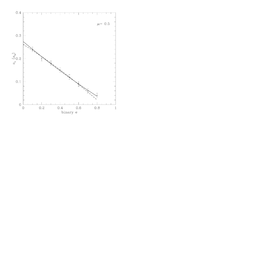
Figure 3: Graphs of the critical semimajor axis $(a_{c})$ of an S-type binary-planetary system, in units of the binary semimajor axis Hol99 . The graph on the top shows $a_{c}$ as a function of the binary eccentricity for an equal-mass binary. The graph on the bottom corresponds to the variations of the critical semimajor axis of a binary with an eccentricity of 0.5 in term of the binary’s mass-ratio. The solid and dashed line on the top panel depict the empirical formulae as reported by Hol99 and Rab88 , respectively.

In this equation, $a_{c}$, the critical semimajor axis, is the upper limit of the semimajor axis of a stable S-type orbit, $a_{b}$ and $e_{b}$ are the semimajor axis and eccentricity of the binary, and $\mu={{M_{2}}/{({M_{1}}+{M_{2}}})}$, where $M_{1}$ and $M_{2}$ are the masses of the primary and secondary stars, respectively. Figure 3 shows the variation of $a_{c}$ with the binary mass-ratio and eccentricity. As expected, S-type orbits in binaries with larger secondary stars on high eccentricities are less stable. The $\pm$ signs in equation (1) define a lower and an upper value for the critical semimajor axis which correspond to a transitional region that consists of a mix of stable and unstable orbits. Such a dynamically gray area, in which the state of a system changes from stability to instability, is known to exist in multi-body environments, and is a characteristic of any dynamical system. Similar studies have been done by Moriwaki04 and Fatuzzo06 who obtained critical semimajor axes slightly larger than given by equation (1).

It is necessary to mention that in simulations of RD and HW, the initial orbit of the planet was considered to be circular. In a series of numerical integrations, Pil02 (hereafter PLD) considered non-zero values for the initial eccentricity of the planet and by assuming the following initial conditions, they analyzed the influence of the planet’s eccentricity on its orbital stability.

For the binary, these authors assumed

• a semimajor axis of 1 AU,

• an eccentricity between 0 and 0.9 in steps of 0.1, and

• an initial starting point for the secondary star at either its periastron or apastron.

For the planet, which moves around the primary in the same plane as the orbit of the binary (i.e., coplanar orbits), they considered

• a semimajor axis between 0.1 AU and 0.9 AU,

• an initial eccentricity between 0 and 0.5 in increments of 0.1 for all binary mass-ratios, and

• a starting point with different angular positions (i.e. mean anomaly $=0^{\circ}$ or $90^{\circ}$ or $180^{\circ}$ or $270^{\circ}$),

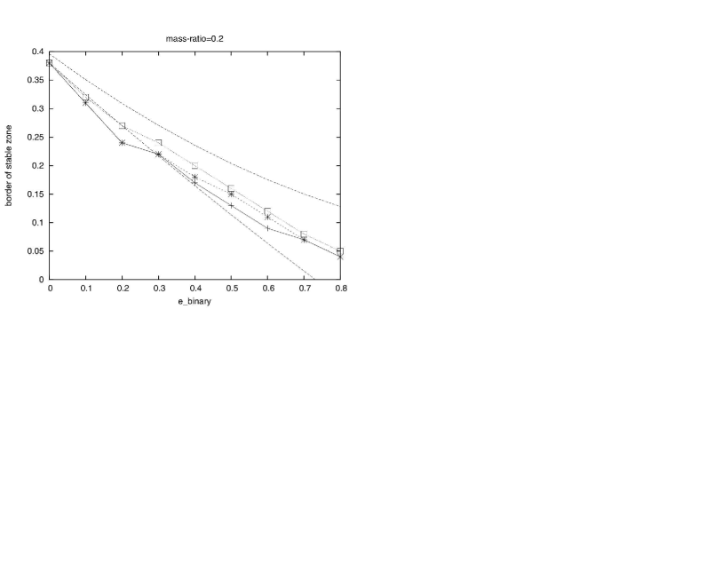
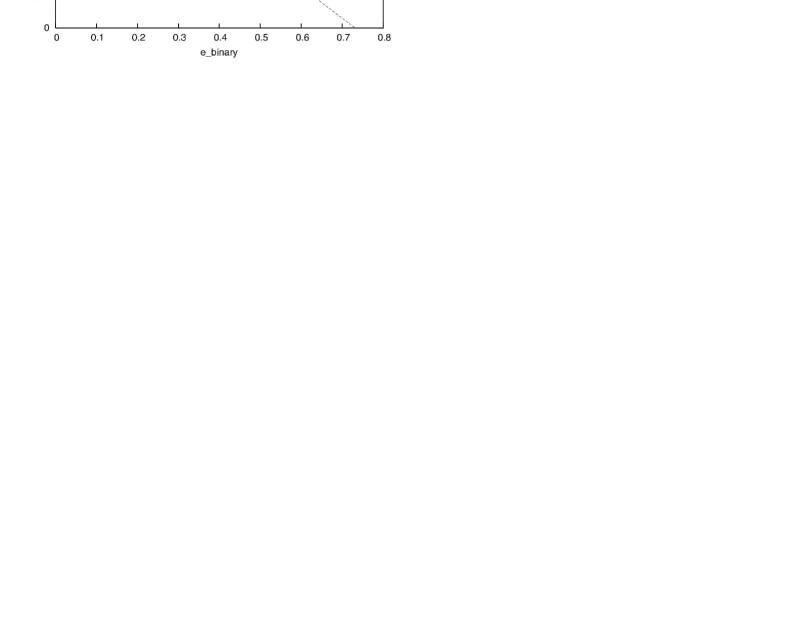
Figure 4: A comparison of the results of PLD with those of HW. The upper panel shows the results for $e_{p}=0$ (solid line with crosses) and $e_{p}=0.1$ (dashed line with stars) as obtained by PLD. The dotted line with white squares shows the results obtained by HW. The area between the two dashed lines defines the boundary of the stable zone according to equation (1). The lower panel shows the results of PLD for $e_{p}$ ranging from 0.3 to 0.9.

Figure 4 shows a comparison of the results of the three studies by RD, HW, and PLD, in a binary with a mass-ratio of $\mu=0.2$. In this figure, the value of the critical semimajor axis of the planet is shown for different values of its eccentricity and the eccentricity of the binary. The boundaries of the stability zone corresponding to HW simulations (calculated using equation 1) are shown in dotted lines. As shown in the top panel of this figure, stability zones of low-eccentricity orbits, as obtained by PLD, are in a good agreement with the results of HW. However, for planets with larger orbital eccentricities, as shown in the lower panel, the size of the stability zone decreases as the eccentricity of the planet increase. The plotted stability boundaries for such orbits fall outside the HW stable zone and are closer to the planet-hosting star. This can also be seen in Table 2, where the lesser of the values of the inner boundary of the stable region (i.e. the semimajor axis of the last stable orbit) as obtained by HW and PLD, has been recorded. These results indicate that the stability criteria presented by HW are not applicable to eccentric S-type orbits.

It is necessary to mention that as oppose to RD and HW who determined the stable zone of a planet by identifying its escaping orbits within a certain computation time, PLD used a chaos indicator to characterize the long-term behavior of the planet’s motion. Although because of the application of FLI, the computation time in PLD was much shorter than in RD and HW, their results are, however, valid for much longer times. In some cases in simulations by PLD, the application of FLI resulted in a slightly larger stable region compare to that of HW. This is due to the fact that, as oppose to the latter, in which 8 starting points were used, PLD used only 4 starting positions. Test-computations, using a different grid for the FLI-maps, and for computation times over $10^{4},10^{5}$ and $10^{6}$ periods of the binary were also carried out. However, they did not change the result significantly.

Table 2: Stable zone (in units of the binary semimajor axis) of an S-type orbit for different values of the mass-ratio and eccentricity of the binary. The given size for each $(\mu,{e_{b}})$ pair is the lesser of the values obtained by HW and PLD.

Mass-ratio $(\mu)$
$e_{b}$ 0.1 0.2 0.3 0.4 0.5 0.6 0.7 0.8 0.9 0.0 0.45 0.38 0.37 0.30 0.26 0.23 0.20 0.16 0.13 0.1 0.37 0.32 0.29 0.27 0.24 0.20 0.18 0.15 0.11 0.2 0.32 0.27 0.25 0.22 0.19 0.18 0.16 0.13 0.10 0.3 0.28 0.24 0.21 0.18 0.16 0.15 0.13 0.11 0.09 0.4 0.21 0.20 0.18 0.16 0.15 0.12 0.11 0.10 0.07 0.5 0.17 0.16 0.13 0.12 0.12 0.09 0.09 0.07 0.06 0.6 0.13 0.12 0.11 0.10 0.08 0.08 0.07 0.06 0.045 0.7 0.09 0.08 0.07 0.07 0.05 0.05 0.05 0.045 0.035 0.8 0.05 0.05 0.04 0.04 0.03 0.035 0.03 0.025 0.02

Table 3 shows the variations of the size of the stable zone in simulations of PLD in terms of the eccentricities of the binary and planet, and for different binary mass-ratios. As shown here, as the eccentricity of the binary increases, the boundary of the stable zone varies from 0.04 (for an initially eccentric motion in a binary with an eccentricity of 0.5 and mass-ratio of $\mu=0.9$) to 0.45 (for an initially circular motion in a circular binary with $\mu=0.1$). Table 3 also shows that the size of the stable region does not have a strong dependence on the eccentricity of the planet. This dependence is not, however, negligible, especially if a planet is close to the border of the chaotic motion and moves in a highly eccentric orbit. A presentation of the 3-D stability plots for different mass-ratios with a detailed discussion can be found in PLD.

Table 3: Stable zone (normalized to $a_{b}$) of an S-type orbit

Stable Zone
Mass-ratio $(\mu)$ $e_{b}$ ${e_{p}}=0$ ${e_{p}}=0.5$ 0.1 0 0.45 0.36 0.5 0.18 0.13 0.2 0 0.40 0.31 0.5 0.16 0.12 0.3 0 0.37 0.28 0.5 0.14 0.11 0.4 0 0.30 0.25 0.5 0.12 0.07 0.5 0 0.27 0.22 0.5 0.12 0.07 0.6 0 0.23 0.21 0.5 0.10 0.07 0.7 0 0.20 0.18 0.5 0.09 0.07 0.8 0 0.16 0.16 0.5 0.09 0.05 0.9 0 0.13 0.12 0.5 0.06 0.04

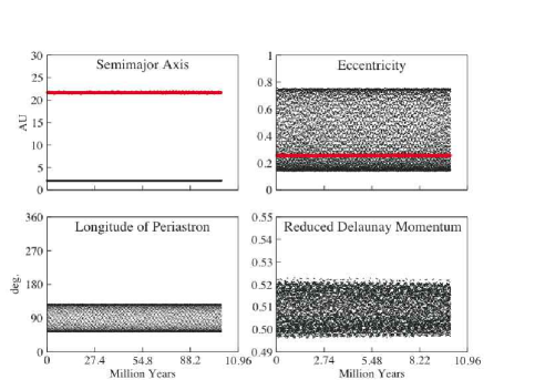
Figure 8: Graphs of the semimajor axis and eccentricity of the giant planet (black) and binary (red) of $\gamma$ Cephei (top) and its longitude of periastron and reduced Delaunay momentum (bottom) in a Kozai resonance Hagh04 ; Hagh05a . As expected, the longitude of the periastron of the giant planet oscillates around $90^{\circ}$ and its reduced Delaunay momentum is constant.

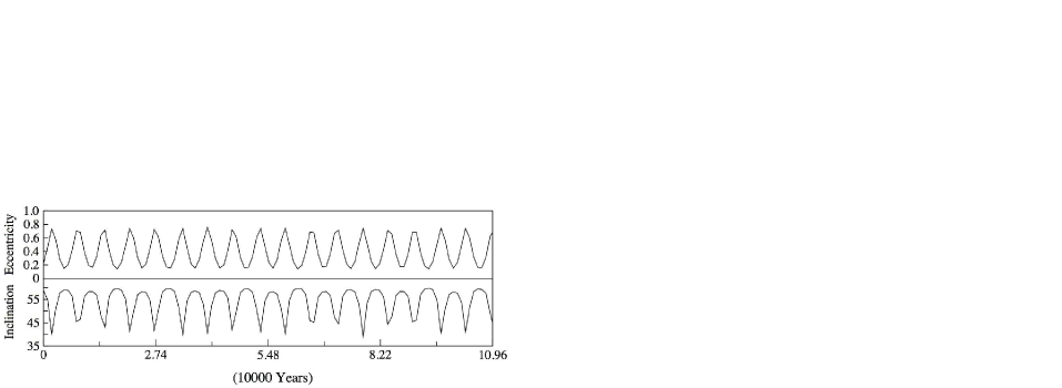
Figure 9: Graphs of the eccentricity and inclination of the giant planet of $\gamma$ Cephei in a Kozai Resonance Hagh04 ; Hagh05a . As expected, these quantities have similar periodicity and are $180^{\circ}$ out of phase.

An interesting application of the analysis of HW and PLD is to the stability of terrestrial planets and smaller objects. Since in the calculations of the critical semimajor axis by these authors, a giant planet was consider to be a test particle, given that the mass of a Jovian-type planet is approximately two orders of magnitude larger than the mass of a terrestrial-class object, the stability criteria of HW and PLD can be readily generalized to identify regions around the stars of a binary where terrestrial-class planets can have long-term stable orbits Quintana02 ; Quintana06 ; Quintana07 . This results can also be used to identify regions where smaller objects, such as asteroids, comets, and/or dust particles may reside. Although these analyses do not include non-gravitational forces, their applications to observational data has been successful and have identified dust bands, possibly due to the collision among planetesimals, in several wide S-type binaries (see figures 8 and 9 of chapter 1, and Trilling07 ).

Application to the binary $\gamma$ Cephei

Gamma Cephei is one of the most interesting double star systems that host a planet. At a distance of approximately 11 pc from the Sun, and with a semimajor axis and an eccentricity of 18.5 AU and 0.36, respectively, this system present a prime example of a moderately close binary with a planet in an S-type orbit. The primary of $\gamma$ Cephei, a 1.6 solar-mass K1 IV sub-giant Fuhr04 is host to a stellar companion, an M4 V star with a mass of 0.4 solar-masses Neu07 ; Tor07 , and a Jovian-type planet with a mass of 1.7 Jupiter-mass and an eccentricity of 0.12 at 1.95 AU Hat03 .

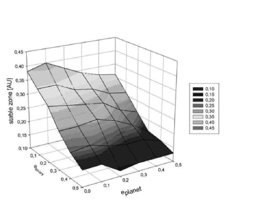
Figure 5: The stable zone of an S-type orbit in a binary with mass-ratio $\mu=0.2$ (e.g., $\gamma$ Cephei). As shown here, the extent of the stable zone is more strongly affected by the eccentricity of the binary than that of the planet Pilat04 .

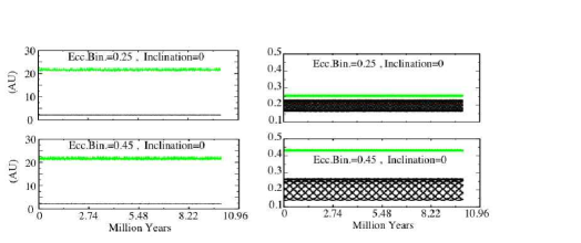
Figure 6: Graphs of the semimajor axes (left) and eccentricities (right) of the giant planet (black) and binary (green) of $\gamma$ Cephei for different values of the eccentricities of the binary Hagh04 . The mass-ratio of the binary is 0.2.

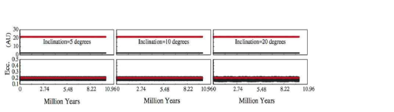
Figure 7: Graphs of the semimajor axes (top) and eccentricities (bottom) of the giant planet (black) and binary (red) of $\gamma$ Cephei. The initial eccentricity of the binary at the beginning of numerical integration and the value of its mass-ratio were equal to 0.20 Hag06 .

The mass-ratio of $\gamma$ Cephei binary is 0.2 making this system a suitable example for applying the stability analysis of S-type orbits as discussed in the previous section. An overview of the size of the stable region for the giant planet of this system is shown in figure 5 where the planet maintained its orbit for 1000 time units. As shown in this figure, the zone of stability for the giant planet extends to approximately 3.16 AU. Direct integration of the binary and the planet for different values of the binary eccentricity indicate that the orbit of the planet is stable when $0.2\leq{e_{b}}\leq 0.45$ Hag06 . Samples of the results of these integrations are shown in figure 6. Numerical integrations of the orbit of the planet for different values of its inclination with respect to the plane of the binary $(i_{p})$ show that this object is stable for inclinations less than 40^∘. Figure 7 shows the semimajor axes and orbital eccentricities of the system for ${e_{b}}=0.2$ and for $i_{p}$=5^∘, 10^∘, and 20^∘.

Numerical simulations also indicated the possibility of a Kozai resonance in the $\gamma$ Cephei system. Kozai resonance has been studied in binary-planetary systems by several authors Hagh04 ; Hagh05a ; Ver06 ; Takeda06 ; Malmberg07 ; Takeda08 ; Saleh09 . As demonstrated by Kozai62 , in a three-body system with two massive bodies and a small object, such as an S-type binary-planetary system, the orbital eccentricity of the planet can reach high values at large inclinations due to the exchange of angular momentum between the planet and the secondary star. In such cases, the longitude of the periastron of the planet, $\omega_{p}$, librates around a fix value. Figure 8 shows this for the giant planet of $\gamma$ Cephei. As shown here, $\omega_{p}$ librates around 90^∘ Hagh04 ; Hagh05a . The inclination of the planet of $\gamma$ Cephei, when in a Kozai resonance, is related to its longitude of periastron and orbital eccentricity $(e_{p})$ as Inn97

$${\sin^{2}}{\omega_{p}}=\,0.4\,{\csc^{2}}{i_{p}},$$ (2)

and

$${(e_{p}^{2})_{\rm max}}={1\over 6}\,\Bigl{[}1-5\cos(2{i_{p}})\Bigr{]}.$$ (3)

Equation (2) indicates that the Kozai resonance may occur if the orbital inclination of the small body is larger than 39.23^∘. For instance, as shown by Hagh04 ; Hagh05a , in the system of $\gamma$ Cephei, Kozai resonance occurs at ${i_{p}}={60^{\circ}}$. For the minimum value of ${i_{p}}$, the maximum value of the planet’s orbital eccentricity is reached and, as given by equation (3), is equal to 0.764. Figures 8 and 9 show that $e_{p}$ stays below this limiting value at all times.

Application to binaries Gliese 86 and HD41004

The application of the stability analysis of section 2.1 to the planet of the binary Gliese 86 indicates that the orbit of this planet is stable. This is not surprising since with a semimajor axis of 0.11 AU, this planet is close enough to the primary star to be immune from the perturbation of the other stellar companion.

In the case of HD41004, the application of the stability analysis of section 2.1 is not straightforward; the orbital parameters of the planet in this binary has not been uniquely determined. The value of the semimajor axis of this planet varies between 1.31 AU and 1.7 AU, and its orbital eccentricity seems to be quite high (between 0.39 and 0.74) Zucker04 . Since the eccentricity of the binary HD41004 is unknown, to determine the stable zone of this system, simulations were carried out for different sets of orbital parameters as a function of the binary eccentricity. The results indicate that the stability of the planet is strongly correlated with its orbital eccentricity and the eccentricity of the binary. Simulations show that in all cases, in order to obtain stability, binary eccentricity has to be smaller than 0.6. For high values of the planet’s eccentricity (e.g., 0.74), the value of the binary eccentricity has to become even smaller (less than 0.15) to ensure that the orbit of the planet will stay stable.

2.2 Stability of P-type Orbits

Although, no circumbinary planet has yet been discovered, stability of P-type orbits has been a subject of research for many years Ziglin75 ; Szebehely81 ; Dvo84 ; Dvo86 ; Dvo89 ; Kubala93 ; Hol99 ; Broucke01 ; Pil03 ; Mus05 . In general, a planet in a P-type orbit is stable if its distance from the binary is so large that the perturbations of the binary stars cannot disturb its motion. Such a stable planet cannot, however, orbit the binary too far from its center of mass since galactic perturbations and the effects of passing stars may make the orbit of the planet unstable. As shown by Dvo84 , for circular binaries, this distance is approximately twice the separation of the binary, and for eccentric binaries (with eccentricities up to 0.7) the stable region extends to four time the binary separation. Subsequent studies by Dvo86 ; Dvo89 and Hol99 have shown that Dvorak’s 1984 results can be formulated by introducing a critical semimajor axis below which the orbit of the planet will be unstable;

$$\!\!\!\!\!\!\!\!\!\!\!\!\!\!\!\!\!\!\!\!\!\!\!\!\!\!{a_{c}}/{a_{b}}=(1.60\pm 0.04)+(5.10\pm 0.05){e_{b}}+(4.12\pm 0.09)\mu$$

$$\qquad\qquad+(-2.22\pm 0.11){e_{b}^{2}}+(-4.27\pm 0.17){e_{b}}\mu+(-5.09\pm 0.11){\mu^{2}}$$

$$\!\!\!\!\!\!\!\!\!\!\!\!\!\!\!\!\!\!\!\!\!\!\!\!\!\!\!\!\!\!\!\!\!\!\!\!\!\!\!\!\!\!\!\!\!\!\!\!\!\!\!\!\!\!\!\!\!\!\!\!\!\!\!\!\!\!\!\!\!\!\!\!\!\!\!+(4.61\pm 0.36){e_{b}^{2}}{\mu^{2}}\>.$$ (4)

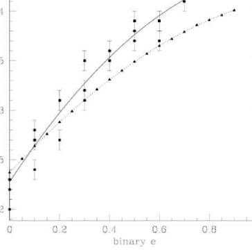
Figure 10: Critical semimajor axis as a function of the binary eccentricity in a P-type system. The squares correspond to the result of stability simulations by Hol99 and the triangles represent those of Dvo89 . The solid line corresponds to equation (4). As indicated by Hol99 , the figure shows that at outer regions, the stability of the system fades away.

Figure 10 shows the value of $a_{c}$ for different values of the binary eccentricity. Similar to S-type orbits, the $\pm$ signs in equation (4) define a lower and an upper value for the critical semimajor axis $a_{c}$, and set a transitional region that consists of a mix of stable and unstable orbits. We refer the reader to Hol99 ; Pil03 and Pil06a for more details. Using this stability criteria in analysis of their observational data, Trilling07 have been able to detect circumbinary dust bands, possibly resulted from the collision of planetesimal, around several close binary stars (Chapter 1, figures 8 and 9).

A dynamically interesting feature of a circumbinary stable region is the appearance of islands of instability. As shown by Hol99 , islands of instability may develop beyond the inner boundary of the mixed zone, which correspond to the locations of $(n:1)$ mean-motion resonances. The appearance of these unstable regions have been reported by several authors under various circumstances Henon70 ; Dvo84 ; Rab88 ; Dvo89 . Extensive numerical simulations would be necessary to determine how the overlapping of these resonances would affect the stability of P-type binary-planetary orbits.

2.3 Stability of L-Type Orbits

The L-type orbit, in which an object librates around one of the binary’s Lagrangian triangular points (figure 2), may not be entirely relevant to planetary motions in double star systems. The reason is that such an orbital configuration requires ${M_{2}}/{({M_{1}}+{M_{2}})}\leq 1/26$, which is better fulfilled in systems consisting of a star and a giant planet. Recent simulation by Hagh08 have shown that in systems with a close-in giant planet, L-type planetary orbits with low eccentricities can be stable for long times. We refer the reader to section 3.2 and the paper by Pil03 for more details on the stability of these orbits.

3 Terrestrial Planets in Binaries

In the previous section, a general analysis of the dynamics of a planet in a binary star system was presented. However, within the context of habitability, the interest falls on the motion and long-term stability of Earth-like planets. It would be interesting to extend studies of the habitability, similar to those by Jon01 and Men03 , to binary star system, in particular those in which a giant planet already exists, and analyze the dynamics of fictitious Earth-like planets in such complex environments. In this section, we focus on this issue.

In general, four different types of orbits are possible for a terrestrial planet in a binary system that hosts a giant planet:

• TP-i : the terrestrial planet is inside the orbit of the giant planet,

• TP-o : the terrestrial planet is outside the orbit of the giant planet,

• TP-t : the terrestrial planet is a Trojan of the primary (or secondary) or the giant planet,

• TP-s : the terrestrial planet is a satellite of the giant planet.

In principle, the study of the stability of these orbits requires the analysis of the dynamics of a complicated N-body system consisting of two stars, a giant planet, and a terrestrial-class object. Except for a few special cases, the complexities of these systems do not allow for an analytical treatment of their dynamics, and require extensive numerical integrations. Those special cases are:

• binaries with semimajor axes larger then 100 AU in which the secondary star is so far away from the primary (the planet-hosting star) that its perturbative effect can be neglected Jim02 ,

• binaries in which the giant planet has an orbit with a very small eccentricity (almost circular),

• binaries in which, compared to the masses of the other bodies, the mass of the terrestrial planet is negligible. In these systems, within the framework of ER3BP, one can define curves of zero-velocity, the barriers of the motion of the fictitious terrestrial planet, using the Jacobi constant Dvo03 .

When numerically studying the dynamics of a terrestrial planet in a binary-planetary system, integrations have to be carried out for a vast parameter-space. These parameters include the semimajor axes, eccentricities, and inclinations of the binary and the two planets, the mass-ratio of the binary, and the ratio of the mass of the giant planet to that of its host star. The angular variables of the orbits of the two planets also add to these parameters. Although such a large parameter-space makes the numerical analysis of the dynamics of the system complicated, numerical integrations are routinely carried out to study the dynamics of terrestrial planets in binary-planetary systems. The reason is that such numerical computations allows for the investigation of the stability of many terrestrial planets and for a grid of their initial conditions in one or only a few simulations. Given the small size of these objects compared to that of a giant planet (e.g., 1/300 in case of Earth and Jupiter), to the zeroth order of approximations, the effect of a terrestrial planet on the motion of a giant planet can be ignored, and the terrestrial planet can be considered as a test particle. This simplification makes it possible to study the stability of thousands of possible orbits of a terrestrial-class body in one integration. Several studies of the dynamical evolution of a terrestrial planet in a binary system have used this simplification and have shown that the final results are quite similar to the results of the numerical integrations of an actual four-body system Dvo04 ; Erd05 .

In the rest of this section, we present the results of the studies of the dynamics of a terrestrial planet, focusing primarily on TP-i and TP-o orbits. Since no extrasolar terrestrial planet has yet been discovered, the only possible approach for a detailed dynamical analysis of the orbit of such an object in a binary system is to consider a specific extrasolar planetary system in a double star, and study the dynamics of a fictitious terrestrial planet for different values of its orbital elements, and those of the binary and its giant planets. As an example, we will consider the binary-planetary system of $\gamma$ Cephei. For the orbital elements of this system, we use the values given by Hag06 and Neu07 .

3.1 Stability of TP-i and TP-o Orbits

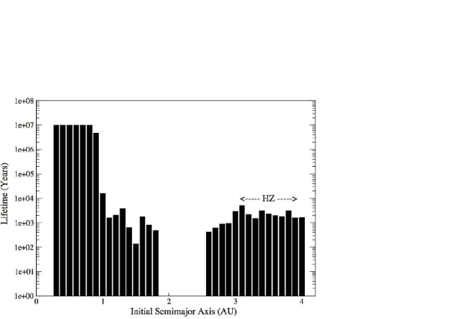
Figure 11: Graph of the lifetime of an Earth-size object in a circular orbit around the primary of $\gamma$ Cephei. The habitable zone of the primary has been indicated by HZ. No planet was placed in the region between the aphelion and perihelion distances of the giant planet of the system. As shown here, only Earth-size planets close to the primary star maintain their orbits for long times Hag06 .

A study of the dynamics of a full four-body system consisting of a terrestrial planet in a TP-i or TP-o orbit in $\gamma$ Cephei indicates that the orbit of this planet can only be stable in close neighborhood of the primary star and outside the influence zone of the giant planet (figure 11, Hag06 ). Integrations also show that, while the habitable zone of $\gamma$ Cephei is unstable Hag06 ; Dvo03a , it is possible for an Earth-like planet to have a stable TP-i orbit in a region between 0.3 AU and 0.8 AU from the primary star, and when its orbit is coplanar with that of the giant planet with an inclination less than $10^{\circ}$. In the region outside the orbit of the giant planet, i.e. when the terrestrial planet is in a TP-o orbit, the perturbations from the giant planet and the secondary star affect the stability of this object. For instance, for the values of the binary eccentricity equal to ${e_{b}}$=0.25, 0.35, and 0.45, the periastron of the secondary star will be as close as 13.9 AU, 12.0 AU, and 10.2 AU, respectively. At these distances, the secondary will have strong effects on the stability of the orbit of a terrestrial planet with a semimajor axis between 2.5 AU and 5.8 AU. Simulations show that no orbit survives in this region longer than approximately $10^{5}$ years. For TP-o orbits inside 2.5 AU, the perturbation of the giant planet is the main factor in the instability of the orbit of the terrestrial planet.

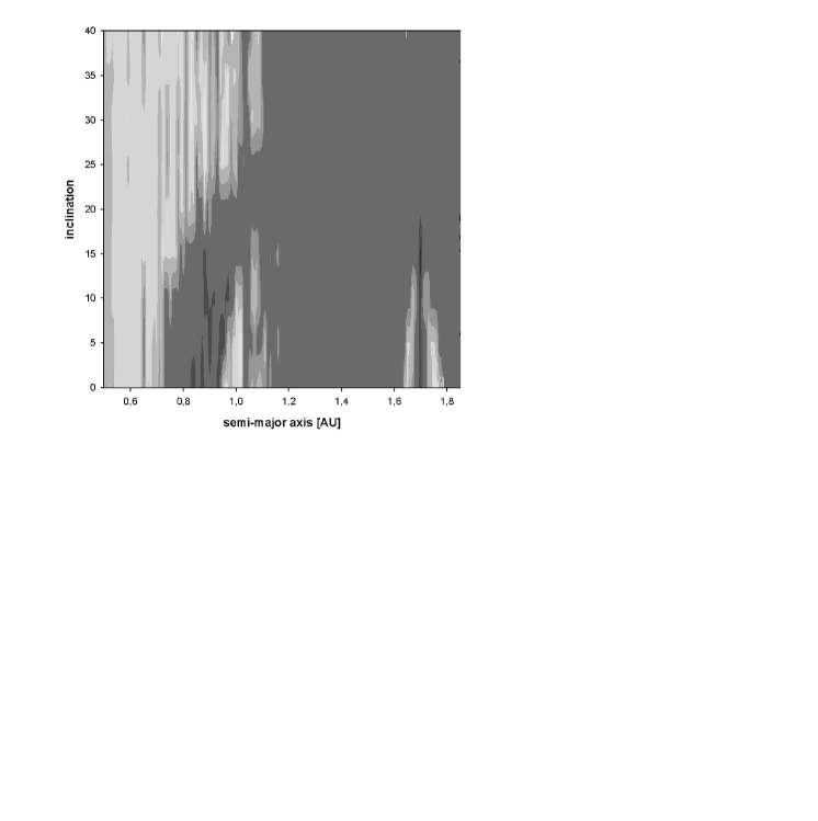
Figure 12: Stability maps for a fictitious terrestrial planet in the $\gamma$ Cephei system. Dark regions represent chaotic zones and gray regions correspond to stability. The upper graph shows the stability of a terrestrial planet in a restricted four-body problem (R4BP) [i.e. $\gamma$ Cephei binary + detected planet + fictitious (massless) planet]. The lower panel shows the results in a restricted three-body problem (R3BP) [i.e. primary + detected planet + fictitious planet] Pilat04 .

To study the effect of orbital inclination on the stability of a terrestrial planet in $\gamma$ Cephei, the region between the host-star and the giant planet of this system was examined for different values of the inclination of a fictitious terrestrial-size object, with and without the secondary star Pilat04 . Figure 12 shows the results. While dynamical models using two massive bodies (i.e., primary star and the giant planet) show a vast region of stability for a massless terrestrial planet (gray area in the lower panel of figure 12), models with three massive bodies (i.e., primary, secondary, and the giant planet), show a decrease in the stable region (see upper panel of figure 12). They also show an arc-like chaotic path with an island of stability around 1 AU, which corresponds to the 3:1 mean motion resonance with the giant planet.

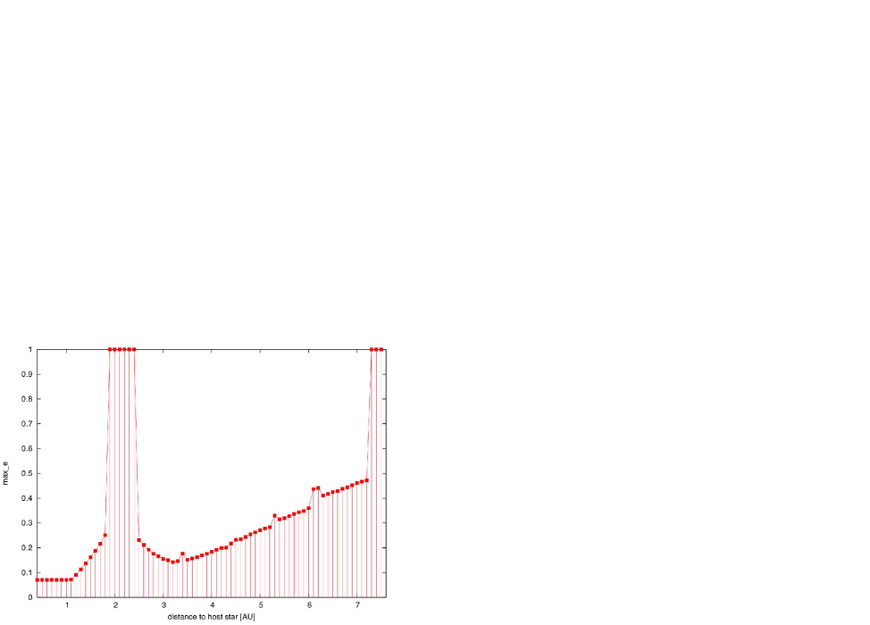
Figure 13: Graph of the eccentricity of a massless terrestrial planet in a retrograde orbit in the $\gamma$ Cephei system. Integrations were carried out for 1 Myr within a restricted four-body system. The three peaks at 3.4 AU, 5.3 AU, and 6.1 AU correspond to 2:1, 4:1, and 5:1 mean-motion resonances between the terrestrial and the giant planets.

The instability of the orbit of a terrestrial planet in $\gamma$ Cephei system (in particular in its habitable zone) has been studied only for prograde orbits. Recently in an article by Gay08 , the authors investigated the stability of retrograde orbits in extrasolar planetary systems with multiple planets and showed that in systems were prograde orbits are unstable (e.g., HD 73256), retrograde orbits may survive for long times. The stability of retrograde orbits in planetary systems has been known for many years Har72 ; Har75 ; Har77 ; Don94 . Such long-term stable orbits have also been observed among Jupiter’s retrograde irregular satellites Jewitt07 . To investigate whether retrograde TP-i and TP-o orbits can survive in a binary-planetary system, the motion of a massless terrestrial planet in these orbits was simulated for 1 Myr in the binary of $\gamma$ Cephei. Figure 13 shows the results. From this figure one can see that for semimajor axes smaller than 1.8 AU, a TP-i orbit is stable. However, at close distances to the giant planet, this orbit suffers from strong perturbations from this object and becomes unstable (straight long lines around 2 AU where the eccentricity of terrestrial planet reaches unity). Figure 13 also shows that for a TP-o orbit, a stability region exists for initial semimajor axes ranging from 2.5 AU to 7.2 AU, with the minimum perturbation received at the semimajor axis of 3.2 AU. Beyond 7.2 AU, terrestrial planet becomes unstable due to the perturbation from the secondary star. The three small peaks in the stable region of figure 13 correspond to mean-motion resonances between the terrestrial planet and the giant planet. A comparison between this figure and figure 11, in which the lifetime of a terrestrial planet in a prograde circular orbit is shown, clearly indicates that $\gamma$ Cephei has a large stable region for retrograde orbits, in particular in the habitable zone of its primary star.

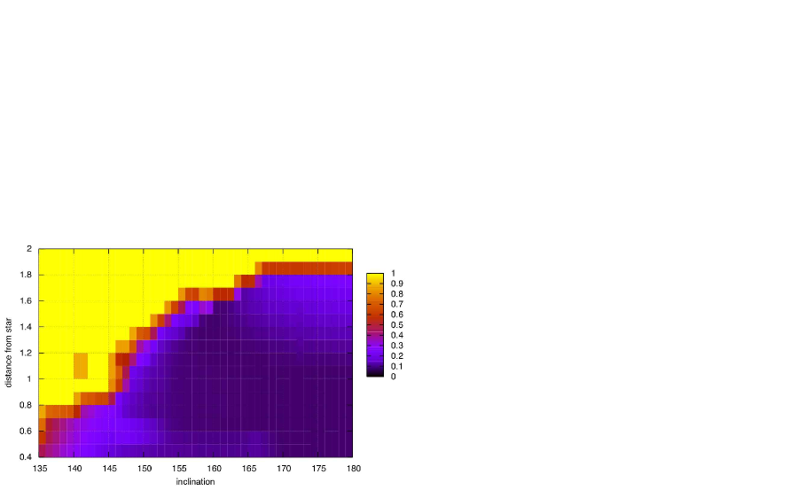
Figure 14: Stability diagram for a retrograde TP-i orbit for different values of the orbital inclination. The binary eccentricity is 0.35. Stability in shown in blue whereas yellow corresponds to chaotic orbits.

Figure 14 shows the results of the integrations of a terrestrial planet in a retrograde TP-i orbit in the $\gamma$ Cephei system, in terms of the initial orbital inclination of this object. The initial semimajor axis of the terrestrial planet was varied between 0.4 AU and 2.0 AU, and its initial orbital inclination was chosen to be between $135^{\circ}$ and $180^{\circ}$. The eccentricity of the binary was $e_{b}=0.35$. As shown in this figure, the upper stability limit for a terrestrial planet in retrograde orbits is 1.8 AU corresponding the inclinations between $165^{\circ}$ and $180^{\circ}$, and the lower limit is 0.8 AU for an inclination of $145^{\circ}$. For more inclined orbits of a fictitious terrestrial planet, this lower limit drops to 0.4 AU. Simulations for different values of the binary eccentricity indicate that the direct effect of the binary orbit on the stability of a terrestrial planet in a retrograde TP-i orbit is negligible, and it only affects the eccentricity of the orbit of the giant planet (${\delta e}_{GP}=0.08,0.1,0.11$ for $e_{b}=0.25,0.35,0.45$, respectively). It is the latter that affects the orbit of the fictitious planet in a TP-i orbit.

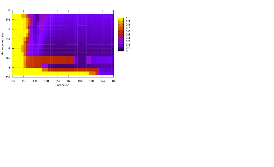
Figure 15: Stability diagram for a retrograde TP-o orbit for different values of the orbital inclination. The binary eccentricity is 0.25, 0.35, and 0.45 from top to bottom. Stability in shown in blue whereas yellow corresponds to chaotic orbits. As shown here, instability extends to large distances as the binary eccentricity increases.

The situation is different for a retrograde TP-o orbit. As shown in figure 15, although the effect of the 2:1 resonance with the giant planet at 3.1-3.6 AU makes the orbit of a retrograde terrestrial planet unstable, large stable regions, especially for lower values of the binary eccentricity, exist beyond this region and for different values of the initial inclination of the orbit of the terrestrial planet. For instance, for $e_{b}=0.25$, the region of stability extends from 3.5 AU to 5.8 AU for the values of the inclinations ranging from $145^{\circ}$ to $180^{\circ}$. At the 2:1 mean-motion resonance also a stable region exists for inclinations between $160^{\circ}$ and $180^{\circ}$, when the eccentricity of the terrestrial planet is smaller than 0.2. In the case of a binary with $e_{b}=0.35$ (figure 15, middle graph), the unstable region corresponding to the 2:1 resonance extends to higher inclinations. For the values of the eccentricity of the binary larger than 0.45, instability extends to almost all inclinations.

3.2 Stability of TP-t Orbits

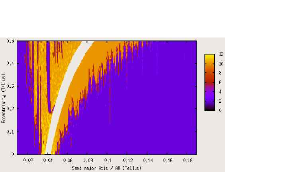
Figure 16: Graph of the stability of an Earth-sized planet in a system consisting of a Sun-like star and a transiting Jupiter-mass object in a 3 days orbit. Blue shows stability whereas red corresponds to chaos. An island of stability corresponding to the 1:1 mean-motion resonance is shown Hagh08 ; Capen09 .

An interesting case of a stable orbit is when the terrestrial planet is in a Lagrange equilibrium point either at an angular separation of $60^{\circ}$ ahead of a giant planet or behind it (figure 2). In the simplified dynamical model of the restricted (circular and elliptic) three-body system, many investigations exist concerning the stability of such a planet in terms of the mass-ratio of the planet-hosting star and its giant planet Rab61 , and the eccentricity of the giant planet’s orbit Dep70 . Within the context of extrasolar planetary systems, stability of the orbit of a terrestrial planet in a Lagrangian point has been studied by Lau02 ; Men03 ; San03 ; Erd04 ; Sch05b ; Sch07a ; Sch07b ; Sch09 . Recent simulations by Hagh08 and Capen09 show that terrestrial planets as Trojans of giant planets can also exist in systems where the giant planet transits its host star. Figure 16 shows an example of such systems. In this figure, a solar-type star is host to a Jupiter-size transiting planet in a 3-day circular orbit. The graph shows the stability of an Earth-size object for different values of its semimajor axis and orbital eccentricity. As shown here, a terrestrial planet in a 1:1 resonance with the giant planet can maintain a stable orbit for eccentricities ranging from 0.2 to 0.5.

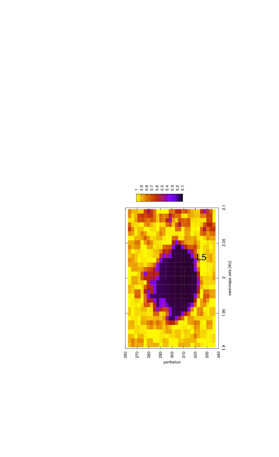
Figure 17: Stability diagram for a TP-t orbit for the region around the Lagrange points $L_{4}$ and $L_{5}$ of the giant planet in the $\gamma$ Cephei system. The angular distance to the Lagrange point are shown on the horizontal axes and the distance in AU is in the direction of the line connecting the host-star to the Lagrange point. The dark region shows the stable region.

To study the stability of TP-t orbits in the $\gamma$ Cephei system, the orbit of a terrestrial planet was integrated in a Lagrangian point of the giant planet and in a general four-body system. Because as shown by Sch07a , in order for a small body to have a stable Trojan orbit in an elliptical, restricted, three-body system, the orbital eccentricity of the giant planet cannot exceed 0.3, the eccentricity of the giant planet of $\gamma$ Cephei was set to this value. Figure 17 shows the results. As shown here, a region of stability exists for a Trojan terrestrial planet around the giant planet. Small variations in the orbital eccentricity of the giant planet, which are due to the perturbation of the secondary companion, cause the apparent asymmetry in the location of the stable orbits around the two Lagrangian points. These regions contain very stable orbits with eccentricities smaller than 0.2. The extension of semimajor axis associated with this asymmetry is small (only 2.5%). A transition from an eccentricity of 0.35 for the orbits on the edge of the stable zone, to 0.5 for orbits in the unstable region are also shown.

4 Habitable Planet Formation in Binaries

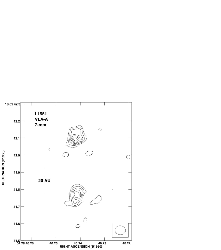
Figure 18: Interferometric observation of the binary system L1551 Rodriguez98 . Two compact sources are evident in the map. The separation of the binary is 45 AU and the disk around each core extends to approximately 10 AU. The mass of each disk is approximately 0.06 solar-masses.

As seen in previous chapters, planet formation in close and moderately close binary star systems is an active topic of research. Whether models of giant and terrestrial planet formation around single stars can be extended to binary systems depends strongly on the orbital elements of the binary, its mass-ratio, and the types of its stars. While the detection of systems such as L1551 (figure 18) implies that planet formation in binaries may proceed in the same fashion as around single stars, simulations such as those by Hep78 ; Artymowicz94 ; Whitmire98 and Pichardo05 indicate that a stellar component in an eccentric orbit can considerably affect planet formation by

• increasing the relative velocities of planetesimals, which may cause their collisions to result in breakage and fragmentation,

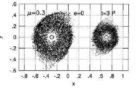
Figure 19: Disk Truncation in and around binary systems Artymowicz94 . The top graphs show circumstellar disk in a binary with a mass-ratio of 0.3. Note the disk truncation when the eccentricity of the binary is increased from 0 to 0.3. The bottom graphs show similar effect in a circumbinary disk. The mass-ratio is 0.3 and the binary eccentricity is 0.1. The numbers inside each graph represent the time in units of the binary period. The axes are in units of the binary semimajor axis.

• truncating the circumprimary disk of embryos to smaller radii, which causes the removal of material that may be used in the formation of terrestrial planets (figure 19), and

• destabilizing the regions where the building blocks of these objects may exist.

Prior to the detection of planets in binary stars, studies of planet formation in these systems were limited to only some specific or hypothetical cases. For instance, Hep74 ; Hep78 ; Drob78 ; Diakov80 ; Whitmire98 ; Kortenkamp01 studied planet formation in binaries where the system consisted of Sun and Jupiter, and the focus was on the effect of Jupiter on the formation of inner planets of our solar system. Whitmire98 studied planet formation in binaries, in particular those resembling some of extrasolar planets, in which the secondary star has a mass in the brown dwarf regime. Barbieri02 ; Quintana02 ; Lissauer04 also studied the late stage of terrestrial planet formation (i.e., growth of planetary embryos to terrestrial-size objects) in the $\alpha$ Centauri system.

The detection of the giant planet of $\gamma$ Cephei changed this trend. By providing a real example of a planetary system in a binary star, this discovery made theorist take a deeper look at the models of planet formation and focus their efforts on explaining how this planet was formed and whether such systems could harbor smaller planetary objects. The results of their works, however, have made the matter quite complicated. For instance, while simulations as those presented in chapter 10 by Quintana & Lissauer imply that the late stage of terrestrial planet formation may proceed successfully in binary star systems and result in the formation of terrestrial-class objects, simulations of earlier stages have not been able to model the accretion of planetesimals to planetary embryos. On the other hand, as indicated by Marzari and co-authors in chapter 7, despite the destructive role of the binary companion, i.e., increasing the relative velocities of planetesimals, which causes their collisions to result in erosion, growth of these objects to larger sizes may still be efficient as the effect of the binary companion can be counterbalanced by dissipative forces such as gas-drag and dynamical friction. As shown by these authors, for planetesimals of comparable sizes, the combined effect of gas-drag and the gravitational force of the secondary star may result in the alignment of the periastra of small objects and increase the efficiency of their accretion by reducing their relative velocities Marzari97 ; Marzari00 . However, the efficiency of this mechanism depends on the size of the planetesimals, the eccentricity of the planetesimals disk, and the orbital elements of the binary system. As shown by Paardekooper08 , depending on the perturbation of the secondary star, the eccentricity of the disk may reach a limiting value below which the encounter velocities of planetesimals are within a factor 2 of their corresponding values in a circular disk, and above that, the encounter velocities become so high that planetesimal accretion is inhibited. The application of these simulations to the $\alpha$ Centauri system has shown that the growth of planetesimals to planetary embryos may be impossible within 0.5 AU of the primary star of this system Thebault08 . However, simulations by Thebault09 and Marzari09 indicate that this process can be efficient around $\alpha$ Centauri B, and planetary embryos can form within the terrestrial/habitable region of this star. Similar results have been obtained by Xie08 ; Xie09 when numerically integrating a slightly inclined disk of planetesimals around the primary of $\gamma$ Cephei. As shown by these authors, the gas-drag causes the sorting of inclined planetesimals according to their sizes, and increases the efficiency of their accretion by decreasing their relative velocities. For larger values of planetesimals inclinations, accretion is more efficient in wide (e.g., $>70$ AU) binaries Marzari09 .

As one can notice, a common starting point in all these simulations is after km-sized object or larger bodies have already formed. The reason is that among the four stages of planet formation, that is,

• coagulation of dust particles and their growth to centimeter-sized objects,

• growth of centimeter-sized particles to kilometer-sized bodies (planetesimals),

• formation of Moon- to Mars-sized protoplanets (also known as planetary embryos) through the collision and accretion of planetesimals, and

• collisional growth of planetary embryos to terrestrial-sized objects,

the last two can be more readily studied in a system of double stars. At these stages, the dominant force in driving the dynamics of objects is their mutual interactions through their gravitational forces, and the simulations can be done using N-body integrations. In chapter 10 of this volume, Quintana & Lissauer have presented the results of a series of such simulations, and investigated terrestrial planet formation in binary systems such as $\alpha$ Centauri. Given that the late stage of terrestrial planet formation is a slow process, which may take a few hundred million years, it is possible that during the first few million years of this process, giant planets are also formed at large distances from the planet-hosting star. Similar to terrestrial planet formation in our solar system, these objects will play a vital role in the formation, distribution, and water-content of terrestrial-class objects in binary systems. Within the context of habitable planet formation, this implies that the formation of terrestrial planets has to be simulated while the effects of the secondary and the giant planet(s) of the system are also taken into account.

4.1 Habitable Zone

Life, as we know it, requires liquid water. A potentially habitable planet has to be able to maintain liquid water on its surface and in its atmosphere. The capability of a planet in maintaining water depends on many factors such as its size, interior dynamics, atmospheric circulation, and orbital parameters (semimajor axis and orbital eccentricity). It also depends on the brightness of the central star at the location of the planet. These properties, although at the surface unrelated, have strong intrinsic correlations, and combined with the luminosity of the star, determine the system’s habitable zone. For instance, planet’s interior dynamics and atmospheric circulation generate a CO₂ cycle, which subsequently results in greenhouse effect. The latter helps the planet to maintain a uniform temperature. This process can, however, be disrupted if the planet is too close or too far from the central star. In other words, the distance of the planet from the central star must be such that the amount of the radiation received by the planet allow liquid water to exist on its surface and in its atmosphere. The orbital elements of the planet, on the other hand, have to ensure that this object will maintain a stable orbit at all times.

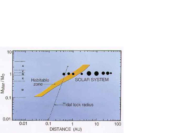
Figure 20: Habitable zone Kasting93 .

The width of a habitable zone and the location of its inner and outer boundaries vary with the luminosity of the central star and the planet’s atmospheric circulation models Men03 ; Jones05 ; Jones06 . Conservatively, the inner edge of a habitable zone can be considered as the distance closer than which water on the surface of the planet evaporates due to a runaway greenhouse effect. In the same manner, the outer edge of the habitable zone is placed at a distance where, in the absence of CO₂ clouds, runaway glaciation will freeze the water and creates permanent ice on the surface of the planet. Using these definitions of the inner and outer boundaries of a habitable zone, Kasting93 have shown that a conservative range for the habitable zone of the Sun would be between 0.95 AU and 1.15 AU from this star (figure 20). As noted by Jones05 , however, the outer edge of this region may extend to farther distances Forget97 ; Williams97 ; Mischna00 close to 4 AU.

Since the notion of habitability is based on life on Earth, one can calculate the boundaries of the habitable zone of a star by comparing its luminosity with that of the Sun. For a star with a surface temperature $T$ and radius $R$, the luminosity $L$ and its brightness $F(r)$ at a distance $r$ are given by

$$F(r)={1\over{4\pi}}L(R,T){r^{-2}}=\sigma{T^{4}}{R^{2}}{r^{-2}}\,,$$ (5)

where $\sigma$ is the Boltzmann constant. Using equation (5) and the fact that Earth is in the habitable zone of the Sun, the radial distances of the inner and outer edges of the habitable zone of a star can be obtained from

$$r\,=\,{\Bigl{(}{{T}\over{T_{\rm S}}}\Bigr{)}^{2}}\,{\Bigl{(}{{R}\over{R_{\rm S}}}\Bigr{)}}\,{r_{E}}.$$ (6)

In this equation, $T_{\rm S}$ and $R_{\rm S}$ are the surface temperature and radius of the Sun, respectively, and $r_{E}$ represents the distance of Earth from the Sun (i.e., the inner and outer edges of Sun’s habitable zone). Using equation (6), the habitable zone of a star can be defined as a region where an Earth-like planet receives the same amount of radiation as Earth receives from the Sun, so that it can develop and maintain similar habitable conditions as those on Earth.

4.2 Formation of Habitable Planets in S-Type Binaries

As mentioned earlier, a potentially habitable planet has to have a stable orbit in the habitable zone of its host star. Simulations of the stability of an Earth-size planet in the $\gamma$ Cephei system (figure 11) indicate that in an S-type binary, the region of the stability of this object is close to the primary, where the terrestrial planet is safe from the perturbations of the giant planet and the secondary star. This implies that in order for the primary to host a habitable planet, its habitable zone has to also fall within those distances where the orbit of an Earth-like planet is stable. Within this framework, Hagh07 considered a binary star with a giant planet in an S-type orbit and simulated the late stage of the formation of Earth-like planets in the habitable zone of its primary star. In their simulations, these authors assumed that

• the primary star is Sun-like with a habitable zone extending from 0.9 AU to 1.5 AU Kasting93 ,

• a Jupiter-mass planet has already formed in a circular orbit at 5 AU from the primary star,

• the collisional growth of planetesimals has been efficient and has formed a disk of planetary embryos (e.g., via oligarchic growth Ida98 ),

• the water-mass fraction of embryos is similar to the current distribution of water in primitive asteroids of the asteroid belt Abe00 . That is, embryos inside 2 AU are dry, the ones between 2 to 2.5 AU contain 1% water, and those beyond 2.5 AU have a water-mass fraction of 5% Raymond04 ; Raymond05a ; Raymond05b ; Raymond06a ; Raymond06b , and

• the initial iron content for each embryo is obtained by interpolating between the values of the iron contents of the terrestrial planets Lodders98 ; Raymond05a ; Raymond05b , with a dummy value of 40% in place of Mercury because of its anomalously high iron content.

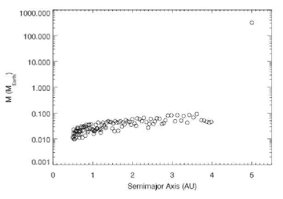
Figure 21: Radial distribution of original protoplanetary objects Hagh07 .

The model of Hagh07 also includes a circumprimary disk of 115 Moon-to Mars-sized bodies, with masses ranging from 0.01 to 0.1 Earth-masses. These objects were randomly distributed between 0.5 AU and 4 AU by 3 to 6 mutual Hill radii. The masses of embryos were increased with their semimajor axes $(a)$ and the number of their mutual Hill radii $(\Delta)$ as ${a^{3/4}}{\Delta^{3/2}}$ Raymond04 . The surface density of the disk was assumed to vary as $r^{-1.5}$, where $r$ is the radial distance from the primary star, and was normalized to a density of 8.2 g/cm² at 1 AU. Figure 21 shows the graph of one of such disks where the total mass is approximately 4 Earth-masses.

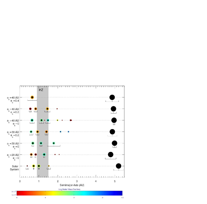
Figure 22: Results of the simulations of habitable planet formation in a binary-planetary system with ${\mu}=0.5$, for different values of the eccentricity $(e_{b})$ and semimajor axis $(a_{b})$ of the stellar companion. The inner planets of the solar system are shown for a comparison. As seen from this figure, several Earth-like planets with substantial amount of water are formed in the habitable zone of the star Hagh07 .

The late stage of terrestrial planet formation Wetherill96 was simulated by numerically integrating the orbits of the planetary embryos for different values of the mass (0.5, 1.0, 1.5 solar-masses), semimajor axis (20, 30, 40 AU), and orbital eccentricity (0, 0.2, 0.4) of the secondary star. The collisions among planetary embryos (which are the consequence of the increase of their eccentricities due to their interactions with the secondary star Charnoz01 and the giant planet) were considered to be perfectly inelastic, with no debris generated, and no changes in the morphology and structures of the impacting bodies. Similar to the current models of the formation of terrestrial planets in our solar system, Hagh07 adopted the model of Morbidelli00 in which water-rich bodies originating in the solar system’s asteroid belt were the primary source of Earth’s water. The delivery of water to a terrestrial planet was then facilitated by allowing transfer of water from one embryo to another during their collision. Figure 22 shows the results of several of this simulations for a binary with a mass-ratio of 0.5. The inner planets of the solar system are also shown for a comparison. As shown here, several Earth-size planets, some with substantial amount of water, are formed in the habitable zone of the primary star.

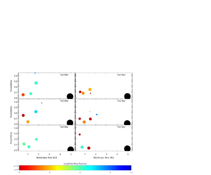
Figure 23: The left column shows the results of three simulations for different distribution of planetary embryos in a binary with equal-mass Sun-like stars. The orbit of the secondary star is circular with a radius of 30 AU. The right column shows the results of simulations for the same binary stars and similar distributions of planetary embryos where the secondary is in an orbit with a semimajor axis of 40 AU and eccentricity of 0.2 Hagh07 .

An interesting result shown in figure 22 is the relation between the orbital eccentricity of the stellar companion and the water content of the final bodies. As shown here, in systems where the secondary star has larger orbital eccentricity, the amount of water in final planets is smaller. This can be seen more clearly in figure 23, where the final assembly and water contents of planets are shown for a circular and an eccentric binary. As shown here, for identical initial distributions of planetary embryos (i.e., simulations on the same rows), the total water content of the system on the left, where the secondary star is in a circular orbit, is higher than that of the system on the right, where the orbit of the secondary is eccentric. This can be attributed to the fact that in an eccentric binary, because of the close approach of the secondary star to the disk of planetary embryos, most of the water-carrying objects at the outer regions of the disk leave the system prior to the formation of terrestrial planets Artymowicz94 ; David03 . Simulations indicate that on average 90% of embryos in these systems were ejected during the integration (i.e., their semimajor axes exceeded 100 AU) and among them, 60% collided with other protoplanetary bodies prior to their ejection from the system. A small fraction of embryos $(\sim 5\%)$ also collided with the primary or secondary star, or with the Jupiter-like planet of the system Hagh07 .

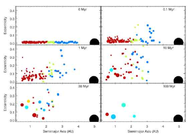
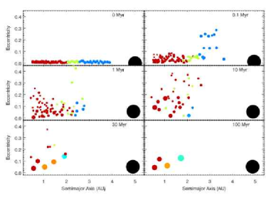
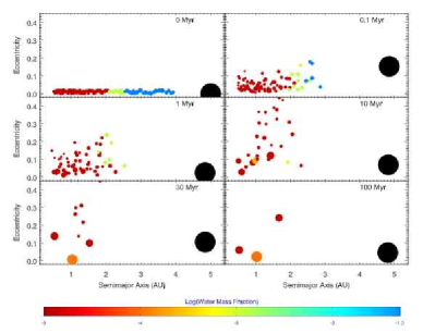
Figure 24: Variation of water contents of the final planets with the eccentricity of the stellar companion. In these simulations, the primary star has a mass of 0.5 solar-masses, the semimajor axis of the binary is 30 AU, and its eccentricity is equal to 0,0.2, and 0.4, from top to bottom Hagh07 .

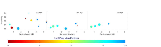
Figure 25: Habitable planet formation in binary systems with no Jupiter-like planet. The stars of each binary are Sun-like and their separations are 30 AU. The orbital eccentricity of the secondary star is 0, 0.2, and 0.4, for the systems on the left, middle, and right, respectively. Note that compared with previous simulations, the time of integration has to increase to 200 Myr in order to form comparable terrestrial-class planets Hagh07 .

In a binary-planetary system, the destabilizing effect of the secondary star is enhanced by the presence of the giant planet. Similar to our solar system, in these binaries, the Jovian-type planet perturbs the motion of embryos and enhances their radial mixing and the rate of their collisions by transferring angular momentum from the secondary star to these objects Chambers02-II ; Levison03 ; Raymond04 ; Raymond06a . Figure 24 shows this in more details. The binary systems in these simulations have mass-ratios of 0.5, and their secondary stars are at 30 AU. The binary eccentricity in these systems is equal to 0, 0.2 and 0.4, from top to bottom. As shown here, as the eccentricity of the binary increases, the interaction of the secondary star with the giant planet of the system becomes stronger (see the final eccentricity of the giant planet), which causes closer approaches of this object to the disk of planetary embryos and enhancing collisions and mixing among these bodies. The eccentricities of embryos, at distances close to the outer edge of the protoplanetary disk, rise to higher values until these bodies are ejected from the system. In binaries with smaller perihelia, the process of transferring angular momentum by means of the giant planet is stronger and the ejection of protoplanets occurs at earlier times. As a result, the total water budget of such systems is small. A comparison between figure 24 and figure 25, where simulations were carried out for a binary without a giant planet, illustrates the significance of the intermediate effect of the giant planet in a better way. As shown by figure 25, it is still possible to form terrestrial-class planets, with significant amount of water, in the habitable zone of the primary star. However, because of the lack of the transfer of angular momentum through the Jovian-type planet, the radial mixing of these objects is slower and terrestrial planet formation takes longer.

Another interesting result depicted by figure 25 is the decrease in the number of the final terrestrial planets and increase in their sizes and accumulative water contents with increasing the eccentricity of the secondary star. As shown here, from left panel to the right, as the binary eccentricity increases, the close approach of the secondary star to the protoplanetary disk increases the rate of the interaction of these objects and enhances their collisions and radial mixing. As a result, more of the water-carrying embryos participate in the formation of the final terrestrial planets. It is important to emphasize that this process is efficient only in moderately eccentric binaries. In binary systems with high eccentricities (small perihelia), embryos may be ejected from the system David03 , and terrestrial planet formation may become inefficient.

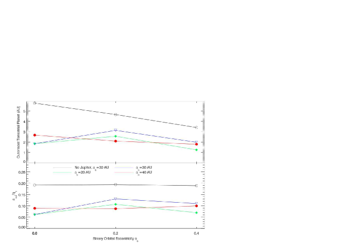
Figure 26: Top panel: Semimajor axis of the outermost terrestrial planet. Bottom panel: The ratio of the semimajor axis of this object to the perihelion distance of the binary. The secondary star is solar mass Hagh07 .

The results of the simulations without a giant planet imply a trend between the location of the outer terrestrial planet and the perihelion of the binary. In figure 26 this has been shown for a set of different simulations. The top panel in this figure represents the semimajor axis of the outermost terrestrial planet, $a_{\rm out}$, as a function of the binary eccentricity, $e_{b}$. The bottom panel shows the ratio of this quantity to the perihelion distance of the binary, $q_{b}$. As shown here, terrestrial planet formation in binaries without a giant planet seems to favor the region interior to approximately 0.19 times the binary perihelion distance. This has also been noted by Quintana07 (see their figure 9) in their simulations of terrestrial planet formation in close binary star systems. Given that the location of the inner edge of the habitable zone is at 0.9 AU, this trend implies that a binary perihelion distance of approximately 0.9/0.19 = 4.7 AU or larger may be necessary to allow habitable planet formation. According to these results, habitable planet formation may not succeed in binaries with Sun-like primaries that have stellar companions with perihelion distances smaller than $\sim$5 AU. This, of course, is not a stringent condition, and is neither surprising since a moderately close binary with a perihelion distance of $\sim$5 AU would be quite eccentric, and as indicated by Hol99 the orbit of a terrestrial-class object in the region around 1 AU from the primary of such a system will be unstable [see equation (1)].

In binary systems where a giant planet exist, figure 26 indicates that terrestrial planets form closer-in. The ratio $a_{\rm{out}}/q_{b}$ in these systems varies between approximately 0.06 and 0.13, depending on the orbital separation of the two stars. The accretion process in such systems is more complicated since the giant planet’s eccentricity and its ability to transfer angular momentum are largely regulated by the binary companion.

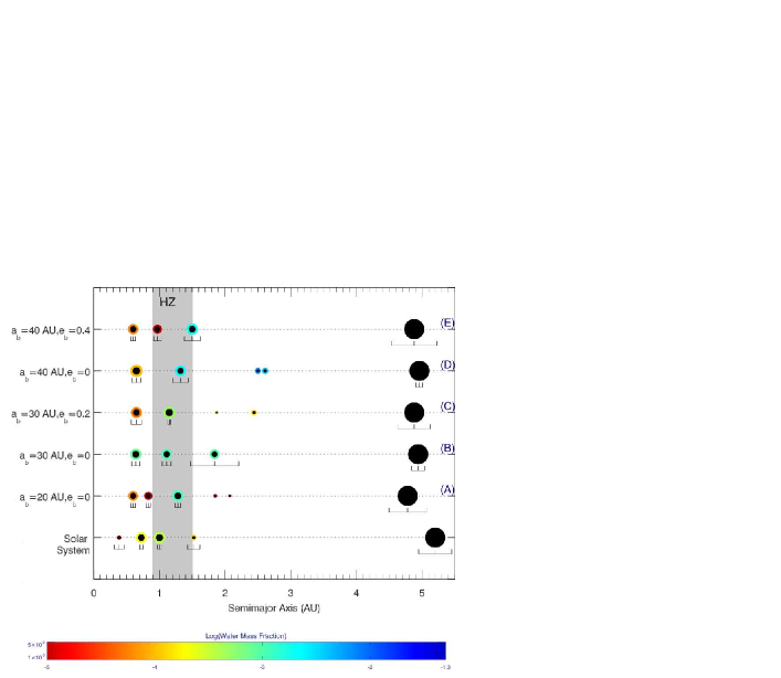
Figure 27: Variation of number and water content of Earth-like objects with the perihelion of the secondary star. The mass of the secondary star in all simulations is 1 solar-mass Hagh07 .

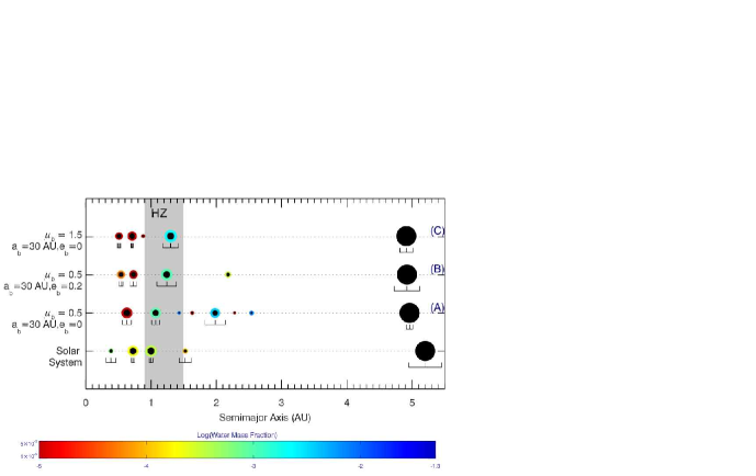
Figure 28: Variation of number and water content of Earth-like objects with the mass-ratio of the binary Hagh07 .

As shown by Hagh07 , despite the stochasticity of the simulations, and the large size of the parameter-space, many simulations resulted in the formation of Earth-like planet, with substantial amount of water, in the habitable zone of the primary star. Figures 27 and 28 show the result. The orbital elements of the final objects are given in Table 4. It is necessary to mention that because in these simulations, all collisions have been considered to be perfectly inelastic (i.e., the water contents of the resulted planets would be equal to the sum of the water contents of the impacting bodies, and the loss of water due to the impact and the motion of the ground of an impacted body Genda05 ; Canup06 has been ignored), the numbers given in Table 4 set an upper limit for the water budget of final planets. The total water budget of these objects may in fact be 5-10 times smaller than those reported here Raymond04 .

Table 4: (Sun’s habitable zone: 0.9 - 1.50 AU)

Simulation			${m_{p}}\,(M_{\oplus})$			$a_{p}$ (AU)			$e_{p}$			Water Fraction
9-A			0.95			1.28			0.03			0.00421
9-B			0.75			1.11			0.06			0.00415
9-C			1.17			1.16			0.03			0.00164
9-D			0.86			1.33			0.09			0.01070
9-E			0.95			1.50			0.08			0.00868
10-A			0.74			1.07			0.06			0.00349
10-B			0.99			1.26			0.12			0.00366
10-C			1.23			1.30			0.09			0.00103

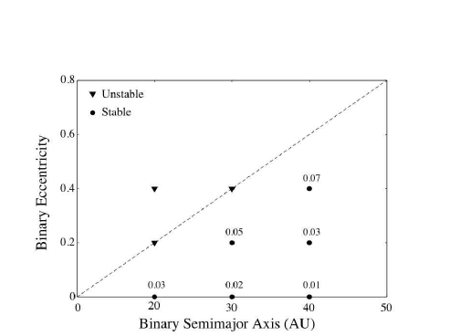
Figure 29: Habitable planet formation in the $({e_{b}},{a_{b}})$ space of an equal-mass binary-planetary system. Circles correspond to binaries in which habitable planets are formed. Triangles represent systems in which the giant planet is unstable. The number associated with each circle represents the average eccentricity of the giant planet of the system during the simulation Hagh07 .

A study of the systems of figures 27 and 28 indicates that these binaries have relatively large perihelia. Figure 29 shows this for simulations in a binary with a mass-ratio of 0.5 in terms of the semimajor axis and eccentricity of the stellar companion. The circles in this figure represent those systems in which the giant planet maintained a stable orbit and also simulations resulted in the formation of habitable bodies. The number associated with each circle corresponds to the average eccentricity of the giant planet during the simulation. The triangles correspond to systems in which the giant planet became unstable. Given that at the beginning of each simulation, the orbit of the giant planet was circular, a non-zero value for its average eccentricity is indicative of its interaction with the secondary star. The fact that Earth-like objects were formed in systems where the average eccentricity of the giant planet is small implies that this interaction has been weak. In other words, binaries with moderate to large perihelia and with giant planets on low eccentricity orbits are most favorable for habitable planet formation. Similar to the formation of habitable planets around single stars, where giant planets, in general, play destructive roles, a strong interaction between the secondary star and the giant planet in a binary-planetary system (i.e., a small binary perihelion) increases the orbital eccentricity of this object, and results in the removal of the terrestrial planet-forming materials from the system. For more details we refer the reader to Hagh07 .

References

- (1) Abe, Y., Ohtani, E., Okuchi, T., et al.: in Origin of the Earth and the Moon, Eds. Righter K. & Canup R., (Tucson: Univ. Arizona Press, 2000), 413
- (2) Abt, H. A.: AJ, 84, 1591 (1979)
- (3) Akeson, R. L., Koerner, D. W. & Jensen, E. L. N.: AJ, 505, 358 (1998)
- (4) Artymowicz, P. & Lubow, S. H.,: AJ, 421, 651 (1994)
- (5) Asghari, N., Broeg, C., Carone L. et al.: A&A, 426, 31 (2004)
- (6) Barbieri, M., Marzari, F. & Scholl, H.: A&A, 396, 219 (2002)
- (7) Benest, D.: A&A, 206, 143 (1988a)
- (8) Benest, D.: CMDA, 43, 47 (1988b)
- (9) Benest, D.: A&A, 223, 361 (1989)
- (10) Benest, D.: CMDA, 56, 45 (1993)
- (11) Benest, D.: A&A, 314, 983 (1996)
- (12) Benest, D.: A&A, 332, 1147 (1998)
- (13) Black, D.C.: AJ, 87, 1333 (1982)
- (14) Bodenheimer, P., Hubickyj, O. & Lissauer, J. J.: Icarus, 143, 2 (2000)
- (15) Bois, E., Kiseleva-Eggleton, L., Rambaux, N.& Pilat-Lohinger, E.: ApJ, 598,1312 (2003)
- (16) Broucke, R. A.: CMDA, 81, 321 (2001)
- (17) Campbell, B., Walker, G. A. H. & Yang, S.: AJ, 331, 902 (1988)
- (18) Canup, R. M., & Pierazzo, E.: 37th Annual Lunar and Planetary Science Conference, 2146 (2006)
- (19) Chambers, J. E., Quintana, E. V., Duncan, M. J. & Lissauer, J. J.: AJ, 123, 2884 (2002)
- (20) Chambers, J. E., & Cassen, P.: M&PS, 37, 1523 (2002)
- (21) Charnoz, S., Thébault, P., & Brahic, A.: A&A, 373, 683 (2001)
- (22) Capen, S., Haghighipour, N. & Kirste, S.: to appear in BAAS (2009)
- (23) David, E., Quintana, E. V., Fatuzzo, M., & Adams, F. C.: PASP, 115, 825 (2003)
- (24) Deprit, A. & Rom, A.: A&A, 5 416 (1970)
- (25) Diakov, B. B. & Reznikov, B. I. : Moon. Planet., 23, 429 (1980)
- (26) Domingos, R. C., Winter, O. C. & Yokoyama, T.: MNRAS, 373, 1227 (2006)
- (27) Donnison, J.R. & Mikulskis, D.F.: MNRAS, 266, 25 (1994)
- (28) Drobyshevski, E. M.: Moon. Planet., 18, 145 (1978)
- (29) Duquennoy, A.& Mayor, M.: A&A, 248, 485 (1991)
- (30) Dvorak, R.: Celest. Mech., 34, 369 (1984)
- (31) Dvorak, R.: A&A, 167, 379 (1986)
- (32) Dvorak, R., Froeschlé, Ch., & Froeschlé, C.: A&A, 226, 335 (1989)
- (33) Dvorak, R.& Lohinger, E.: Proceedings of the NATO ASI Series, Roy A.E. (Ed.), Plenum Press, New York and London, 439 (1991)
- (34) Dvorak, R. & Freistetter, F.: in Dvorak, Freistetter, Kurths (eds.) Chaos and Stability in Planetary Systems, Springer LNP 683 50 (2003)
- (35) Dvorak, R., Pilat-Lohinger, E., Funk, & B., Freistetter, F.:A&A, 398, L1 (2003)
- (36) Dvorak, R., Pilat-Lohinger E., Funk B.& Freistetter F.: A&A, 410, L13-L16 (2003)
- (37) Dvorak, R., Pilat-Lohinger, E., Bois, E. et al.: RevMexAA (Series de Conferencias), 21, 222 (2004)
- (38) Dvorak, R., Pilat-Lohinger, E., Schwarz, R., & Freistetter, F.: A&A, 426, 37 (2004)
- (39) Eggenberger, A., Udry, S., & Mayor, M.: in Scientific Frontiers in Research on Extrasolar Planets, ASP Conference Series, Eds. Deming, D. & Seager, S. (San Francisco, 2001), 294, 43
- (40) Érdi, B. & A. Pál, A.: Dynamics of resonant exoplanetary systems,in: Proceedings of the 3rd Austrian-Hungarian Workshop on Trojans and related Topic, Eds. F. Freistetter, R. Dvorak. & B.Érdi (Eötvös University Press), pp.3 (2003)
- (41) Érdi, E., Dvorak, R., Sándor, Zs.& Pilat-Lohinger, E.: MNRAS 351,1943 (2004)
- (42) Érdi, B., & Sándor, Zs.: CMDA, 92, 113 (2005)
- (43) Érdi, B., Fröhlich, G., Nagy, I., & Sándor, Zs.: in Proceedings of the 4th Austrian Hungarian Workshop on celestial mechanics, Eds. Á. Süli, F. Freistetter, & A. Pál, 85 (2007)
- (44) Fatuzzo, M., Adams, F. C., Gauvin, R. & Proszkow, E. M.: PASP, 118, 1510 (2006)
- (45) Forget, F. & Pierrehumbert, R. T.: Science, 278, 1273 (1997)
- (46) Froeschlé, C., Lega, E. & Gonczi, R.: CMDA, 67, 41 (1997)
- (47) Fuhrmann, K.: Astron. Nachr., 325, 3 (2004)
- (48) Funk, B., Pilat-Lohinger, E., Dvorak, R., Freistetter, F.& Erdi, B.: CMDA, 90, 43 (2004)
- (49) Genda, H., & Abe, Y.: 36th Annual Lunar and Planetary Science Conference, 2265 (2005)
- (50) Gayon, J., & Bois, E.: A&A, 482, 665
- (51) Graziani, F. & Black, D.C.: ApJ, 251, 337 (1981)
- (52) Griffin, R. F., Carquillat, J. M. & Ginestet, N.: The Observatory, 122, 90 (2002)
- (53) Haghighipour, N.: in AIP Conference Proceedings 713: The Search for Other Worlds, Eds. S. S. Holt, & D. Deming (New York, 2004) pp.269
- (54) Haghighipour, N.: BAAS, 37 526 (2005)
- (55) Haghighipour, N.: astro-ph/0509659
- (56) Haghighipour, N.: ApJ, 644, 543 (2006)
- (57) Haghighipour, N. & Raymond, S. N.: ApJ, 666, 436 (2007)
- (58) Haghighipour, N., Steffen, J., Hinse, T., & Agol, A.: Am. Geophys. U., P14B-04 (2008)
- (59) Hagle, J. & Dvorak, R.: Celest. Mech., 42, 355 (1988)
- (60) Harrington, R.S.: Celest. Mech., 6, 322 (1972)
- (61) Harrington, R.S.: AJ, 80, 1081 (1975)
- (62) Harrington, R.S.: AJ, 82, 753 (1977)
- (63) Hatzes, A. P., Cochran, W. D., Endl, et al.: ApJ, 599, 1383 (2003)
- (64) Hayashi, C.: Prog. Theor. Phys. Suppl., 70, 35 (1981)
- (65) Hénon, M. & Guyot, M.: in Periodic Orbits, Stability and Resonances, Eds. Giacaglia G. E. O., & D. Reidel, D., Pub. Comp. (Netherlands, 1970) pp.349
- (66) Heppenheimer, T. A.: Icarus, 22, 436 (1974)
- (67) Heppenheimer, T. A.: A&A, 65, 421 (1978)
- (68) Holman, M. J., Touma, J.& Tremaine, S.: Nature, 386, 254 (1997)
- (69) Holman M. J. & Wiegert P. A.: AJ, 117, 621 (1999)
- (70) Innanen, K. A., Zheng, J. Q., Mikkola, S.& Valtonen, M. J.: AJ, 113, 1915 (1997)
- (71) Jewitt D., & Haghighipour, N.: ARA&A, 45, 261 (2007)
- (72) Jones, B. W., Sleep, P. N., Chamber, J. R.: A&A, 366, 254 (2001)
- (73) Jones, B. W., Underwood, D. R. & Sleep, P. N.: ApJ, 622, 1091 (2005)
- (74) Jones, B. W., Sleep, P. N. & Underwood, D. R.: 2006, ApJ, 649, 1010 (2006)
- (75) Kasting, J. F., Whitmire, D. P. & Reynolds, R. T.: Icarus, 101, 108 (1993)
- (76) Kokubo, E., & Ida, S.: Icarus, 131, 171 (1998)
- (77) Kortenkamp, S. J., Wetherill, G. W. & Inaba, S.: Science, 293, 1127 (2001)
- (78) Kozai, Y.: AJ, 67, 591 (1962)
- (79) Krist, J. E., Stapelfeldt, K. R., Golimowski, D. A., et al.: AJ, 130, 2778 (2005)
- (80) Kubala, A., Black, D. C. & Szebehely, V.: CMDA, 56, 51 (1993)
- (81) Laughlin, G., & Chambers, J. E.: AJ, 124, 592 (2002)
- (82) Levison, H. F., & Agnor, C.: AJ, 125, 2692 (2003)
- (83) Lissauer, J. J., Quintana, E. V., Chambers, J. E., et al.: RevMexAA (Series de Conferencias), 22, 99 (2004)
- (84) Lodders, K., & Fegley, B., Jr.: M & PS, 33, 871 (1998)
- (85) Lohinger, E.& Dvorak, R.: A&A, 280, 683 (1993)
- (86) Malmberg, D., Davies, M. B. & Chambers, J. E.: MNRAS, 377, L1 (2007)
- (87) Marchal, C.: The Three-Body Problem (Elsevier, 1990), pp.49
- (88) Marzari, F., Scholl, H., Tomasella, L. & Vanzani, V.: Planet. & Sp. Sci., 45, 337 (1997)
- (89) Marzari, F. & Scholl, H.: ApJ, 543, 328 (2000)
- (90) Marzari, F., Thébault, P., & Scholl, H.: Submitted to A&A (arXiv: 0908.0803v2)
- (91) Mathieu, R. D.: ARA& A, 32, 465 (1994)
- (92) Mathieu, R. D., Ghez, A. M., Jensen, E. L. & Simon, M.: in Protostars and Planets IV, Eds. Mannings V., Boss A. P. & Russell S. S., (Univ. Arizona Press, Tucson 2000), pp 703
- (93) Mayor, M., & Queloz, D.: Nature, 378, 355 (1995)
- (94) Menou, K., & Tabachnik, S.: ApJ, 583, 473 (2003)
- (95) Mischna, M. A., Kasting, J. F., Pavlov, A. & Freedman, R.: Icarus, 145, 546 (2000)
- (96) Morbidelli, A., Chambers, J., Lunine, J. I., et al.: MAPS, 35, 1309 (2000)
- (97) Moriwaki, K. & Nakagawa, Y.: ApJ, 609, 1065 (2004)
- (98) Musielak, Z. E., Cuntz, M., Marshall, E. A., & Stuit, T. D.: A&A, 434, 355 (2005)
- (99) Nauenberg, M.: AJ, 124, 2332 (2002)
- (100) Neuhäuser, R., Mugrauer, M., Fukagawa, M., et al.: A&A, 462, 777 (2007)
- (101) Norwood, J. W. & Haghighipour, N.: BAAS, 34, 892 (2002)
- (102) Paardekooper, S. J., Thébault, P., & Mellema, G.: MNRAS, 386, 973 (2008)
- (103) Pál, A. & Sándor, Zs.: in Proceedings of the 3rd Austrian-Hungarion Workshop on Trojans and related topics, Eds. F. Freistetter, R. Dvorak, & B. Érdi, pp.25 (2003)
- (104) Pendleton, Y. J. & Black, D. C.: AJ, 88, 1415 (1983)
- (105) Pichardo, B., Sparke, L. S. & Aguilar, L. A. : MNRAS, 359, 521 (2005)
- (106) Pilat-Lohinger, E., Suli, A., Freistetter, F., et al.: 2006, in Epsc. conf., European Planetary Science Congress (Berlin 2006), pp. 717
- (107) Pilat-Lohinger, E. & Dvorak, R.: CMDA, 82, 143 (2002)
- (108) Pilat-Lohinger, E., Funk, B., Dvorak, R.: A&A, 400, 1085 (2003)
- (109) Pilat-Lohinger, E., Dvorak, R., Bois, E. & Funk, B.: in APS Conference Series 321: Extrasolar Planets: Today and Tomorrow, Eds. Beaulieu J. P., Lecavelier des Etangs A. & Terquem C., pp.410 (2004)
- (110) Pilat-Lohinger, E.: 2005, in “Dynamics of Populations of Planetary Systems”, Proceedings of IAU Coll. 197, eds. Knezevic Z.& Milani A. (Cambridge University Press, 2005), pp.71
- (111) Pilat-Lohinger E.& Funk, B.: in Proceedings of the 4th Austro-Hungarian Workshop (Budapest, 2006)
- (112) Quintana, E. V., Lissauer, J. J., Chambers, J. E. & Duncan, M. J.: ApJ, 576, 982 (2002)
- (113) Quintana, E. V. & Lissauer, J. J.: Icarus, 185, 1 (2006)
- (114) Quintana, E. V., Adams, F. C., Lissauer, J. J. & Chambers, J. E.: ApJ, 660, 807 (2007)
- (115) Rabe, E.: AJ, 66, 500 (1961)
- (116) Rabl, G.& Dvorak, R.: A&A, 191, 385 (1988)
- (117) Raghavan, D., Henry, T. J., Mason, B. D., et al.: ApJ, 646, 523 (2006)
- (118) Raymond, S. N., Quinn, T., & Lunine, J., I.: Icarus, 168, 1 (2004)
- (119) Raymond, S. N., Quinn, T., & Lunine, J., I.: ApJ, 632, 670 (2005)
- (120) Raymond, S. N., Quinn, T., & Lunine, J., I.: Icarus, 177, 256 (2005)
- (121) Raymond, S. N.: ApJL, 643, L131 (2006)
- (122) Raymond, S. N., Barnes, R., & Kaib, N. A.: ApJ, 644, 1223 (2006)
- (123) Raymond, S. N., Mandell, A. M., & Sigurdsson, S.: Science, 313, 1413 (2006)
- (124) Raymond, S. N., Quinn, T., & Lunine, J.I.: Astrobiology, 7, 66 (2007)
- (125) Rodriguez, L. F., D’Alessio, P., Wilner, D. J., et al.: Nature, 395, 355 (1998)
- (126) Saleh, L. A., & Rasio, F. A.: ApJ, 694, 1566 (2009)
- (127) Sándor, Zs. & Érdi, B.: CMDA, 86, 301 (2003)
- (128) Sandor, Zs., Suli., A., Erdi, B. et al.: MNRAS, 374, 1495 (2006)
- (129) Schwarz, R. , Pilat-Lohinger, E., Dvorak, R. et al.: Astro. Bio., 5, 579 (2005)
- (130) Schwarz, R.: Ph.D. thesis, University of Vienna, online database: http://media.obvsg.at/dissdb (2005)
- (131) Schwarz, R., Dvorak, R., Pilat Lohinger, E., et al.: A&A, 462, 1165 (2007)
- (132) Schwarz, R., Dvorak, R., Süli, Á., & Érdi, B.: A&A, 474 1023 (2007)
- (133) Schwarz, R., Süli, Á., & Dvorak, R.: MNRAS, 398 2085 (2009)
- (134) Silbert, J., Gledhill, T., Duchéne, G. & Ménard, F.: ApJ, 536, L89 (2000)
- (135) Szebehely, V.: Celest. Mech., 22, 7 (1980)
- (136) Szebehely, V. & McKenzie, R.: Celest. Mech., 23, 3 (1981)
- (137) Szebehely, V.: Celest. Mech., 34, 49
- (138) Takeda, G. & Rasio, F. A.: Astrophy. & Sp. Sci., 304, 239 (2006)
- (139) Takeda, G., Kita, R., & Rasio, F. A.: ApJ, 683, 1063 (2008)
- (140) Thébault, P., Marzari, F., Scholl, et al.: A&A, 427, 1097 (2004)
- (141) Thébault, P., Marzari, F. & Scholl, H.: Icarus, 183, 193 (2006)
- (142) Thébault, P., Marzari, F. & Scholl, H.: MNRAS, 388, 1528 (2008)
- (143) Thébault, P., Marzari, F. & Scholl, H.: MNRAS, 393, L21 (2009)
- (144) Torres, G: ApJ, 654, 1095 (2007)
- (145) Trilling, D. E., Stansberry, J. A., Stapelfeldt, K. R., et al.: ApJ, 658, 1264 (2007)
- (146) Verrier, P. E. & Evans, N. W.: MNRAS, 368, 1599 (2006)
- (147) White, R. J., Ghez, A. M., Reid, I. N. & Schultz, G.: ApJ, 520, 811 (1999)
- (148) White, R. J. & Ghez, A. M.: ApJ, 556, 265 (2001)
- (149) Whitmire, D. P., Matese, J. L., Criswell, L. & Mikkola, S.: Icarus, 132, 196 (1998)
- (150) Wiegert, P. A. & Holman, M. J.: ApJ, 113, 1445 (1997)
- (151) Wetherill, G. W.: Icarus, 119, 219 (1996)
- (152) Williams, D. M. & Kasting, J. F.: Icarus, 129, 254 (1997)
- (153) Xie, J. W., & Zhou, J. L.: ApJ, 686, 570 (2008)
- (154) Xie, J. W., & Zhou, J. L.: ApJ, 698, 2066 (2009)
- (155) Ziglin, S. L.: Sov. Astron. Let., 1, 194 (1975)
- (156) Zucker, S., Mazeh, T., Santos, N. C., et al.: A&A 426, 695 (2004)
Index