Self-trapping of a Fermi super-fluid in a double-well potential in the BEC-unitarity crossover

Abstract

We derive a generalized Gross-Pitaevskii density-functional equation appropriate to study the Bose-Einstein condensate (BEC) of dimers formed of singlet spin-half Fermi pairs in the BEC-unitarity crossover while the dimer-dimer scattering length $a$ changes from 0 to $\infty$. Using an effective one-dimensional form of this equation, we study the phenomenon of dynamical self-trapping of a cigar-shaped Fermi super-fluid in the entire BEC-unitarity crossover in a double-well potential. A simple two-mode model is constructed to provide analytical insights. We also discuss the consequence of our study on the self-trapping of an atomic BEC in a double-well potential.

I Introduction

After the experimental realization of Bose-Einstein condensate (BEC) and its controlled study under different trapping conditions book , there have been many interesting experiments with a cigar-shaped BEC in a quasi one-dimensional (1D) trap with a tight transverse confinement gor . Along the axial direction several different types of traps have been employed: harmonic book , double-well GatiJPB2007 , periodic optical-lattice kast , and bichromatic optical-lattice bich traps. Many novel phenomena have been predicted and observed in such quasi-1D setting. Of these, the ones worth mentioning include the formation of bright bright , gap gap , and dark dark solitons, self-trapping trappingPRL ; GatiJPB2007 and Josephson oscillation GatiJPB2007 ; cataliotti ; joseBEC .

Macroscopic dynamical self-trapping and Josephson oscillation were predicted theoretically java ; trappingPRL ; Gong ; OstrovskayaPRA2000 ; TS and observed experimentally cataliotti ; GatiJPB2007 . Josephson effect was observed in super-fluid (SF) ³He He3 and ⁴He He4 . After the experimental observation of BEC in a optical-lattice trap cataliotti , controlled studies of Josephson oscillation and self-trapping in a cigar-shaped BEC seems well under control GatiJPB2007 . The studies of such phenomena in a cigar-shaped BEC usually employ a double-well potential GatiJPB2007 . In the simplest case of such a symmetric 1D potential with the origin of the axial coordinate $x$ set at the trap center, under certain initial conditions, when a BEC is released with a population imbalance between two sides of $x=0$, it executes undamped Josephson oscillation on both sides of the trap center maintaining a time-averaged population imbalance equal to zero. Under different initial conditions, the BEC exhibits self-trapping, occupying preferably one side of the trap, thus maintaining a definite non-zero value of time-averaged population imbalance. The understanding of the transition from Josephson oscillation to self-trapping and vice versa has been the topic of many recent investigations GatiJPB2007 .

A SF Fermi gas in a double-well potential is perhaps even more interesting, nevertheless much less studied sala . (There have been studies of Josephson oscillation of a Fermi gas in a OL potential ferop ). Such a trapped SF Fermi gas gives us the unique opportunity to study the Bardeen-Cooper-Schrieffer (BCS) to BEC crossover in a two-component Fermi gas under an entirely different set-up. The BCS-BEC crossover can be realized by varying the attraction between the spin-half fermions forming pairs using the Feshbach resonance technique. As the attraction is increased from zero, the simple BCS SF turns into a complex Cooper-pair-induced strongly interacting SF and at unitarity (when the Fermi-Fermi scattering length $a_{f}$ tends to infinity), it is possible for the Cooper pairs to turn spontaneously into Fermi dimers (two-body bound state of fermionic atoms) and the BCS SF turns into a BEC of dimers.

After the experimental realization exp23 of the BCS-BEC crossover in a trapped Fermi SF by varying the atomic interaction near a Feshbach resonance, there have been renewed interests exp10 ; DF2 ; rmp2 in the study of a Fermi SF at unitarity and beyond in the BEC region where we have the BEC of dimers. One can thus recover the bosonic behavior in the BEC limit of the crossover (when the dimer-dimer scattering length $a$ tends to zero), while expecting new and distinct behavior in the vicinity of the unitarity regime. Moreover, on the experimental front it is easier to realize a controlled BEC-unitarity crossover (BEC side of the BCS-BEC crossover) of the Fermi SF than the BCS-unitarity crossover (BCS side of the BCS-BEC crossover), as the super-fluid transition temperature in the BCS side of the crossover is very low and difficult to achieve.

Here we present a unified Galilean-invariant dynamical equation for the study of the BEC-unitarity crossover of a cigar-shaped BEC of dimers formed of Fermi atoms. In the BEC limit of small dimer-dimer scattering length $a,$ the present equation reduces to the usual Gross-Pitaevskii (GP) equation GP for bosons, and in the unitarity limit it yields a density-functional (DF) equation DFT for fermions. Hence we call this equation a DF GP equation for a Fermi SF valid in the BEC-unitarity crossover. For the study of a cigar-shaped Fermi SF along the BEC-unitarity crossover, we reduce the present DF GP equation to a quasi-1D form and use this reduced equation to the study of the self-trapping of Fermi SF in a double-well potential. This analytic development is presented in Sec. II. This reduced equation also describes an atomic BEC with repulsive atomic interaction in the BEC-unitarity crossover with different numerical value(s) of certain parameter(s), and hence the results of the present investigation are also applicable to the self-trapping of a repulsive BEC in a double-well potential.

The numerical simulation with the time-dependent quasi-1D equation for a cigar-shaped Fermi SF in a symmetric double-well potential with an initial population imbalance between two wells reveals interesting features of the Josephson oscillation and self-trapping across the BEC-unitarity crossover. In the limit of zero nonlinearity one has AC Josephson oscillation. As nonlinearity is increased by increasing the dimer-dimer scattering length or the number of particle, the Josephson oscillation stops and self-trapping emerges for a double-well potential with appropriate parameters. With further increase of nonlinearity self-trapping is destroyed and the population in the two wells executes irregular oscillation. For very large nonlinearity, however, the regular Josephson oscillation comes back. Nevertheless, for a small number of particles, the critical nonlinearity required for one of these phenomenon may not be attained and that particular phenomenon may not be realized. (The nonlinearity actually saturates for a large value of $a$ and hence cannot be arbitrarily increased by increasing $a$ as one approaches unitarity for a small number of atoms.) These features are discussed in detail in Sec. IV where we present the numerical results.

In Sec. III we present a simple analytic two-mode model to understand the essential features of the numerical results reported in Sec. IV and also point out the limitation of the two-mode model. Finally, in Sec. V we present a brief summary and conclusion of the present investigation.

II DF GP equation for a Fermi SF in the BEC-unitarity crossover

At unitarity the following density-functional (DF) equation for trapped SF fermions AS2 ; AS3 has produced results for energy in close agreement with independent Monte-Carlo calculations MC

$$\left[-\frac{\hbar^{2}}{2m}\nabla^{2}+U+\mu(n)-i\frac{\partial}{\partial t}\right]\Psi({\bf r},t)=0,$$ (1)

where $U$ is the trapping potential, $m$ is the mass of a dimer (twice the atomic mass), $\mu(n)=\xi\hbar^{2}n^{2/3}/m$ is the bulk chemical potential of dimers with density (of dimers) $n=|\Psi|^{2}$, and $\xi=2(6\pi^{2})^{2/3}\zeta$. The normalization condition of the DF wave function is $\int|\Psi|^{2}d^{3}r=N$, where $N$ is the number of dimers. At unitarity the only length scale is $n^{-1/3}$, and from dimensional argument the chemical potential $-$ and all energies of the trapped SF fermions $-$ have the above universal form uni .

There have been many theoretical the1 ; the2 and experimental exp investigations which extracted the value of the constant $\zeta$ for fermions, and the most accurate value of this constant is given by independent Monte-Carlo calculations by two groups the1 : $\zeta\approx 0.44$, consequently, $\xi\approx 13.37$ and we shall use this value of $\xi$ in the present study. For a trapped atomic BEC, the energy and chemical potential have the same universal form: $\sim\xi\hbar^{2}n^{2/3}/m$ cow , where now mass $m$ and density $n$ refer to bosons. For fundamental bosonic atoms, microscopic numerical calculation based on Jastrow variational wave function yielded for the constant $\xi$ a slightly different value $\xi=22.22$ cow . With this modification in the value of $\xi$, the present investigation could be applied to the study of self-trapping of an atomic BEC.

At unitarity the Fermi pair can stay as a Cooper pair or a dimer and transform into each other without transfer of energy and Eq. (1) can describe both the Cooper pair and dimer phases. Here we interpret Eq. (1) as the equation for dimers. At unitarity the scattering length $a$ of two dimers goes to infinity: $a\to\infty$. (Actually, at unitarity, the scattering length of two Fermi atoms $a_{f}\to\infty$. Model studies have indicated that $a\propto a_{f}$ petrov . Consequently, at unitarity we take $a\to\infty$.)

Although Eq. (1) describes both the dimer SF and the Cooper-pair induced BCS SF at unitarity, the bulk chemical potential $\mu(n)$ appearing in this equation should be interpreted differently. For the BCS SF it originates from the kinetic energy of Fermi atoms put in different quantum orbitals consistent with the Pauli principle discounted for by the negative attractive energy due to atomic interaction. For the dimer SF it originates solely from the repulsive interaction energy among dimers. In the BCS limit as $a_{f}\to 0^{-}$ we have the finite nonlinear term $\mu(n)=2E_{F}=2(6\pi^{2})^{2/3}\hbar^{2}n^{2/3}/m$ AS2 in Eq. (1) originating from the kinetic energy of Fermi atoms with negligible contribution from inter-atomic attraction. On the other hand, in the BEC limit as $a\to 0^{+}$ the nonlinear term for dimers reduces to zero and at unitarity the nonlinear term in Eq. (1) originates from the saturation of repulsive dimer-dimer interaction as $a\to\infty$.

For the Fermi SF of dimers (and also for an atomic BEC) in the BEC-unitarity crossover the following two leading terms of the bulk chemical potential of a dilute uniform gas can be obtained nilsen from the expression for energy per particle as obtained by Lee, Huang, and Yang lee

$$\mu(n,a)=({4\pi\hbar^{2}an}/{m})\left(1+\alpha(n^{1/3}a)^{3/2}+...\right),$$ (2)

where $\alpha=32/(3\sqrt{\pi})$ and $n^{1/3}a$ is the dimensionless gas parameter. In this expression the scattering length $a$ must be positive ($a>0$) corresponding to a repulsive interaction. Higher-order terms of expansion (2) has also been considered bra ; the lowest order term was derived by Lenz lenz . Considering only the lowest-order term in expansion (2), appropriate in the BEC limit as $a,a_{f}\to 0^{+}$, the dimers obey the usual GP equation GP

$$\biggr{[}-\frac{\hbar^{2}}{2m}\nabla^{2}+U+\frac{4\pi\hbar^{2}a}{m}|\Psi|^{2}-i\frac{\partial}{\partial t}\biggr{]}\Psi({\bf r},t)=0\,.$$ (3)

Considering the second term in the expansion (2), in the BEC limit, the following modified GP equation for dimers can be written following the suggestion of Fabrocini and Polls polls

$$\biggr{[}-\frac{\hbar^{2}}{2m}\nabla^{2}+U+\frac{4\pi\hbar^{2}a}{m}|\Psi|^{2}\left(1+\alpha a^{3/2}|\Psi|\right)$$

$$-i\frac{\partial}{\partial t}\biggr{]}\Psi({\bf r},t)=0\,.$$ (4)

Equation (II) provides an adequate correction to the GP equation (3) for small $a$. But as $a$ increases and diverges at unitarity, the nonlinear term should saturate to the finite universal nonlinear term $\mu(n)$ of Eq. (1) and not diverge like the nonlinear terms of the GP equation (3) and of the Fabrocini-Polls equation (II). The chemical potential and energy should not diverge at unitarity, as the interaction potential remains finite in this limit, although the scattering length $a$ diverges. In the weak-coupling GP limit, the scattering length serves as a faithful measure of interaction. But as $a$ increases, it ceases to be a measure of interaction. For a general scattering length, an exact expression of the chemical potential is not available. However, a recent quantum Monte Carlo study maps out the equation of state in the entire BEC-BCS crossover regime the1 .

Following a recent suggestion AS1 , for the full BEC-unitarity crossover we consider the DF GP equation for the dimer SF providing a smooth interpolation between Eqs. (1) and (II):

$$\biggr{[}-\frac{\hbar^{2}\nabla^{2}}{2m}+U+\mu(n,a)-i\frac{\partial}{\partial t}\biggr{]}\Psi({\bf r},t)=0\,,$$ (5)

$$\mu(n,a) = \frac{4\pi\hbar^{2}a}{m}|\Psi|^{2}$$ (6)

$$\times \left(\frac{1+\alpha(1+\delta)a^{3/2}|\Psi|}{1+\alpha\delta a^{3/2}|\Psi|+\gamma(1+\delta)a^{5/2}|\Psi|^{5/3}}\right)\,,$$

where $n=|\Psi|^{2}$ and $\delta$ and $\gamma$ are yet unknown constants satisfying $\gamma=4\pi\alpha/\xi$. (These equations are also valid for an atomic BEC with $m$ and $a$ representing atomic mass and scattering length, respectively, and with $\xi=22.22$ cow .) By construction, Eq. (6) yields the limit (2) for small $a$; it also has the correct behavior at unitarity. Using a similar expression for $\mu(n,a)$ in the BCS-unitarity crossover ska the constant $\delta$ was calculated sadhan by requiring that the first derivative of $\mu(n,a)$ with respect to $(an^{1/3}$) be continuous at unitarity. The condition for continuity yields a small value for $\delta(\sim 0.04)$. However, we shall take $\delta=0$ in this study. This will make further analytical development easier while maintaining the first derivative of $\mu(n,a)$ with respect to $(an^{1/3}$) approximately continuous at unitarity. A set of equations, similar to Eqs. (5) and (6), for fundamental bosons, and not for composite dimers, produced results for energy AS2 of a trapped condensate in agreement with Monte-Carlo calculations MCBOSE . A similar equation for the BCS-unitarity crossover produced results for energy AS2 ; ska of a trapped BCS SF in agreement with Monte-Carlo calculations MCBCS . Different parametrization of the chemical potential in the BEC-BCS crossover have been proposed in the literature chempot . We do not expect our results in this work will be sensitive to which specific form for $\mu(n,a)$ we choose to use here. Furthermore, it has been shown that the DF GP equation (5) is equivalent to the quantum hydrodynamic equations for dimers AS2 ; chempot

$$\frac{\partial n}{\partial t}+\nabla\cdot(n{\bf v})=0\,,$$

$$m\frac{\partial{\bf v}}{\partial t}+\nabla\biggr{[}-\frac{\hbar^{2}}{2m}\frac{\nabla^{2}\sqrt{n}}{\sqrt{n}}+\frac{mv^{2}}{2}+U+\mu(n,a)\biggr{]}=0\,,$$

if we identify

$$\Psi({\bf r},t) = \sqrt{n({\bf r},t)}\,e^{is({\bf r},t)}\,,$$

$${\bf v} = \hbar\nabla s/m\,,$$

where $s$ is a phase, and $\bf v$ is the velocity.

For a cigar-shaped SF, where the transverse trapping is very strong, the interesting dynamics is confined in the axial direction and in the transverse direction the system is confined in its ground state. In such a quasi-1D geometry, the axial and transverse coordinates decouple and it is useful to write an effective 1D equation for the dynamics of a cigar-shaped SF and we perform the same in the following. For the cigar-shaped double-well trap,

$$U({\bf r}) = V(x)+m\omega^{2}(x^{2}+\lambda^{2}z^{2}+\lambda^{2}y^{2})/2\,,$$

$$V(x) = A\hbar\omega\exp(-\kappa m\omega x^{2}/\hbar)\,,$$

where $\lambda\gg 1$, and $A$ and $\kappa$ are two dimensionless parameters characterizing the strength and width of the barrier, respectively, it is appropriate to take $\Psi({\bf r},t)=\psi(x,t)\phi(y)\phi(z)$ with $\phi(y)=[m\omega\lambda/(\hbar\pi)]^{1/4}\exp[-m\omega\lambda y^{2}/(2\hbar)]$ representing the harmonic-oscillator ground state in the transverse direction and $\psi(x,t)$ representing the essential dynamics in the $x$ direction. The potential $V(x)$ together with the harmonic trap $m\omega^{2}x^{2}/2$ simulate a double-well in the axial $x$ direction. Multiplying Eqs. (1) and (II) by $\phi(y)\phi(z)$ and integrating over $y$ and $z$ we get the following 1D equations AS3 ; cigar

$$\biggr{[}-\frac{1}{2}\frac{\partial^{2}}{\partial x^{2}}+U(x)+\xi\frac{3}{5}\left(\frac{\lambda n}{\pi}\right)^{2/3}-i\frac{\partial}{\partial t}\biggr{]}\psi(x,t)=0,$$ (7)

$$\biggr{[}-\frac{1}{2}\frac{\partial^{2}}{\partial x^{2}}+U(x)+2a\lambda n\left(1+\alpha a^{3/2}\frac{4}{5}\frac{\sqrt{n\lambda}}{\sqrt{\pi}}\right)$$

$$-i\frac{\partial}{\partial t}\biggr{]}\psi(x,t)=0,$$ (8)

where ${{n=|\psi(x,t)|^{2}}},U(x)=Ae^{-\kappa x^{2}}+{x^{2}}/{2}$ represents the double-well potential and $n=|\psi|^{2}$ and we use harmonic oscillator dimensionless units $\hbar=m=\omega=1$. All lengths are now expressed in oscillator unit $\sqrt{\hbar/(m\omega)}$ and time in $\omega^{-1}$, and $\psi$ is normalized as $\int_{-\infty}^{\infty}dx|\psi(x,t)|^{2}=N$.

A simple DF GP equation interpolating between Eqs. (7) and (II) is

$$\biggr{[}-\frac{1}{2}\frac{\partial^{2}}{\partial x^{2}}+U(x)+\mu(n,a)-i\frac{\partial}{\partial t}\biggr{]}\psi(x,t)=0\,,$$ (9)

$$\mu(n,a)=2a\lambda n\left(\frac{1+\frac{4}{5}\frac{\sqrt{\lambda}}{\sqrt{\pi}}\alpha a^{3/2}\sqrt{n}}{1+\beta a^{5/2}n^{5/6}}\right)\,,$$ (10)

where $n=|\psi|^{2}$ and $\beta=8\alpha\lambda^{5/6}\pi^{1/6}/(3\xi)$. Equation (9) reduces in the BEC $a\to 0^{+}$ limit to Eq. (II) and in the unitarity $a\to\infty$ limit to Eq. (7). We shall use Eq. (9) for the description of self-trapping and Josephson oscillation in the BEC-unitarity crossover of fermions.

III Two-Mode Model of the Fermi SF

III.1 Two-Mode Model

Before we present the full numerical results, it is instructive to consider the so-called two-mode model trappingPRL which is widely used in the study of BEC in a double-well potential, and more recently, has been used in the investigation of Fermi SF across a weak link newref . Due to its simplicity, the two-mode model can provide many useful insights. Here we construct the corresponding two-mode model of the Fermi SF based on Eq. (9).

To this end, we decompose $\psi(x,t)$ as

$$\psi(x,t)=\psi_{1}(t)\phi_{1}(x)+\psi_{2}(t)\phi_{2}(x)\,,$$ (11)

where the spatial mode functions $\phi_{1,2}(x)$ are assumed to be real, satisfy the orthonormal condition

$$\int\phi_{i}(x)\phi_{j}(x)dx=\delta_{ij}\,,$$

and are localized in each of the two wells, respectively. $\psi_{1,2}(t)$ are in general complex and satisfy the condition $|\psi_{1,2}(t)|^{2}=N_{1,2}(t)$ so that

$$|\psi_{1}(t)|^{2}+|\psi_{2}(t)|^{2}=N_{1}(t)+N_{2}(t)=N\,.$$

Inserting the decomposition (11) into Eq. (9), integrating out the spatial degrees of freedom, we obtain the following equations of motion for $\psi_{1,2}(t)$:

$$i\dot{\psi}_{1} = E_{1}\,\psi_{1}+{{{\cal E}_{1}}}(|\psi_{1}|)\,\psi_{1}-{\cal K}\,\psi_{2}\,,$$ (12)

$$i\dot{\psi}_{2} = E_{2}\,\psi_{1}+{{{\cal E}_{2}}}(|\psi_{2}|)\,\psi_{2}-{\cal K}\,\psi_{1}\,,$$ (13)

where

$$E_{i}=\int dx\,\phi_{i}(x)\left(-\frac{1}{2}\frac{d^{2}}{dx^{2}}+U(x)\right)\phi_{i}(x)\,,$$ (14)

$${{{\cal E}_{i}}}(|\psi_{i}|)=\int dx\,\phi_{i}(x)\mu(n_{i},a)\phi_{i}(x)\,,$$ (15)

$${\cal K}=-\int dx\,\phi_{1}(x)\left(-\frac{1}{2}\frac{d^{2}}{dx^{2}}+U(x)\right)\phi_{2}(x)\,,$$ (16)

with $n_{i}=|\psi_{i}\phi_{i}|^{2}$. Here we have neglected integrals involving spatial overlaps of $\phi_{1}(x)$ and $\phi_{2}(x)$.

For simplicity, we assume a symmetric double well with $U(x)=U(-x)$ so that $\phi_{1}(x)=\phi_{2}(-x)$ and consequently, we have $E_{1}=E_{2}$ and ${{{\cal E}_{1}(|\psi|)={\cal E}_{2}(|\psi|)\equiv{\cal E}(|\psi|)}}$. Let us write the waves $\psi_{1,2}$ in terms of its amplitude $\sqrt{N_{1,2}}$ and phase ($\theta_{1,2}$)

$$\psi_{1,2}=\sqrt{N_{1,2}}\,e^{i\theta_{1,2}}\,$$

and define a pair of conjugate variables:

$$S\equiv(N_{1}-N_{2})/N\,,\quad\theta\equiv\theta_{2}-\theta_{1}\,.$$

Here the variable $S$ denotes the population imbalance between the two wells and $\theta$ is the phase difference. After some straight-forward algebra, the following equations of motion for $S$ and $\theta$ can be derived from Eqs. (12) and (13) by equating the real and imaginary parts of both sides:

$$\dot{S} = -{2{\cal K}}\sqrt{1-S^{2}}\,\sin\theta\,,$$

$$\dot{\theta} = \left[{\cal E}(\sqrt{N_{1}})-{\cal E}(\sqrt{N_{2}})\right]+{2{\cal K}}\frac{S}{\sqrt{1-S^{2}}}\,\cos\theta\,.$$

These are the two-mode equations for the Fermi SF. Note that the two-mode equations describing weakly-interacting bosons in double-well potential trappingPRL are recovered if we take $\mu(n,a)=2a\lambda n$ and, correspondingly, ${\cal E}(\sqrt{N_{i}})=2a\lambda N_{i}\int|\phi_{i}|^{4}dx$.

The two-mode equations can be cast into the canonical form

$$\dot{S}=-\frac{\partial H}{\partial\theta}\,,\quad\dot{\theta}=\frac{\partial H}{\partial S}\,,$$

with the classical Hamiltonian defined as

$$H=\int\left[{\cal E}(\sqrt{N_{1}})-{\cal E}(\sqrt{N_{2}})\right]\,dS-2{\cal K}\sqrt{1-S^{2}}\cos\theta\,.$$ (17)

By studying the properties of this Hamiltonian, we can tell whether the system should exhibit self-trapping or Josephson oscillation.

III.2 Fermi SF at Unitarity

As a concrete example, let us consider the Fermi SF at unitarity where $a\to\infty$ and from Eq. (10) we find

$$\mu(n,a)=\mu(n)=\frac{3\xi}{5}\left(\frac{\lambda n}{\pi}\right)^{2/3}\,.$$

It follows that

$${\cal E}(\sqrt{N_{i}})=UN_{i}^{2/3}\,,$$

with $U=({3\xi}/{5})({\lambda}/{\pi})^{2/3}\int|\phi_{i}|^{10/3}dx$. The classical Hamiltonian takes the form:

$$\frac{H}{2{\cal K}}=\frac{3\Lambda}{5}\left[(1+S)^{5/3}+(1-S)^{5/3}\right]-\sqrt{1-S^{2}}\cos\theta\,.$$

where $\Lambda=(N/2)^{2/3}U/(2{\cal K})$ measures the ratio of the strength of the nonlinearity $(N/2)^{2/3}U$ and the tunneling energy $2{\cal K}$.

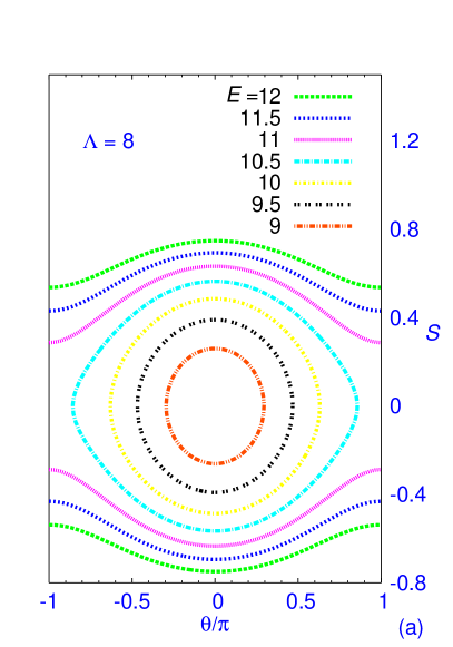
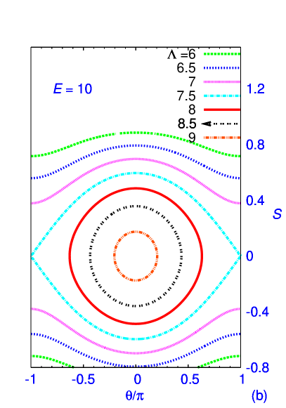
Figure 1: (Color online)Equi-energy phase contour plot of the unitary Fermi SF. (a) Contours of different energies for $\Lambda=8$. (b) Contours of $E=10$ for different values of $\Lambda$. Energy is in units of $2{\cal K}$.

As can be seen from Fig. 1, if we draw equi-energy contours of $H$ in the phase space of $(S,\theta)$, we can see two types of contours: those that form closed loop and those do not. The division of these two types of contours occurs at the critical energy (we take $2{\cal K}$ as the units for energy)

$$E_{\rm crit}=H(S=0,\theta=\pi)=\frac{6\Lambda}{5}+1\,.$$

If the system has energy $E<E_{\rm crit}$, its dynamics will follow the closed contours, and both $S$ and $\theta$ will oscillate in time. In particular, the population imbalance $S$ oscillates around 0 and the time averaged population imbalance vanishes. This corresponds to the AC Josephson regime. On the other hand, if the system has energy $E>E_{\rm crit}$, it will follow the open contours where $\theta$ will grow indefinitely and $S$ will oscillate around a non-zero value and will never cross the $S=0$ line. This corresponds to the self-trapping regime.

Given the initial values $S(0)$ and $\theta(0)$, the system moves on a contour of constant energy given by

$$E_{0} = \frac{3\Lambda}{5}\left[(1+S(0))^{5/3}+(1-S(0))^{5/3}\right]$$

$$\;\;-\sqrt{1-S(0)^{2}}\cos\theta(0)\,.$$

The condition for self-trapping

$$E_{0}>E_{\rm crit}=\frac{6\Lambda}{5}+1\,,$$

may be recast into the form

$$\Lambda>\Lambda_{c}=\frac{5}{3}\frac{1+\sqrt{1-S(0)^{2}}\,\cos\theta(0)}{(1+S(0))^{5/3}+(1-S(0))^{5/3}-2}\,.$$ (18)

In other words, within the two-mode model, the ratio of the nonlinear strength and the tunneling energy, $\Lambda$, determines whether the system should be self-trapped or not.

To determine the values of these quantities, we need to choose properly the spatial mode functions $\phi_{1,2}(x)$. A reasonable choice is given by trappingPRL ; I2M

$$\phi_{1,2}(x)=\frac{\phi_{+}(x)\pm\phi_{-}(x)}{\sqrt{2}}\,,$$

where the normalized wave functions $\phi_{\pm}(x)$ are the lowest-energy symmetric and antisymmetric stationary solutions to the time-independent DF equation:

$$\bar{\mu}_{\pm}\phi_{\pm}=\left[-\frac{1}{2}\frac{d^{2}}{dx^{2}}+U(x)+\frac{3\xi}{5}\left(\frac{N\lambda}{\pi}\right)^{2/3}|\phi_{\pm}|^{4/3}\right]\,\phi_{\pm}\,,$$

with chemical potential $\mu_{\pm}$.

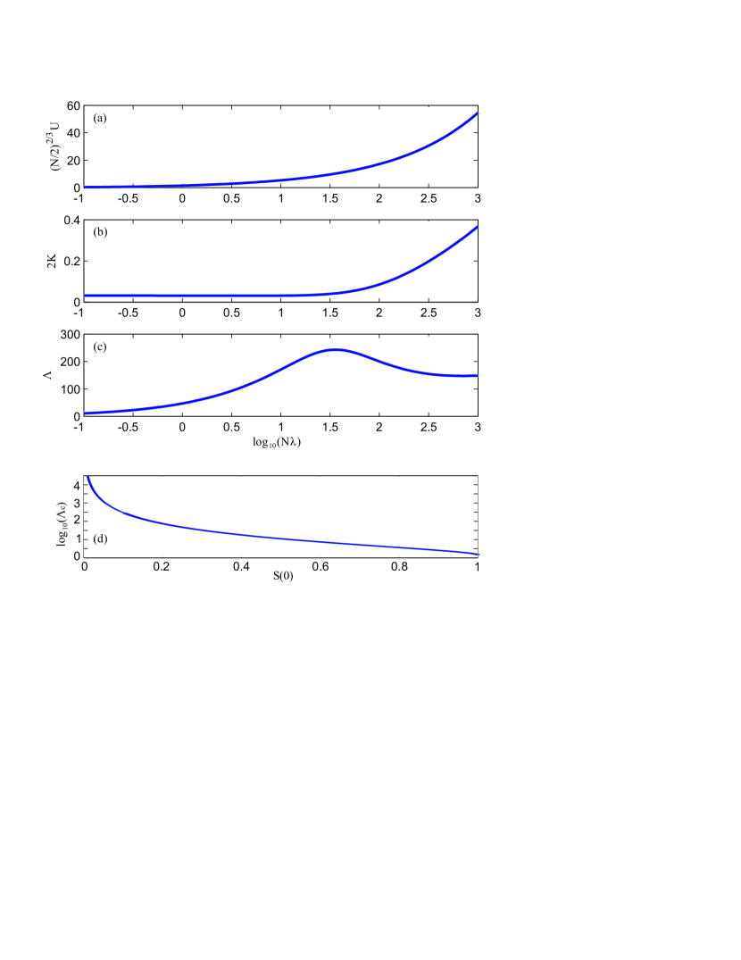
Figure 2: (a) Strength of nonlinearity $(N/2)^{3/2}U$, (b) tunneling energy $2{\cal K}$, and (c) their ratio $\Lambda$ (c) as functions of $N\lambda$ at unitarity. (d) The critical $\Lambda_{c}$ as function of $S(0)$ for $\theta(0)=0$ [see Eq. (18)].

In Figs. 2 (a), (b), and (c) we illustrate the nonlinear strength $(N/2)^{2/3}U$, tunneling energy $2{\cal K}$ and their ratio $\Lambda$ as functions of $N\lambda$, respectively. As $N\lambda$ increases, the strength of the (repulsive) nonlinearity increases. As a result, the $\phi_{1}$ and $\phi_{2}$ become widened and enjoy more overlap. This leads to an increased tunneling energy. However, the ratio of the nonlinear strength and the tunneling energy $\Lambda$ does not have a monotonic behavior as $N\lambda$ is increased. As shown in Fig. 2(c), $\Lambda$ initially increases for small $N\lambda$, reaches a peak and then decreases. In a recent study, Salasnich et al. newref used the local-density approximation on top of quantum Monte-Carlo data of Ref. the1 to explore the phase diagrams and find regimes of Josephson tunneling and of dynamical self-trapping of a 3D Fermi superfluid. In the two-mode approach reported in Ref. newref , a constant tunneling energy is arbitrarily chosen for the whole crossover regime. This is an inappropriate oversimplification. In Fig. 2(d), we show the critical value $\Lambda_{c}$ as a function of the initial population imbalance $S(0)$. One can see that as $S(0)$ increases, $\Lambda_{c}$ decreases rapidly.

The fact that $\Lambda$ is bounded from above even though the interaction strength can increase without bound has important consequences. For example, for certain initial conditions, self-trapping may only occur within an intermediate range of nonlinearity. Both too small and too large a nonlinearity will destroy self trapping. This statement is also true away from the unitarity, even in the BEC limit. Furthermore, for a sufficiently small $S(0)$, $\Lambda$ may never exceed the corresponding $\Lambda_{c}$. When this is the case, the system will always stay in the Josephson oscillation regime. For example, according to Fig. 2(d), $\Lambda_{c}\approx 300$ for $S(0)=0.1$. Fig. 2(c) shows that the system can therefore never reach the self-trapping regime if $S(0)$ equals 0.1 or smaller. This is consistent with our numerical results.

We want to remark that even though results obtained from the simple two-mode model may provide significant qualitative insights, they are not expected to be accurate quantitatively. Particularly for large nonlinearity, predictions from the two-mode model can deviate greatly from the numerical results I2M ; hanpu . The error mainly occurs in estimating the tunneling energy ${\cal K}$. The two-mode equations (12) and (13) are obtained by neglecting many terms involving overlap integrals of the mode functions $\phi_{1}$ and $\phi_{2}$, and hence in general greatly underestimates the tunneling energy, particularly for large nonlinearity when overlap between $\phi_{1}$ and $\phi_{2}$ can be significant. Furthermore, the two-mode approximation itself becomes questionable for large nonlinearity. When there is exchange of atoms between the two wells, the mode functions will change accordingly due to the modification of the nonlinear mean-field. Indeed, in our numerical calculations to be presented below, we observe that the spatial wave function of the system changes in time. In certain regimes, this change is significantly enough to invalidate the two mode model.

IV Numerical results

In this section we present an account of the numerical study of self-trapping and Josephson oscillation in a double-well potential by solving the full quasi-1D DF GP equation (9) valid for a cigar-shaped SF. The double-well potential is taken as

$$U(x)=x^{2}/2+Ae^{-\kappa x^{2}}.$$ (19)

We shall take the parameters $A$ and $\kappa$ of this double well similar to the ones employed in Ref. hanpu in a study of self-trapping with dipolar bosonic atoms.

To create an initial state with desired population imbalance for a given set of parameters $N\lambda$ and $a$, we search for the ground state of an asymmetric well comprised of an off-centered harmonic potential and the Gaussian barrier potential

$$U^{\prime}(x)=(x-x_{0})^{2}/2+Ae^{-\kappa x^{2}}.$$ (20)

The ground state of this asymmetric well is obtained by solving the time-independent version of the DF GP equation (9) using the imaginary time evolution method. The parameter $x_{0}$ in (20) is chosen so that the population imbalance

$$S(t)=(N_{1}(t)-N_{2}(t))/N\,,$$ (21)

has a fixed pre-determined initial value $S(0)$. Here $N_{1}(t)$ and $N_{2}(t)$ are the number of dimers in the first and the second well of the double-well potential. Experimentally, this is indeed the method used to generate the initial population imbalance GatiJPB2007 . We have also considered other forms of initial wave functions and found that the final results are qualitatively insensitive to the specific forms provided the initial population imbalance $S(0)$ is kept fixed at a small value. However, at a quantitative level the results could be sensitive to the form of the initial wave function. The sensitivity of the result to the initial wave form increases as $S(0)$ is increased. Moreover, the results are quite sensitive to the initial $S(0)$ employed.

Once the initial wave function is chosen, Equation (9) is solved numerically after discretization with the Crank-Nicolson scheme MA ; MA2 employing space and time steps 0.025 and 0.0002, respectively, using real-time propagation with the FORTRAN programs provided in Ref. MA . The results are also independently confirmed using a MATLAB code based on the split fast Fourier transform method.

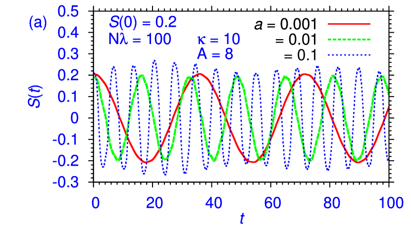
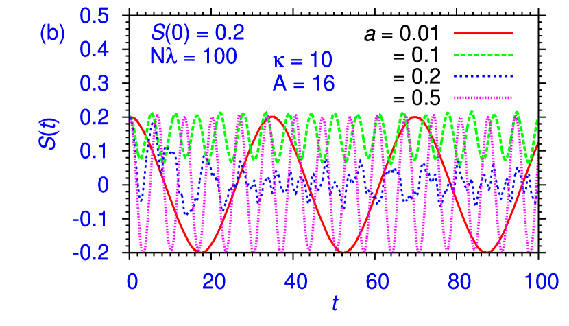
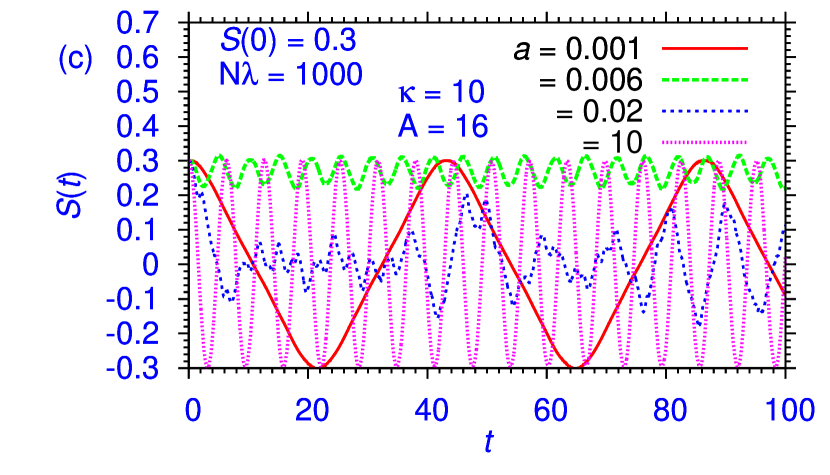
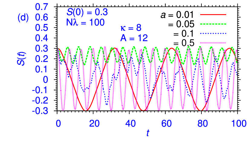
Figure 3: (Color online) Population imbalance $S(t)$ vs. $t$ dynamics with (a) $N\lambda=100,S(0)=0.2,\kappa=10,A=8$, (b) $N\lambda=100,S(0)=0.2,\kappa=10,A=16$, (c) $N\lambda=1000,S(0)=0.3,\kappa=10,A=16$, (d) $N\lambda=100,S(0)=0.3,\kappa=8,A=12$, for dimer-dimer scattering length $a$ varying over the BEC-unitarity crossover.

Now we present results of dynamical evolution of a Fermi SF, where we take $\xi=13.37$ in Eqs. (9) and (10). The numerical study of self-trapping and Josephson oscillation with the Fermi SF of dimers along the BEC-unitarity crossover reveals interesting features. To start the investigation of self-trapping we fix the trap parameters $A$ and $\kappa$ in Eqs. (19) and (20) at nontrivial values (a not too small value of $A$ and a not too large $\kappa$), which permit smooth and free Josephson oscillation in the BEC limit ($a=0$). Note that a very small value of $A$ and a very large value of $\kappa$ tend to reduce the double well (19) to a single well where there cannot be any self trapping and Josephson oscillation should appear for all values of $a$ and $N$. In order to have self trapping, $A$ cannot be too small and $\kappa$ cannot be too large. This is illustrated in Fig. 3 (a) for $A=8,\kappa=10,N\lambda=100,S(0)=0.2$ and for $a=0.1,0.01,$ and 0.001 where we plot $S(t)$ vs. $t$. There is no self trapping for a very small value of $S(0)(=0.1)$. The quantity $S(t)$ is experimentally measurable and $S(t)$ vs. $t$ dynamics provides information about self trapping and Josephson oscillation. From Fig. 3 (a) we find that there is Josephson oscillation for all values of $a$ and there is no sign of self trapping. (A nonzero time average $\langle S(t)\rangle$ ensures self trapping.) But a completely new scenario emerges as $A$ is increased to 16 from 8, as can be seen from Fig. 3 (b) where we show the $S(t)$ vs. $t$ dynamics for $a=0.01,0.1,0.2$ and 0.5. The plots for $a=0.01$ and 0.5 of Fig. 3 (b) are quite similar to the plots for $a=0.001$ and 0.1 of Fig. 3 (a) illustrating regular (periodic) Josephson oscillation with no sign of self trapping. But, for intermediate values 0.1 and 0.2 of $a$, self trapping and irregular (non-periodic) oscillation can be seen in Fig. 3 (b). In Figs. 3 (c) and (d) we illustrate two more cases of $S(t)$ vs. $t$ dynamics with a different value of $S(0)(=0.3)$ and different $N\lambda$ and trap parameters, respectively, where one can clearly find self trapping.

In the following, we discuss in detail the results for three initial population imbalance $S(0)=0.1$, 0.2 and 0.3, which are representative for a general case.

Population imbalance $S(0)=0.1:$ For this relatively small initial population imbalance, we found that for any values of $N\lambda$ and $a$, the system is always in the Josephson regime: the population imbalance $S(t)$ oscillates sinusoidally between $S(0)=-0.1$ and $S(0)=0.1$. The system never exhibits self-trapping. The frequency of oscillation increases as the strength of nonlinearity increases. Note that the strength of nonlinearity is increased by increasing either $N\lambda$ or $a$. However, the nonlinear interaction among dimers saturates as scattering length $a\to\infty$ at unitarity, it increases indefinitely with $N\lambda$. This result is consistent with our previous discussion of the two-mode model: For a sufficiently small $S(0)$, the required critical value of $\Lambda_{c}$ for self-trapping cannot be achieved by increasing the strength of the nonlinearity and the system stays in the Josephson regime for all values of $N\lambda$ and $a$.

Population imbalance $S(0)=0.2:$ The results for the $S(t)$ vs. $t$ dynamics for this initial population imbalance is illustrated in Figs. 3 (a) and (b) for fixed $N\lambda=100$ and various values of $a$ and two different traps as described earlier. In Fig. 3 (b), for a small scattering length of $a=0.01$ (solid line), Josephson oscillation is observed. When $a$ is increased to 0.1 (dashed line), self-trapping is clearly seen — $S(t)$ does not deviate from $S(0)$ too much and never crosses zero. With further increase of $a$ to a slightly larger value of 0.2 (dotted line), self-trapping is destroyed and $S(t)$ exhibits irregular oscillations around zero. Accompanied with this irregular population oscillation, the density profile $|\psi(x,t)|^{2}$ also develops complex and irregular structures. Remarkably, upon further increase of $a$, as the dot-dashed curve for $a=0.5$ shows, regular oscillation returns and the population dynamics once again exhibits sinusoidal Josephson oscillations.

Population imbalance $S(0)=0.3:$ Finally, let us discuss this relatively large initial population imbalance. If we use $N\lambda=100$ as we did above for $S(0)=0.2$, when $a$ is increased from zero to $\infty$, the system sequentially makes transitions from Josephson, to self-trapping and finally to irregular oscillation regimes. The Josephson oscillation is never recovered for $N\lambda=100$ for very large values of scattering length $a$ (results not shown here). In Fig. 3 (c) we plot the results for $S(t)$ vs. $t$ dynamics for $N\lambda=1000$. In this case, in addition to the three regimes just mentioned, for a sufficiently large $a{{(=10)}}$, Josephson oscillation is restored, just as in the case of $S(0)=0.2$ and $N\lambda=100$ discussed above. In Fig. Fig. 3 (d) we show another example of $S(t)$ vs. $t$ dynamics for a different trap, which is quite similar to that in Fig. 3 (c). We also did some calculation with larger $S(0)$ where a similar panorama emerges and we do not report the details here.

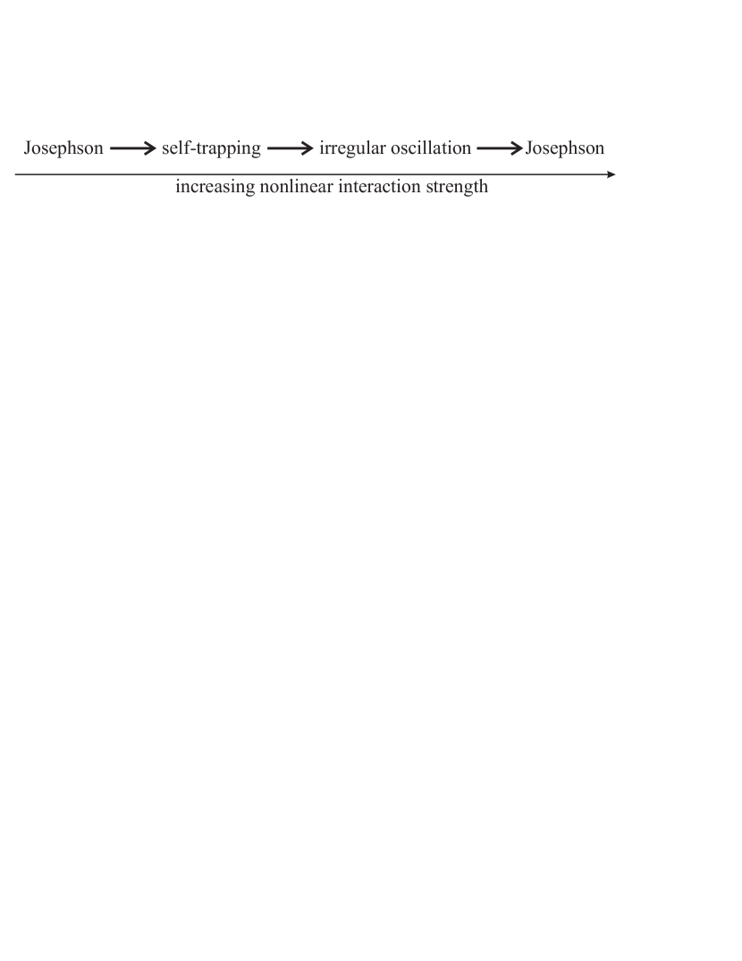
Figure 4: Different dynamical regimes of Fermi super-fluid in the BEC-unitary crossover.

To summarize the general characteristics of the population dynamics, we find that for any given initial population imbalance and for either sufficiently small or sufficiently large nonlinear interaction strength, the system is in the Josephson oscillation regime. For intermediate interaction strength, the system can make transition to self-trappping and irregular oscillation regimes as schematically shown in Fig. 4. The critical interaction strength at which the system makes the transition to self-trapping is sensitive to the initial population imbalance and increases sharply as $S(0)$ increases. (It is also sensitive to the parameters for the Gaussian barrier that creates the double-well potential.) It is possible that for a sufficiently small $S(0)$, the system always stays in the Josephson regime. The restoration of the Josephson oscillation at large interaction strength may seem surprising at first sight. However, one can understand it in the following intuitive way. For a sufficiently large interaction strength, the chemical potential is large and the effect of the Gaussian barrier becomes relatively unimportant. The wave functions on opposite sides of the barrier have sufficient overlap and hence the cloud tunnel back and forth without difficulty.

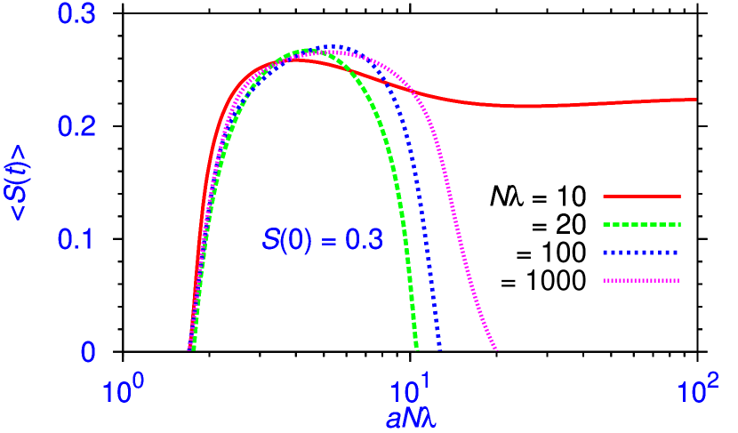
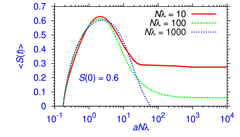
(a) (b)

Figure 5: (Color online) Time-averaged population imbalance $\langle S(t)\rangle$ vs. nonlinearity $aN\lambda$ for different $N\lambda$ for trap parameters $A=16,\kappa=10$ and (a) $S(0)=0.3$ and (b) $S(0)=0.6$. Different curves are generated by varying the scattering length $a$ across the BEC-unitarity crossover for $S(0)=0.3$ and 0.6, respectively, based on initial wave form (20).

The appearance of self-trapping is best illustrated through a study of the time-averaged population imbalance $\langle S(t)\rangle$ vs. nonlinearity $aN\lambda$ and we do that next. In Fig. 5 (a) we plot $\langle S(t)\rangle$ vs. $aN\lambda$ by varying the scattering length from 0 to $\infty$ for a fixed $N\lambda$ with trap parameters $A=16$ and $\kappa=10$. The initial population imbalance is chosen as $S(0)=0.3$. In Fig. 5 (a), with the increase of $aN\lambda$, self-trapping appears for $aN\lambda$ slightly greater than unity. With further increase of $aN\lambda$, self-trapping increases with an increase of $\langle S(t)\rangle$. For $N\lambda=10$, self trapping never disappears and continues even at unitarity. However, beyond $aN\lambda\approx 5$ self-trapping decreases with the increase of $aN\lambda$ for $N\lambda=20,100$ and 1000. For larger $N\lambda,$ $\langle S(t)\rangle$ eventually goes to zero as the nonlinear repulsion becomes too large to maintain all dimers in a single trap, except for $N\lambda=10$. In Fig. 5 (b) we exhibit a similar plot for $S(0)=0.6$ with trap parameters $A=16$ and $\kappa=10$.

Finally, to check the validity of the quasi-1D approximation, we performed full 3D numerical simulations based on Eqs. (5) and (6). The quasi-1D approximation should be valid when $\mu\ll\lambda\hbar\omega$. We have chosen different sets of parameters, some of which satisfy and the rest violate the quasi-1D condition. For parameters such that the quasi-1D condition is satisfied, we indeed find that our 3D numerical results are nearly identical to the 1D results presented here. For parameters that the quasi-1D condition is violated, the 3D results show deviations from the 1D ones. However, the qualitative features (i.e., the dependence of different dynamical regimes on the initial population imbalance and the strength of nonlinearity) presented in Figs. 3 and 5 remain valid. Specifically, we verified that the results reported in Figs. 3 remain essentially valid in the 3D model. This assures us of the reliability of the present study in 1D.

V Summary and Conclusion

To summarize, we have studied the dynamical properties of a Fermi SF confined in a double-well potential in the BEC-unitary crossover regime. To this purpose, we have developed a nonlinear Schödinger equation valid in the whole regime based on a density functional approach and on the equations of state from quantum Monte Carlo calculations. This equation is equivalent to the hydrodynamic equations with the quantum pressure term included. In the BEC side of the crossover, it describes accurately the equilibrium and low-energy dynamical properties of the Fermi SF. In particular, Josephson effect has been investigated using this method sala and the results have been shown to agree with those obtained from the microscopic approach by solving the Bogoliubov-de Gennes equations bdg . Compared with the latter, the great advantage of the current approach is its mathematical simplicity.

We have identified three dynamical regimes of the system: the Josephson regime, the self-trapping regime and the irregular oscillation regime. For a given initial population imbalance, these regimes are accessed according to the strength of nonlinearity as schematically shown in Fig. 4. The Josephson regime is always reached at either sufficiently small or sufficiently large interaction strength. For a small initial population imbalance, Josephson regime may be the only regime that the system can have access to. Note that the strength of nonlinearity can be increased by either increasing the number of dimers $N$ or the scattering length $a$. However, it saturates as $a$ tends to infinity while no saturation occurs for large $N$.

The quasi-1D model $-$ Eqs. (9) and (10) $-$ presented and used in the study of dynamical evolution of a Fermi SF in the BEC-unitarity crossover in this paper is also valid for an atomic BEC with a slightly modified value for the parameter $\xi$. Hence the present results for self-trapping of a Fermi SF in a double-well potential are also applicable for a repulsive atomic BEC when the atomic scattering length varies from 0 to $\infty$. However, in this case there could be practical difficulty with three-body loss in the experimental realization of the system for large scattering length.

We have also developed a simple analytical two-mode model, analogous to the much studied system of a BEC in a double-well potential. We show that the properties of the system can be described by a classical Hamiltonian with population imbalance and relative phase as a pair of conjugate variables. The great advantage of the two-mode model is its simplicity which makes analytical studies possible. The key parameters that characterize the two-mode model are the strength of nonlinearity and the tunneling energy. We calculated these parameters using the spatial mode function obtained by numerically solving the full time-independent nonlinear Schrödionger equation. From this calculation we show that the ratio of the interaction strength and the tunneling rate cannot increase indefinitely when the interaction strength increases. This explains the numerical observation that for sufficiently small initial population imbalance, the system may always stay in the Josephson regime. However, care must be taken when making quantitative comparisons with numerical results. In particular, for strong nonlinearity, the two-mode model can be even qualitative incorrect. For example, this model predicts the existence of the Josephson and the self-trapping regime, but not the irregular oscillation regime found in the numerical calculation, which occurs at relatively large nonlinearity and lies in the regime where the two-mode model is no longer valid.

- (1) L. Pitaevskii and S. Stringari, Bose-Einstein Condensation (Oxford University Press, Oxford, 2003); C. J. Pethick and H. Smith, Bose-Einstein Condensation in Dilute Gases (Cambridge University Press, Cambridge, England, 2002).
- (2) A. Görlitz et al., Phys. Rev. Lett. 87, 130402 (2001).
- (3) M. Albiez, R. Gati, J. Folling, S. Hunsmann, M. Cristiani, and M. K. Oberthaler, Phys. Rev. Lett. 95, 010402 (2005), R. Gati and M. K. Oberthaler, J. Phys. B 40, R61-R89 (2007).
- (4) A. Kastberg et al., Phys. Rev. Lett. 74, 1542 (1995).
- (5) G. Roati et al. Nature (London) 453, 891 (2008); S. K. Adhikari and L. Salasnich, Phys. Rev. A 80, 023606 (2009).
- (6) K. E. Strecker et al., Nature 417, 150 (2002); L. Khaykovich et al., Science 256, 1290 (2002).
- (7) B. Eiermann et al., Phys. Rev. Lett. 92, 230401 (2004); O. Morsch and M. Oberthaler, Rev. Mod. Phys. 78, 179 (2006).
- (8) B. P. Anderson et al., Phys. Rev. Lett. 86, 2926 (2001).
- (9) A. Smerzi, S. Fantoni, S. Giovanazzi, and S.R. Shenoy, Phys. Rev. Lett. 79, 4950 (1997); S. Raghavan, A. Smerzi, S. Fantoni, and S.R. Shenoy, Phys. Rev. A59, 620 (1999).
- (10) F. S. Cataliotti et al., Science 293, 843 (2001).
- (11) S. Levy, E. Lahoud, I. Shomroni, and J. Steinhauer, Nature 449, 579 (2007).
- (12) L. Morales-Molina and J. B. Gong, Phys. Rev. A 78, 041403(R) (2008).
- (13) E. A. Ostrovskaya, Y. S. Kivshar, M. Lisak, B. Hall, F. Cattani, and D. Anderson, Phys. Rev. A 61, 031601(R) (2000).
- (14) A. Trombettoni and A. Smerzi, Phys. Rev. Lett. 86, 2353 (2001).
- (15) J. Javanainen, Phys. Rev. Lett. 57, 3164 (1986); J. E. Williams, Phys. Rev. A 64, 013610 (2001); S. Giovanazzi et al., Phys. Rev. Lett. 84, 4521 (2000); I. Zapata et al., Phys. Rev. A 57, R28 (1998); S. K. Adhikari, Phys. Rev. A 72, 013619 (2005); Eur. Phys. J. D 25, 161 (2003).
- (16) S. Pereverzev et al., Nature 388, 449 (1997); S. Backhaus et al., Science 278, 1435 (1997).
- (17) K. Sukhatme et al., Nature 411, 280 (2001).
- (18) F. Ancilotto, L. Salasnich, and F. Toigo, Phys. Rev. A 79, 033627 (2009); L. Salasnich, F. Ancilotto, N. Manini, and F. Toigo, Laser Phys. 19, 636 (2009).
- (19) L. Pezzè et al., Phys. Rev. Lett. 93, 120401 (2004); S. K. Adhikari, Eur. Phys. J. D 47, 413 (2008).
- (20) M. Greiner et al., Nature (London) 426, 537 (2003); C. Chin et al., Science 305, 1128 (2004); C. A. Regal et al., Phys. Rev. Lett. 92, 040403 (2004); J. Kinast et al., ibid. 92, 150402 (2004); M. W. Zwierlein et al., ibid. 92, 120403 (2004); M. Bartenstein et al., ibid. 92, 203201 (2004); M. W. Zwierlein et al., Nature 435, 1047 (2005).
- (21) J. Kinast et al., Science 307, 1296 (2005); G. B. Partridge et al., ibid. 311, 503 (2006); T. Bourdel et al., Phys. Rev. Lett. 91, 020402 (2003); M. Bartenstein et al., ibid. 92, 120401 (2004).
- (22) S. Giorgini et al., Rev. Mod. Phys. 80, 1215 (2008).
- (23) A. Bulgac and G. F. Bertsch, Phys. Rev. Lett. 94, 070401 (2005); S. Stringari, ibid. 102, 110406 (2009); G. M. Bruun et al., ibid. 100, 240406 (2008);
- (24) E. P. Gross, Nuovo Cimento 20, 454 (1961); L. P. Pitaevskii, Zh. Eksp. Teor. Fiz. 40, 646 (1961) [Sov. Phys. JETP 13, 451 (1961)].
- (25) R. M. Dreizler and E. K. U. Gross, Density Funtional Theory (Springer-Verlag, Berlin, 1990).
- (26) S. K. Adhikari and L. Salasnich, Phys. Rev. A 78, 043616 (2008).
- (27) S. K. Adhikari and L. Salasnich, New J. Phys. 11, 023011 (2009).
- (28) D. Blume, J. von Stecher, and C. H. Greene, Phys. Rev. Lett. 99, 233201 (2007); J. von Stecher, C. H. Greene, and D. Blume, Phys. Rev. A 77, 043619 (2008); S. Y. Chang and G. F. Bertsch, Phys. Rev. A 76, 021603(R) (2007).
- (29) H. Heiselberg, Phys. Rev. A 63, 043606 (2001); G. A. Baker, Jr., Phys. Rev. C 60, 054311 (1999); Int. J. Mod. Phys. B 15, 1314 (2001).
- (30) G. E. Astrakharchik et al., Phys. Rev. Lett. 93, 200404 (2004); J. Carlson et al., ibid. 91, 050401 (2003).
- (31) J. R. Engelbrecht, M. Randeria, and C. A. R. S´a de Melo, Phys. Rev. B 55, 15153 (1997); S. Y. Chang et al., Phys. Rev. A 70, 043602 (2004).
- (32) M. E. Gehm et al., Phys. Rev. A 68, 011401(R) (2003); J. Kinast et al., Science 307, 1296 (2005); T. Bourdel et al., Phys. Rev. Lett. 91, 020402 (2003); M. Bartenstein et al., Phys. Rev. Lett. 92, 120401 (2004); G. B. Partridge et al., Science 311, 503 (2006); J. T. Stewart et al., Phys. Rev. Lett. 97, 220406 (2006).
- (33) S. Cowell et al., Phys. Rev. Lett. 88, 210403 (2002).
- (34) D. S. Petrov et al., Phys. Rev. Lett. 93, 090404 (2004).
- (35) J. K. Nilsen, J. Mur-Petit, M. Guilleumas, M. Hjorth-Jensen, and A. Polls, Phys. Rev. A 71, 053610 (2005).
- (36) T. D. Lee and C. N. Yang, Phys. Rev. 105, 1119 (1957); T.D. Lee, K. Huang and C. N. Yang, Phys. Rev. 106, 1135 (1957).
- (37) T. T. Wu, Phys. Rev. 115, 1390 (1959); E. Bratten and A. Nieto, Eur. Phys. J. B 11, 143 (1999).
- (38) W. Lenz, Z. Phys. 56, 778 (1929).
- (39) A. Fabrocini and A. Polls, Phys. Rev. A 60, 2319 (1999); 64, 063610 (2001).
- (40) S. K. Adhikari and L. Salasnich, Phys. Rev. A 77, 033618 (2008).
- (41) S. K. Adhikari, Phys. Rev. A 79, 023611 (2009); Laser Phys. Lett. 6, 901 (2009).
- (42) S. K. Adhikari, unpublished (2009).
- (43) D. Blume and C. H. Greene, Phys. Rev. A 63, 063601 (2001).
- (44) J. von Stecher, C. H. Greene, and D. Blume, Phys. Rev. A 76, 053613 (2007).
- (45) N. Manini and L. Salasnich, Phys. Rev. A 71, 033625 (2005); Y.E. Kim and A.L. Zubarev, Phys. Rev. A 70, 033612 (2004); S. K. Adhikari, Phys. Rev. A 77, 045602 (2008).
- (46) L. Salasnich, A. Parola, and L. Reatto, Phys. Rev. A 65, 043614 (2002); A. Muñoz Mateo and V. Delgado, Phys. Rev. A 77, 013617 (2008); C. A. G. Buitrago and S. K. Adhikari, J. Phys. B, 42, 215306 (2009).
- (47) L. Salasnich, N. Manini and F. Toigo, Phys. Rev. A 77, 043609 (2008).
- (48) D. Ananikian and T. Bergeman, Phys. Rev. A 73, 013604 (2006).
- (49) Bo Xiong, J. Gong, Han Pu, W. Bao, and B. Li, Phys. Rev. A 79, 013626 (2009).
- (50) P. Muruganandam and S. K. Adhikari, Comput. Phys. Commun. 180, 1888 (2009).
- (51) P. Muruganandam and S. K. Adhikari, J. Phys. B 36, 2501 (2003); S. K. Adhikari and P. Muruganandam, J. Phys. B 35, 2831 (2002).
- (52) A. Spuntarelli, P. Pieri, and G. C. Strinati, Phys. Rev. Lett. 99, 040401 (2007).