Classical Analogue of the Ionic Hubbard Model

Abstract

In our earlier work [M. Hafez, et al., Phys. Lett. A 373 (2009) 4479] we employed the flow equation method to obtain a classical effective model from a quantum mechanical parent Hamiltonian called, the ionic Hubbard model (IHM). The classical ionic Hubbard model (CIHM) obtained in this way contains solely Fermionic occupation numbers of two species corresponding to particles with $\uparrow$ and $\downarrow$ spin, respectively. In this paper, we employ the transfer matrix method to analytically solve the CIHM at finite temperature in one dimension. In the limit of zero temperature, we find two insulating phases at large and small Coulomb interaction strength, $U$, mediated with a gap-less metallic phase, resulting in two continuous metal-insulator transitions. Our results are further supported with Monte Carlo simulations.

I Introduction

To understand the magnetism and magnetic phenomena, one of the basic interactions is the exchange mechanism which is deeply rooted in Coulomb interactions and quantum mechanical indistinguishability. Therefore a fair understanding of the magnetic behavior of materials is not possible without investigating appropriate quantum spin models. Introducing uni-axial anisotropy to the Heisenberg model amounts to suppression of transverse quantum fluctuations ($S^{+}S^{-}+S^{-}S^{+}$), leading to the so called Ising model Newell . The resulting Ising Hamiltonian turns out to contain the basic magnetic phases of the original Heisenberg model, namely ferromagnetism, and antiferromagnetism Feynman . Although many of the interesting possible aspects such as spin liquid phases, spin-wave excitations, etc. Fradkin can not be captured by the Ising model. Classical Ising model has the merit of being much simpler to solve, and admits analytical Newell ; Onsager and graphical solutions  Feynman in various geometries JafariIJMP in one and two dimensions which is lacking in the original quantum Heisenberg model.

Dielectric properties are among the most important properties characterizing materials. The question can be asked here, is there any Ising-like model that can provide basic informations about their phase diagram, and at the same time being simple enough to allow for analytical solutions? We have taken the example of the (IHM) Nagaosa ; Egami . This model was introduced to study the neutral-to-ionic transition in organic compounds, as well as, understanding the role of strong electronic correlations in the dielectric properties of metal oxides Egami ; HafezCUT . This model is as follows:

$$H = -t\sum_{i\sigma}(c^{{\dagger}}_{i\sigma}c_{i+1,\sigma}+h.c.)+U\sum_{i}c^{{\dagger}}_{i\uparrow}c^{{\dagger}}_{i\downarrow}c_{i\downarrow}c_{i\uparrow}$$ (1)

$$+\frac{\Delta}{2}\sum_{i\sigma}(-1)^{i}c^{{\dagger}}_{i\sigma}c_{i\sigma},$$

where $c_{i\sigma}$ ($c^{{\dagger}}_{i\sigma}$) is the usual annihilation (creation) operator at site $i$ with spin $\sigma$. $U$ is the on-site Coulomb interaction parameter, and $\Delta$ denotes a one-body staggered ionic potential. The kinetic energy scale is given by the real hopping amplitude $t$ which prefers to gain kinetic energy by spreading the wave-function over the whole system, leading to quantum fluctuation of the charge density. The zero temperature phase diagram of this model contains Mott and band insulating states when the energy scales corresponding to $U$ or $\Delta$ dominate, respectively HafezCUT . When these two scales become of the same order of magnitude, the nature of intermediate phase still remains controversial. Some authors argue that the intermediate state is a spontaneously broken symmetry phase SBSP , while some others argue that the phase in between is metallic Nagaosa ; Bouadim2007 ; HafezCUT ; Metals . In our previous investigation HafezCUT we employed the method of flow equations for the quantum Hamiltonian (1) to obtain an effective Hamiltonian in which the hopping $t$ term is renormalized to zero, producing a new nearest neighbor Coulomb attraction. The resulting classical Hamiltonian is of the following lattice gas form:

$$\tilde{H}=\frac{\widetilde{\Delta}}{2}\sum_{i\sigma}(-1)^{i}n_{i\sigma}+\widetilde{U}\sum_{i}n_{i\uparrow}n_{i\downarrow}+\widetilde{V}\sum_{i\sigma,\sigma^{\prime}}n_{i\sigma}n_{i\sigma^{\prime}},$$ (2)

where the renormalized parameters $\tilde{\Delta},\tilde{U},\tilde{V}$ have closed form expressions in terms of the bare parameters $U,\Delta$ HafezCUT . We take the kinetic energy scale $t$ as the unit of energy.

By calculating the spin and charge gaps, we showed that this simple classical model is capable of capturing the physics of a metallic state sandwiched between two distinct insulating phases at zero temperature as one increases $U$ for a fixed value of $\Delta$ HafezCUT . Here $n_{i\sigma}$ contains two species (or colors) corresponding to $\sigma=\uparrow,\downarrow$, respectively. Since $n_{\sigma}$ for each ”color” $\sigma$ is either $0$ or $1$, it is an Ising-like variable. Therefore our effective CIHM Hamiltonian can be thought of, as two inter-penetrating Ising models on a lattice. Being a natural extension of two species lattice gas model, allows for analytical solution in one spatial dimensions (1D). Here we can employ the transfer matrix method, constructed in terms of $3\times 3$ matrices to calculate the thermodynamic properties of this model at finite temperatures. At high temperatures where the thermal fluctuations wash out the quantum effects, we expect the results of our calculations to be a good description of the class of materials modeled in terms of IHM. Also a novel graphical solution in 2D similar to Feynman’s construction can be worked out JafariUnpublished .

The paper is organized as follows: In the next section we calculate the grand canonical potential for this model in one dimension and discuss the particle density and ionicity in various fillings. It is followed by a section focused on half-filling situation, and calculate the specific heat, compressibility and ionicity to assess the nature of the phases in the parameter space of $U,T$. Throughout the paper we have fixed the value of $\Delta=20$ HafezCUT . The final section is devoted to summary and discussion.

II Grand Potential

In this section we calculate the grand canonical potential that can be derived from the grand partition function (GPF) which is defined as follows:

$$Z(T,\mu,L)=\sum_{\{n_{i\sigma}\}}e^{-\beta\big{(}E(\{n_{i\sigma}\})-\mu N(\{n_{i\sigma}\})\big{)}},$$ (3)

where $T$ is Temperature, $L$ is lattice size, and $\mu$ is chemical potential. The $\{n_{i\sigma}\}$ denotes all possible configurations of the occupation numbers, which must be summed over. $N(\{n_{i\sigma}\})=\sum_{i\sigma}n_{i\sigma}$ is the number of particle and $E(\{n_{i\sigma}\})$ is the energy that is defined by the model Hamiltonian Eq. (2).

The summation in Eq. (3) can be calculated analytically as follows. The values of $n_{i\sigma}$ are only zero and one, which is the Fermionic memory left in the commuting variables $n_{i\sigma}$. Hence $n_{i\sigma}^{2}=n_{i\sigma}$, and the second term in Eq. (2) becomes:

$$\sum_{i}n_{i\uparrow}n_{i\downarrow}=\frac{1}{2}\sum_{i}(n_{i\uparrow}+n_{i\downarrow})[(n_{i\uparrow}+n_{i\downarrow})-1].$$ (4)

The GPF becomes,

$$Z(T,\mu,L)=\sum_{\{n_{i\sigma}\}}\exp\bigg{\{}-\beta\Big{[}\sum_{i\sigma}\big{(}(-1)^{i}\frac{\widetilde{\Delta}}{2}-\mu\big{)}n_{i\sigma}$$ (5)

$$+ \frac{\widetilde{U}}{2}\sum_{i\sigma,\beta}n_{i\sigma}(n_{i\beta}-\frac{1}{2})+\widetilde{V}\sum_{i\sigma,\beta}n_{i\sigma}n_{i\beta}\Big{]}\bigg{\}}.$$

As can be seen at the Hamiltonian level, only the spin-summed occupations appear and therefore this classical model does not contain spin-polarized (magnetic) solutions. So we change the summation variable from $n_{i\uparrow}$ and $n_{i\downarrow}$ to $n_{i}=n_{i\uparrow}+n_{i\downarrow}$ that has three possible values 0,1,2. Therefore we have:

$$Z=\sum_{\{n_{i}\}}\exp\bigg{\{} - \beta\sum_{i}\Big{[}\big{(}(-1)^{i}\frac{\widetilde{\Delta}}{2}-\mu\big{)}n_{i}+\frac{\widetilde{U}}{2}n_{i}(n_{i}-1)$$ (6)

$$+ \widetilde{V}n_{i}n_{i+1}\Big{]}\bigg{\}}\prod_{i=1}^{L}(1+\delta_{n_{i},1}),$$

where the coefficient $\prod_{i=1}^{L}(1+\delta_{n_{i},1})$ takes into account the two-fold degeneracy for $n_{i}=1$ in Eq. (5), which corresponds to either $n_{i\uparrow}=1$, $n_{i\downarrow}=0$, or $n_{i\uparrow}=0$, $n_{i\downarrow}=1$. Eq. (6) can be written in a more symmetric form,

$$Z = \sum_{\{n_{i}\}}\prod_{i=1}^{L}(1+\delta_{n_{i},1})^{\frac{1}{2}}(1+\delta_{n_{i+1},1})^{\frac{1}{2}}\exp\bigg{\{}-\beta\Big{[}$$ (7)

$$+ (-1)^{i}\frac{\widetilde{\Delta}}{4}(n_{i}-n_{i+1})-\frac{\mu}{2}(n_{i}+n_{i+1})$$

$$+ \frac{\widetilde{U}}{4}\big{(}n_{i}(n_{i}-1)+n_{i+1}(n_{i+1}-1)\big{)}+\widetilde{V}n_{i}n_{i+1}\Big{]}\bigg{\}},$$

where $L$ is assumed to be even and the periodic boundary conditions, $n_{L+1}=n_{1}$ is implied. Defining the matrix elements of the transfer matrix $M_{n_{1},n_{2}}$ by,

$$M_{n_{1},n_{2}} \equiv (1+\delta_{n_{1},1})^{\frac{1}{2}}(1+\delta_{n_{2},1})^{\frac{1}{2}}\exp\bigg{\{}-\beta\Big{[}$$ (8)

$$+ \frac{\widetilde{\Delta}}{4}(n_{1}-n_{2})-\frac{\mu}{2}(n_{1}+n_{2})$$

$$+ \frac{\widetilde{U}}{4}\big{(}n_{1}(n_{1}-1)+n_{2}(n_{2}-1)\big{)}+\widetilde{V}n_{1}n_{2}\Big{]}\bigg{\}},$$

Eq. (7) can be written as:

$$Z = \sum_{n_{1}=0}^{2}\cdots\sum_{n_{L}=0}^{2}M_{n_{2},n_{1}}M_{n_{2},n_{3}}\cdots M_{n_{L},n_{L-1}}M_{n_{L},n_{1}}$$ (9)

$$= \sum_{n_{1}=0}^{2}\cdots\sum_{n_{L}=0}^{2}M_{n_{1},n_{2}}^{t}M_{n_{2},n_{3}}\cdots M_{n_{L-1},n_{L}}^{t}M_{n_{L},n_{1}}$$

$$= \mbox{Tr}(M^{t}M)^{\frac{L}{2}},$$

where $M^{t}$ is the transpose of $M$, $M_{n_{2},n_{1}}\equiv(M^{t})_{n_{1},n_{2}}$. Then the partition becomes:

$$Z=\lambda_{1}^{\frac{L}{2}}+\lambda_{2}^{\frac{L}{2}}+\lambda_{3}^{\frac{L}{2}},$$ (10)

where $\lambda_{1}$, $\lambda_{2}$, and $\lambda_{3}$ are the eigenvalues of $M^{t}M$. In the thermodynamic limit where $L$ is very large, the grand potential per site becomes:

$$\phi=-\frac{T}{2}\ln\lambda_{max}.$$ (11)

Here $\lambda_{max}$ is the maximum eigenvalue. Hence to obtain the grand potential one needs to calculate the eigenvalues of $M^{t}M$. Later on, when we discuss the ionicity, we will in addition need the eigenvectors of $M^{t}M$. The eigenvalues of $M^{t}M$ are solutions to the third order equation,

$$\lambda^{3}+a_{2}\lambda^{2}+a_{1}\lambda+a_{0}=0,$$ (12)

with $a_{2}$, $a_{1}$, and $a_{0}$ given in the appendix. Through the paper we will report the numerical plots for $\Delta=20$ in units in which $t=1$. For this value of $\Delta$, there would be no level-crossing among the eigenvalues $\lambda$ of the matrix $M^{t}M$ when one varies $\mu$, $T$, and $U$, as expected from Perron’s theorem Goldenfeld .

Figure 1: Particle density $n$, versus chemical potential $\mu$ for $U=10$, $\Delta=20$ and different temperatures. Three plateaus at $n=0.5,1,1.5$ correspond to quarter-,half- and three quarter-fillings. For lower temperature, the variations of the density as a function of $\mu$ is very slow over the plateaus, which is clear signature of a gap in the spectrum at these commensurate fillings. By increasing the temperature, plateaus get rounder, which indicate the thermal energy starts to overcome the gaps. The inset magnifies the ”isosbestic” behavior at $n=1$ plateau.

From the partition function, one can in principle calculate various averages of the form $\langle n_{i\sigma}n_{j\sigma^{\prime}}...\rangle$. The simplest of these averages are the average particle density $n\equiv\langle n_{2i+1}+n_{2i}\rangle/2$ (symmetric combination), and the ionicity $I\equiv\langle n_{2i+1}-n_{2i}\rangle/2$ (antisymmetric combination) which contain important information about the nature of the thermodynamic phases of the model. In the following we calculate these averages as a function of $\mu$.

II.1 Particle Density

Once the grand potential $\phi$ is known, one can derive many other thermodynamic quantities. The particle density, $n$, can be calculated as,

$$n=-\frac{\partial\phi}{\partial\mu}\Big{|}_{T}.$$ (13)

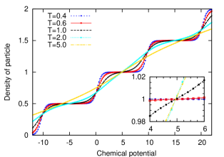
In Fig. 1, the particle density versus $\mu$ has been plotted for different values of $T$. In this figure the value of $U$ is fixed to be $U=10$. This value of $U$ corresponds to a band insulating regime at zero temperature HafezCUT . As can be seen in the figure, apart from trivial cases of the empty ($n=0$) and the fully-filled ($n=2$) lattice, there are three plateaus. The first one corresponds to the half-filling $n=1$ (i.e. one particle per lattice site), and two others correspond to commensurate fillings, $n=0.5$ (quarter-filling), $n=1.5$ (three-quarter-filling) which is quite similar to the plateaus of the parent ionic Hubbard model Bouadim2007 . Indeed the $n=0.5$ and $n=1.5$ are related by a particle-hole transformation. Therefore in what follows, we focus on $n=0.5,1$. With increasing the temperature, the plateaus get more and more rounded. The value of chemical potential corresponding to the half-filling is independent of temperature, as can be seen in Fig. 1. The inset plot indicates this point more transparently. This ”isosbestic” behavior is observed for all values of values of $10<U<40$.

Figure 2: Particle density $n$, versus chemical potential $\mu$ for constant $T=0.4,~{}\Delta=20$ and different values of $U$. As can be seen in general again there are three plateaus corresponding to $n=0.5,1,1.5$. However, for intermediate values of $U$, the plateau at half-filling has disappeared.

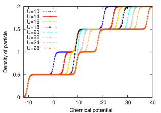
In Fig. 2, we have plotted the particle density as a function of chemical potential $\mu$ at a constant (low) temperature $T=0.4$, for different values of $U$. As can be seen in the figure, increasing $U$, causes the $n=0.5,1.5$ plateaus which are particle-hole counterpart of each other, get wider. However the plateau at $n=1.0$ gets narrower and finally vanishes around $U=20$, resulting in a gap-less phase at half-filling. Upon further increasing $U$, the half-filling plateau is recovered, and gets wider, indicating the emergence of a growing new gap in the system, which is reminiscent of the Mott insulating behavior. To identify the nature of gap at $n=0.5,1.5$ one needs to calculate the ionicity, which provides information about how the unit cell is being filled. This will be done in the sequel.

For later reference, we report the value of chemical potential corresponding to half-filling, which by examining the numerical plots turns out to be:

$$\mu(T,U,n=1)=0.495U.$$ (14)

The temperature range at which the above relation is valid, is roughly $0.1\lesssim T$. For temperatures outside this range, there will be deviations from the above rule of thumb relation.

II.2 Ionicity

Figure 3: The ionicity per site as a function of chemical potential for various temperatures at $U=10$. Three plateaus around $\mu\approx-5,5,15$ correspond to 1/4,1/2,3/4 filling.

If $A,B$ denote the sublattice of odd and even sites, respectively, then $N_{A}$ and $N_{B}$ are defined as:

$$N_{A} = \sum_{i\in\mbox{odd}}\langle n_{i}\rangle,$$ (15)

$$N_{B} = \sum_{i\in\mbox{even}}\langle n_{i}\rangle,$$ (16)

the ionicity per site becomes $I=(N_{A}-N_{B})/L$, where $n_{i}=n_{i\uparrow}+n_{i\downarrow}$, and $L$ is the total number of lattice sites. This quantity can also be calculated analytically with the aid of transfer matrices. In the grand canonical ensemble $\langle n_{j}\rangle$ is given by:

$$\langle n_{j}\rangle=\frac{1}{Z}\sum_{\{n_{i\sigma}\}}n_{j}e^{-\beta\big{(}E(\{n_{i\sigma}\})-\mu N(\{n_{i\sigma}\})\big{)}}.$$ (17)

Depending on whether $j$ is odd or even, similar to calculations for grand partition function, we obtain:

$$\langle n_{j}\rangle = \frac{1}{Z}\mbox{Tr}\left(N(M^{t}M)^{\frac{L}{2}}\right),~{}~{}~{}~{}~{}~{}~{}~{}\mbox{for odd }j$$ (18)

$$= \frac{1}{Z}\mbox{Tr}\left(N(MM^{t})^{\frac{L}{2}}\right),~{}~{}~{}~{}~{}~{}~{}~{}\mbox{for even }j$$ (19)

where $N$ is the following $3\times 3$ matrix:

$$N_{n_{1},n_{2}}=n_{1}\delta_{n_{1},n_{2}}.$$ (20)

Figure 4: Ionicity per site as a function of $\mu$ and constant temperature $T=0.4$, for various values of $U$. Three plateaus correspond to 1/4,1/2,3/4 filling, respectively. Note that the center of the half-filling plateau is at $\mu=U/2$.

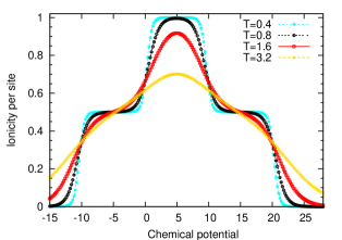
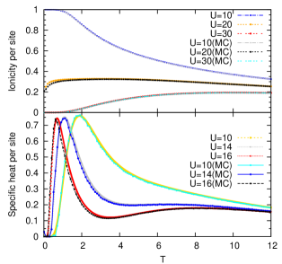
In Fig. 3, we have plotted the ionicity per site as a function of $\mu$ for various temperatures at a fixed value of $U=10$. For this value of $U$, at zero temperature one would expect a band insulator at half-filling, where A-sublattice (with on-site energy $-\Delta/2$) are doubly occupied. Let us focus around $\mu=-5$ which corresponds to quarter filling (c.f. Fig. 1). The value of $I=0.5$ for $\mu\approx-5$ in Fig. 3 shows that the only electron of each unit cell belongs to A-sublattice, which represents a charge density wave insulator.

As we increase $\mu$ from $\approx-5$, the ionicity increases, which indicates that sublattice A continues to be filled. When $\mu\approx 5$, one approaches the half-filling (Fig. 1), where at lower temperatures the A-sublattice is totally occupied, hence $I\approx 1$. As can be seen in Fig. 3, this saturation value is decreased as the temperature is increased. This reduction in the ionicity, indicates that the particles are bing thermally excited across the band gap. Further increasing of the chemical potential, one reaches the plateau around $\mu\approx 15$ of Fig. 3 (c.f. Fig. 1). The decrease in the ionicity indicates that the added particles essentially start to occupy the B-sublattice. The symmetry of Fig. 3 around $n=1$, is due to the apparent particle-hole symmetry of the Hamiltonian.

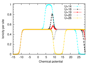
In Fig. 4 we plot the ionicity per site at the constant temperature $T=0.4$ and different values of $U$ indicated in the legend. Again there are three plateaus corresponding to 1/4,1/2 and 3/4-filling, respectively. This figure indicates that the center of the half-filling plateau is at $\mu_{1/2}=U/2$. This can be understood as a Hartree like energy for the Hubbard model. Now concentrating around half-filling in this figure, for small values of $U$, the ionicity reaches $1$, which indicates a complete electric polarization of the unit cell, and hence we have a band insulator. For intermediate values of $U$, the maximum value of ionicity does not reach $1$, which shows some of the added particles start to occupy the B-sublattice. Also note that for the intermediate values of $U$ the half-filling plateau starts to disappear, i.e. the emergence of a metallic behavior. For large values of $U$, the half-filling plateau is restored, but at zero ionicity. Therefore we have an insulator with unpolarized unit cell. Such an insulating state can be thought of as classical counterpart of the Mott insulating state.

III Half-filling

As we saw in Fig. 2, for $n=0.5,1.5$ the $U,\Delta$ energy scales cooperate with each other, to give rise to a charge density wave insulating ground state. Rather at $n=1.0$, these two energy scales compete against each other to destroy the insulating behavior for intermediate $U$ ($\sim\Delta$), giving rise to a richer phase diagram. Therefore in this section we focus at half-filling and calculate the specific heat, compressibility, and ionicity. Before doing so, we compare some physical quantities evaluated by a fully numerical Monte Carlo simulation, with our exact transfer matrix results. In Fig. 5, ionicity and specific heat per site are plotted at half-filling and show a good agreement between analytical and numerical results. This ensures that both Monte Carlo and analytic results are reliable.

Figure 5: Ionicity and specific heat per site at half-filling from transfer matrix and Monte Carlo (MC) methods. To stay in the range of validity of Eq. (14), transfer matrix results are plotted for $T\geq 0.1$. Monte Carlo results are obtained for $L=500$ sites. As stated earlier, we are working at constant $\Delta=20$.

Now let us proceed with the calculation of various thermodynamic quantities. For the fixed value of $\Delta=20$, we have two ways to plot thermodynamic quantities. First way is to plot them as a function of temperature $T$, at some selected values of $U$. These results indicate that in the present one dimensional model, there will be no finite temperature phase transition. This is obviously due to the analytic behavior of the partition function as a function of $T$. The second way is to plot them as a function of $U$, for some selected temperatures. This second way of presenting the data, reveals that as one lowers the temperature, there will be sharper features as a function of $U$, indicating the zero temperature phase transition. Our calculations are based on Eqs. (11,14). For very low temperatures, where the validity of Eq. (14), might be questioned, we employ Monte Carlo simulation data.

III.1 Specific heat

Figure 6: Specific heat per site versus $T$ at $\Delta=20$ for different values of $U$. For small values of $U$ there is a single peak, which becomes a peak-dip-hump in intermediate $U$, and finally the peak merges into the hump at large $U$. For $U=20$, both analytic and Monte Carlo results are reported . MC results are for $L=500$ sites.

Specific heat per site can be calculated as:

$$c_{L}=T\frac{\partial s}{\partial T},$$ (21)

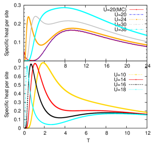
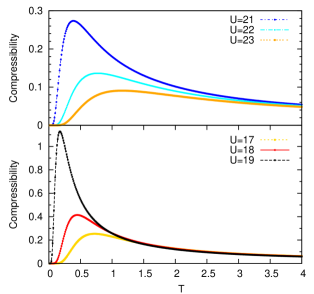
where $s$ is entropy per site at half-filling that can be derived from the grand potential. Figure 6 shows the specific heat versus $T$ for various values of $U$. As can be seen in Fig. 6 for values of $U\leq 14$, there is a single peak in the $c_{L}$. For $14<U<38$ a peak-dip-hump structure can be observed. For $U>20$ the hump is quite clear, while for $U<20$, it can be interpreted as a precursor to the hump. For $38\leq U$, the peak merges into the hump structure. In terms of the parent quantum Hamiltonian, such hump structure indicates incoherent excitations. For $U=20$, Eq. (14) is not reliable at very low temperatures. Therefore we report Monte Carlo simulation results which indicates a very sharp peak at $T\approx 0$. As $U$ moves towards $\approx 20$ from both sides (lower and upper panels), the peak gets sharper and moves towards lower temperatures. This indicates that in $T\to 0$ limit one expects a transition between gaped and gap-less states.

Figure 7: Estimate of gap using two-state model as a function of $U$ at $\Delta=20$.

This behavior can be simply understood in terms of a two-state model with level spacing $\delta$, whose specific heat is given by

$$c_{L}=k_{B}\left(x^{2}\frac{{\rm e}^{x}}{(1+{\rm e}^{x})^{2}}\right),$$ (22)

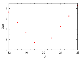
where $x=\delta/(k_{B}T)$. Behavior of Eq. (22) for $x\gg 1$ is like $\sim x^{2}{\rm e}^{-x}$, while for $x\ll 1$ it vanishes as $\sim x^{2}$. For the intermediate region a Schottky peak around $x_{\rm peak}\sim 1$ ($\delta\sim k_{B}T$) arises in the specific heat. Fitting the specific data to Eq. (22), in Fig. 7 we have plotted the estimated gap versus $U$, which indicates two gaped phases. According to the above two-state formula, this peak corresponds to $\delta/k_{B}T\sim 1$, from which a gap of $\delta\sim 10^{-2}$ can be estimated. If we extrapolate the estimated gap for $18<U<22$, zero gap region is expected to occur for $U_{c_{1}}=19.30\lesssim U\lesssim U_{c_{2}}=19.75$ which is compatible with our previous work HafezCUT .

Figure 8: Specific heat per site versus $U$ for different values of $T$.

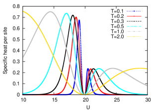
Now let us look at the specific heat data from a different angle. In Fig. 8 we plot the specific heat versus $U$ for different values of temperatures. As can be seen, there are two peak structures at all temperatures, which get sharper and by lowering the temperature, they tend to accumulate around $U\approx 20$. Extrapolating the trend of this double-peak structure to the limit of $T\to 0$, suggests two phase transitions at $U_{c1}$ and $U_{c2}$ HafezCUT , compatible with the behavior of the vanishing gap region in Fig. 7. The characteristic quadratic behavior around $U\approx 20$ seen in Fig. 8, which according to the two-state model is expected to be like $c_{L}\propto(\delta/T)^{2}$, indicates two continuous metal-insulator transitions, with $\delta\sim|U-U_{c_{i}}|$, $i=1,2$.

III.2 Compressibility

Another quantity that can be treated in our consideration CIHM is the compressibility which is given by:

$$\kappa=\frac{1}{n^{2}}\frac{\partial n}{\partial\mu}\Big{|}_{T},$$ (23)

where $n=N/L$ is the density of particles per site.

Figure 9: Compressibility versus $T$ for different values of $U$.

In Fig. 9 we plot the compressibility as a function of $T$ for different values of $U$. Zero compressibility is a characteristic of gaped states. As can be seen in this figure for small value of $U$ the range of temperatures at which the compressibility is close to zero is substantial, which means that the gap is so large that up to such temperature the insulating behavior is still manifest. By increasing $U$, this temperature range shrinks and becomes smaller and smaller, until around $U=20$, it extrapolates to zero. Increasing $U$ beyond $20$, again recovers a finite temperature range in which the compressibility is zero. This behavior confirms that a gap-less state is sandwiched between two gaped states.

To see the above statement more clearly, in Fig. 10 we plot compressibility as a function of $U$ for selected temperatures.

Figure 10: Compressibility versus $U$ for different values of temperature.

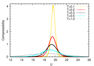
As can be seen in this figure, there is a region with non-zero compressibility, which characterizes a gap-less phase. Outside this region, the compressibility decays to zero. By decreasing $T$, the width of the compressibility peak becomes smaller and while the height of the peak diverges as $T\to 0$; a typical characteristic of a continuous phase transition. This confirms the existence of a metallic phase at zero temperature HafezCUT . The effect of thermal fluctuations is to smear the edges of metallic region. This is quite intuitive, as for values of $U$ near the zero temperature boundary of metallic phase with neighboring insulating phases, the gaps are small, and hence the thermal energy can overcome the gap.

III.3 Ionicity

In Fig. 11 we plot the ionicity per site for $\Delta=20$ and various values of $U$ at half-filling. As can be seen in the figure, by lowering the temperature, for $U\leq 18$, the ionicity tends to $I=1$; for $U>20$ it reaches a zero temperature value of $I=0$; while for $U\approx 20$, it reaches a value between these two limits; characterizing a phase with charge fluctuations.

Figure 11: Ionicity versus $T$ for $\Delta=20$ and different values of $U$ at half-filling.

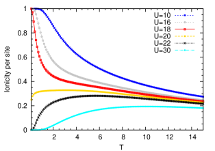
This behavior can be understood as follows: At small $U$ regime the unit cell is fully polarized at low temperatures, with both $\uparrow$ and $\downarrow$ particles occupying the A-sublattice. As the temperature is increased, some of the particles get excited to B-sublattice by absorbing the thermal energy, $k_{B}T$. Similarly for large values of $U$, at lower temperatures the unit cell is not polarized, due to the Coulomb term $U$. By increasing the temperature, thermal excitations with doubly occupied sites will be created, thereby increasing the ionicity. For intermediate $U\approx 20$, the weights of polarized and unpolarized configurations in the unit cell become comparable; hence giving the ionicity $0<I<1$.

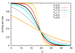
In Fig. 12 we plot the ionicity at half-filling as a function of $U$ for $\Delta=20$ and various values of $T$. As can be seen at all temperatures, the ionicity smoothly varies between $1$ for small values $U$, and $0$ for large values of $U$. The width of the transition region decreases by lowering the temperature, and is expected to approach the figure 2 of Ref. HafezCUT, .

Figure 12: Ionicity versus $U$ for some values of temperature at half-filling and $\Delta=20$.

IV Conclusion

In this work we studied a classical model consisting of two Ising like variables on a one dimensional chain. Despite the simplicity which essentially results form the lack of Fermionic minus sign problem, our model captures some of the interesting properties of the ionic Hubbard model. Various thermodynamic properties, such as, specific heat, ionicity, particle density and compressibility when viewed as a function of $U$ in a given temperature, indicate the presence of two gaped states at small and large values of $U$, with a gap-less state sandwiched between them (around $U/\Delta\approx 1$). When the same quantities viewed as a function of temperature, there is no sign of phase transition down to zero temperature. The three phase scenario of the zero temperature with clear zero temperature phase transition boundaries at $U_{c_{1}}(\Delta)$ and $U_{c_{2}}(\Delta)$ extrapolates to higher temperatures. However, the boundaries get smeared due to thermal fluctuations, giving rise to a cross-over behavior.

Mapping of $D$ dimensional quantum models to $D+1$ dimensional classical Hamiltonians is a well known paradigm in statistical physics. Our flow equation approach HafezCUT suggests an alternative approach to construct ”$D$” dimensional classical models which might be useful in capturing basic aspects of the original quantum Hamiltonian.

V Acknowledgements

We would like to thank Professor N. Nafari for useful comments and critique of the manuscript. This research was supported by the Vice Chancellor for Research Affairs of the Isfahan University of Technology (IUT). S.A.J was supported by the National Elite Foundation (NEF) of Iran.

VI Appendix

VI.1 Coefficients of Eq. (12)

The coefficients $a_{2}$, $a_{1}$, and $a_{0}$ of Eq. (12) are as follows:

$$a_{2}\equiv - \{{{\rm e}^{-\beta\,\left(2\,\widetilde{\Delta}+2\,\mu+\widetilde{U}\right)}}+2\,{{\rm e}^{-3/2\,\beta\,\left(\widetilde{\Delta}+2\,\mu\right)}}+{{\rm e}^{-\beta\,\left(4\,\mu+\widetilde{\Delta}\right)}}$$ (24)

$$+ 2\,{{\rm e}^{-1/2\,\beta\,\left(3\,\widetilde{\Delta}+2\,\mu+2\,\widetilde{U}+8\,\widetilde{V}\right)}}+4\,{{\rm e}^{-\beta\,\left(\widetilde{\Delta}+2\,\mu+2\,\widetilde{V}\right)}}$$

$$+ 2\,{{\rm e}^{-1/2\,\beta\,\left(\widetilde{\Delta}+6\,\mu\right)}}+{{\rm e}^{-\beta\,\left(2\,\widetilde{U}+8\,\widetilde{V}+\widetilde{\Delta}\right)}}+{{\rm e}^{-\beta\,\left(\widetilde{U}+2\,\mu\right)}}$$

$$+ 2\,{{\rm e}^{-1/2\,\beta\,\left(2\,\widetilde{U}+8\,\widetilde{V}+2\,\mu+\widetilde{\Delta}\right)}}\}{{\rm e}^{\beta\,\left(4\,\mu+\widetilde{\Delta}\right)}},$$

$$a_{1} \equiv -\{-4\,{{\rm e}^{-\beta\,\left(2\,\widetilde{\Delta}+2\,\mu+\widetilde{U}+2\,\widetilde{V}\right)}}+4\,{{\rm e}^{-1/2\,\beta\,\left(4\,\widetilde{U}+12\,\widetilde{V}+2\,\mu+\widetilde{\Delta}\right)}}$$ (25)

$$- 4\,{{\rm e}^{-\beta\,\left(2\,\widetilde{U}+10\,\widetilde{V}+\widetilde{\Delta}\right)}}-2\,{{\rm e}^{-1/2\,\beta\,\left(4\,\widetilde{U}+16\,\widetilde{V}+3\,\widetilde{\Delta}+2\,\mu\right)}}$$

$$- {{\rm e}^{-\beta\,\left(2\,\widetilde{U}+8\,\widetilde{V}+2\,\mu+\widetilde{\Delta}\right)}}+4\,{{\rm e}^{-1/2\,\beta\,\left(2\,\widetilde{U}+4\,\widetilde{V}+\widetilde{\Delta}+6\,\mu\right)}}$$

$$- {{\rm e}^{-\beta\,\left(2\,\widetilde{U}+\widetilde{\Delta}+2\,\mu\right)}}+4\,{{\rm e}^{-1/2\,\beta\,\left(4\,\widetilde{U}+12\,\widetilde{V}+3\,\widetilde{\Delta}+2\,\mu\right)}}$$

$$+ 4\,{{\rm e}^{-1/2\,\beta\,\left(2\,\widetilde{U}+3\,\widetilde{\Delta}+6\,\mu+4\,\widetilde{V}\right)}}-2\,{{\rm e}^{-1/2\,\beta\,\left(\widetilde{\Delta}+6\,\mu+2\,\widetilde{U}\right)}}$$

$$+ 8\,{{\rm e}^{-\beta\,\left(2\,\widetilde{\Delta}+2\,\mu+\widetilde{U}+3\,\widetilde{V}\right)}}+8\,{{\rm e}^{-\beta\,\left(4\,\mu+\widetilde{\Delta}+\widetilde{V}\right)}}-4\,{{\rm e}^{-\beta\,\left(4\,\mu+\widetilde{\Delta}\right)}}$$

$$- 4\,{{\rm e}^{-\beta\,\left(2\,\widetilde{U}+8\,\widetilde{V}+\widetilde{\Delta}\right)}}-2\,{{\rm e}^{-1/2\,\beta\,\left(4\,\widetilde{U}+3\,\widetilde{\Delta}+8\,\widetilde{V}+2\,\mu\right)}}$$

$$+ 8\,{{\rm e}^{-\beta\,\left(2\,\widetilde{U}+9\,\widetilde{V}+\widetilde{\Delta}\right)}}-2\,{{\rm e}^{-1/2\,\beta\,\left(4\,\widetilde{U}+8\,\widetilde{V}+\widetilde{\Delta}+2\,\mu\right)}}$$

$$+ 2\,{{\rm e}^{-\beta\,\left(2\,\widetilde{U}+4\,\widetilde{V}+\widetilde{\Delta}+2\,\mu\right)}}-4\,{{\rm e}^{-\beta\,\left(2\,\widetilde{\Delta}+2\,\mu+\widetilde{U}+4\,\widetilde{V}\right)}}$$

$$- 4\,{{\rm e}^{-\beta\,\left(\widetilde{U}+2\,\widetilde{V}+2\,\mu\right)}}-2\,{{\rm e}^{-1/2\,\beta\,\left(2\,\widetilde{U}+3\,\widetilde{\Delta}+6\,\mu+8\,\widetilde{V}\right)}}$$

$$- 2\,{{\rm e}^{-1/2\,\beta\,\left(4\,\widetilde{U}+16\,\widetilde{V}+2\,\mu+\widetilde{\Delta}\right)}}-2\,{{\rm e}^{-1/2\,\beta\,\left(2\,\widetilde{U}+6\,\mu+8\,\widetilde{V}+\widetilde{\Delta}\right)}}$$

$$- 2\,{{\rm e}^{-1/2\,\beta\,\left(2\,\widetilde{U}+3\,\widetilde{\Delta}+6\,\mu\right)}}-4\,{{\rm e}^{-\beta\,\left(4\,\mu+\widetilde{\Delta}+2\,\widetilde{V}\right)}}$$

$$+ 8\,{{\rm e}^{-\beta\,\left(\widetilde{U}+3\,\widetilde{V}+2\,\mu\right)}}-4\,{{\rm e}^{-\beta\,\left(\widetilde{U}+4\,\widetilde{V}+2\,\mu\right)}}\}{{\rm e}^{\beta\,\left(\widetilde{\Delta}+6\,\mu\right)}},$$

$$a_{0} \equiv 4\,{{\rm e}^{-2\,\beta\,\left(\widetilde{U}+\widetilde{V}-3\,\mu\right)}}\{-4\,{{\rm e}^{-2\,\beta\,\widetilde{V}}}-4\,{{\rm e}^{-5\,\beta\,\widetilde{V}}}-4\,{{\rm e}^{-3\,\beta\,\widetilde{V}}}$$ (26)

$$+ 10\,{{\rm e}^{-4\,\beta\,\widetilde{V}}}+4\,{{\rm e}^{-\beta\,\widetilde{V}}}+4\,{{\rm e}^{-7\,\beta\,\widetilde{V}}}-4\,{{\rm e}^{-6\,\beta\,\widetilde{V}}}$$

$$- {{\rm e}^{-8\,\beta\,\widetilde{V}}}-1\}.$$

References

- (1) G.F. Newell and E.W. Montroll, Rev. Mod. Phys. 25, (1953) 353.
- (2) R.P. Feynman, Statistical Mechanics, Westview Press, 1998.
- (3) E. Fradkin, Field Theories of Condensed Matter Systems, Westview Press, 1998.
- (4) L. Onsager, Phys. Rev. 65, (1944) 117.
- (5) S. A. Jafari Int. J. Mod. Phys. B 23, (2009) 395.
- (6) N. Nagaosa, J. Takimoto, J. Phys. Soc. Jpn. 55 (1986) 2735.
- (7) T. Egami S. Ishihara, M. Tachiki Science 261 (1993) 1307.
- (8) M. Hafez, S. A. Jafari M. R. Abolhassani Phys. Lett. A, 373 (2009) 4479.
- (9) M. Fabrizio, A. O. Gogolin and A. A. Nersesyan, Phys. Rev. Lett. 83 (1999) 2014; C. D. Batista and A. A. Aligia, Phys. Rev. Lett. 92 (2004) 246405; S. R. Manmana, V. Meden, R. M. Noack, and K. Schönhammer, Phys. Rev. B 70 (2004) 155115; Ö. Legeza, K. Buchta, and J. Sólyom, Phys. Rev. B 73 (2006) 165124; T. Wilkens and R.M. Martin, Phys. Rev. B 63 (2001) 235108; S. S. Kancharla and E. Dagotto, Phys. Rev. Lett. 98 (2007) 016402.
- (10) K. Bouadim, N. Paris, F. Hébert, G. G. Batrouni and R.T. Scalettar, Phys. Rev. B 76 (2007) 085112;
- (11) A. Garg, H. R. Krishnamurthy, and M. Randeria, phys. Rev. Lett. 97 (2006) 046403; N. Gidopoulos, S. Sorella, E. Tosatti E. Phys. J. B 14 (2000) 217; N. Paris, K. Bouadim, F. Hébert, G. G. Batrouni and R. T. Scalettar, Phys. Rev. Lett. 98 (2007) 046403;
- (12) S. A. Jafari et al., unpublished.
- (13) N. Goldenfeld, Lecture on Phase Transitions and The Renormalization Group, Westview Press, 1992.