REM near-IR and optical photometric monitoring of Pre-Main Sequence Stars in Orion. ^{, ,}

Abstract

Aims. We aim at determining the rotational periods and the starspot properties in very young low-mass stars belonging to the Ori OB1c star forming region, contributing to the study of the angular momentum and magnetic activity evolution in these objects.

Methods. We performed an intensive photometric monitoring of the PMS stars falling in a field of about 10$\arcmin\times 10\arcmin$ in the vicinity of the Orion Nebula Cluster (ONC), also containing the BD eclipsing system 2MASS J05352184-0546085. Photometric data were collected between November 2006 and January 2007 with the REM telescope in the $VRIJHK^{\prime}$ bands. The largest number of observations is in the $I$ band (about 2700 images) and in $J$ and $H$ bands (about 500 images in each filter). From the observed rotational modulation, induced by the presence of surface inhomogeneities, we derived the rotation periods. The long time-baseline (nearly three months) allowed us to detect rotation periods, also for the slowest rotators, with sufficient accuracy ($\Delta P/P<2\%$). The analysis of the spectral energy distributions and, for some stars, of high-resolution spectra provided us with the main stellar parameters (mass, luminosity, effective temperature, mass, age, and $v\sin i$) which are essential for the discussion of our results. Moreover, the simultaneous observations in six bands, spanning from optical to near-infrared wavelengths, enabled us to derive the starspot properties for these very young low-mass stars.

Results. In total, we were able to determine the rotation periods for 29 stars, spanning from about 0.6 to 20 days. Thanks to the relatively long time-baseline of our photometry, we derived periods for 16 stars and improved previous determinations for the other 13. We also report the serendipitous detection of two strong flares in two of these objects. In most cases, the light-curve amplitudes decrease progressively from the $R$ to $H$ band as expected for cool starspots, while in a few cases, they can only be modelled by the presence of hot spots, presumably ascribable to magnetospheric accretion. The application of our own spot model to the simultaneous light curves in different bands allowed us to deduce the spot parameters and particularly to disentangle the spot temperature and size effects on the observed light curves.

1 Introduction

The study of the evolution of angular momentum of low-mass stars in the pre-main sequence (PMS) phase has gained great advantage from high-precision photometry of star forming regions (SFR). While during the main sequence (MS) evolutionary phase the total angular momentum of a solar-mass star is lost efficiently via the magnetic-wind breaking process (e.g., Chaboyer et al. 1995), in the PMS phase the presence of a circumstellar disc coupled to the star through magnetic fields permits a more efficient angular momentum transfer, thus preventing the spin-up driven by the rapid mass-accretion and contraction of the star (Shu et al. 1994).

An accurate knowledge of the rotation period distribution of the solar and low-mass stars in different SFR environments is of paramount importance for understanding how the disc-locking mechanism is effective in modifying the angular momentum in the PMS stage, and for testing the reliability of the theoretical models of PMS star interiors and their evolutionary tracks.

Measurements of periodic light-variations with typical amplitudes in the range 0.05–0.40 mag in the $V$ and $R$ bands, due to uneven starspot distributions on the stellar photospheres, are a direct way to obtain this physical parameter. There has been a rapid increase in the number of PMS objects with measured rotation periods over the last decade (see, e.g., Mathieu 2004; Herbst et al. 2007; Irwin & Bouvier 2009, and references therein). A broad, bimodal distribution exists at the earliest observable phases (about 1 Myr) for stars more massive than 0.4 M_☉. The fast rotators (50–60% of the sample) evolve to the ZAMS with little or no angular momentum loss. The slow rotators continue to lose substantial amounts of angular momentum for up to 5 Myr, creating the even broader bimodal distribution characteristic of 30–120 Myr old clusters. Accretion disc signatures, such as H$\alpha$ emission and infrared (IR) excess, are observed more frequently among slowly rotating PMS stars, suggesting a connection between accretion and rotation (Rebull et al. 2006). According to the present picture, discs appear to influence rotation only for a small percentage of the solar-type stars and only during the first 5 Myr of their life. This time interval is comparable to the maximum life-time of accretion discs derived from NIR studies and may be a useful upper limit to the time available for forming giant planets. For the sparse population of young stars (mainly weak-T Tauri stars, wTTS, with ages between 5 and 30 Myr) in the Orion complex, Marilli et al. (2007) found no evidence of bimodality for masses higher than 0.7 M_☉, and a median rotation period of $\sim$ 1.5 days, suggesting that the spin-up process at this stage has become dominant over the disc-locking effect. It is then mandatory to explore the rotational properties of as many clusters/associations as possible with ages less than 5 Myr. Indeed, in this age range, the different scenarios for angular momentum evolution proposed by Lamm et al. (2005) and related to different time-scales of disc-locking and stellar contraction (Hartmann 2002) are expected to produce their stronger effects.

There is growing evidence that the same mechanisms operating in solar-mass stars also regulate the rotation of very-low mass (VLM) stars and brown dwarfs (BDs). Indeed, very recently many BDs showing accretion discs with physical properties similar to their analogs around higher-mass stars have been discovered (e.g., Luhman et al. 2005; Alcalá et al. 2006; Muzerolle et al. 2006; Merín et al. 2007, and reference therein). However, it seems that both disc interactions and stellar winds are less efficient in braking these objects, although the statistics available for this VLM regime is rather poor.

In some cases, both VLM and BD objects in star forming regions exhibit photometric light curves with high amplitudes and irregular modulations (Scholz & Eislöffel 2004, 2005) that are usually explained by hot spots caused by mass-accretion flow from the disc (Herbst 1994). The same authors remark that wTTS and some classical T Tau stars (cTTS) display instead more regular light curves with smaller amplitudes ascribable to cool photospheric spots that can survive for several stellar rotations.

In this paper, we report the results of an intensive photometric monitoring, in near-infrared (NIR) and optical bands, of a sample of young low-mass stellar and sub-stellar objects (YSOs) in a small area flanking the Orion Nebula Cluster (ONC). The main goal of our observations was the study of the NIR light curve of 2MASS J05352184-0546085, an eclipsing system composed of two BD components recently discovered by Stassun et al. (2006). The long-lasting and intensive simultaneous optical and NIR monitoring also allowed us to study the photometric variability of many YSOs in the field of view around the eclipsing BD. Therefore, in this study we report the characterization of these objects and determine their rotational periods, as well as the properties of their starspots. The present work thus contributes to the study of the early phases of angular momentum evolution and of the behaviour of magnetic activity in young, VLM objects which still needs observational and interpretation efforts.

We derived the rotation periods of our targets by means of time-series analysis of our large photometric data-set gathered in the $VRIJHK^{\prime}$ bands. The physical characterization (radius, luminosity, effective temperature, mass, and age) of the objects, which is essential for any discussion on angular momentum evolution and stellar activity, is based on our photometric data as well as on literature mid-IR data from the Spitzer space telescope (Rebull et al. 2006) through an analysis of their spectral energy distribution (SED). For some objects, accurate physical parameters and the projected rotational velocity, $v\sin i$, were determined by means of high-resolution spectra.

The use of simultaneous multi-band light curves allows an accurate analysis of the spot properties because the different amplitude of the light curves constrains the spot temperatures and filling factors.

2 Observations and data reduction

The observations were performed with REM (Rapid Eye Mount), a 60-cm robotic telescope located at the ESO-La Silla Observatory (Chile), on 66 nights from November 2nd, 2006 to January 20th, 2007. By means of a dichroic, REM feeds simultaneously two cameras at the two Nasmyth focal stations, one for the NIR (REMIR) and one for the optical (ROSS). The cameras have nearly the same field of view of about 10$\arcmin\times 10\arcmin$ and use wide-band filters ($z^{\prime}$, $J$, $H$, and $K^{\prime}$ for REMIR and $V$, $R$, and $I$ for ROSS). The main scientific aim of REM is the study of the early phases of after-glow of gamma-ray bursts detected by space-borne high-energy alert systems. Even if the schedule of REM is optimized to collect as many triggers as possible from active space-borne observatories, a considerable amount of time can be spent on additional science.

We selected a 10$\arcmin$ field flanking the ONC that included the eclipsing BD binary 2MASS J05352184-0546085 (Stassun et al. 2006). To this purpose, we observed mainly in the $I$-band with ROSS and in $JHK^{\prime}$ with REMIR. In total, we collected 184, 175, 2769, 514, 461, and 250 usable images in $V$, $R$, $I$, $J$, $H$, and $K^{\prime}$ bands, respectively. Exposure times were typically of 60–120 seconds in the optical bands and of 30–60 seconds in $JHK^{\prime}$. Longer exposure times were not adopted in order to avoid image blurring by the guiding/de-rotating system.

Full phase coverage of the primary eclipse was not achieved during the observing season due to bad weather and technical problems. Also, the telescope size and relatively short exposure times were not sufficient to obtain high quality light curves of 2MASS J05352184-0546085 worthy of being analyzed (see Fig. 1). During the final redaction of the present manuscript, we saw the very recent paper of Gómez Maqueo Chew et al. (2009) where complete and more accurate $JHK$ light curves of 2MASS J05352184-0546085, are presented and analyzed.

Figure 1: REM light curves of the eclipsing binary 2MASS J05352184-0546085 composed of two BDs, in the $I$, $J$, and $H$ bands. Photometric points are phased according to the ephemeris of Stassun et al. (2006). The average error bar for each band is also shown. The phases of the primary and secondary minimum are marked, in the lower box, by vertical continuous and dashed lines, respectively.

However, the long-lasting and intensive simultaneous optical and NIR monitoring allowed us to detect and study the photometric variability of several objects in this 10$\arcmin$ field of view. In particular, we measured the magnitudes for 97 stars brighter than, or comparable to, 2MASS J05352184-0546085 in $JHK^{\prime}$. For 58 of these stars, we were also able to measure $RI$ (and for 47 of them also $V$) magnitudes. Some stars were too faint to be detected in the optical bands, or situated near the edges of the REMIR field of view and outside of the optical frames. Therefore, due to slight random shifts in the field centering from one pointing to another, the closer to the border, the poorer was the data sampling for these stars. Very close pairs (separation $\leq 7\arcsec$) are not considered in the following analysis.

The field of view, as observed in the $H$ filter, together with the identification code given by us to the above mentioned stars, is displayed in Fig. 2.

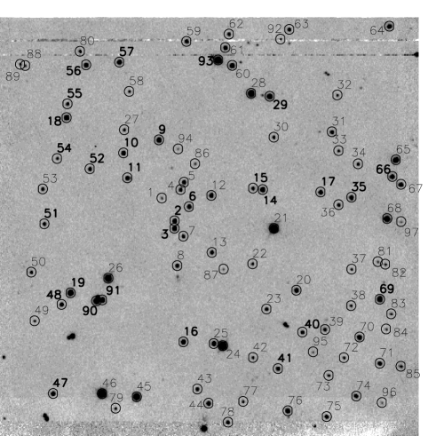
Figure 2: Finding chart of the objects investigated in the present paper. The identification code (Id in Table 2) is written in boldface for the stars which display periodic variations. The image is taken with the REMIR camera in the $H$ band. The central coordinates at J2000 are RA=$05^{\rm h}35^{\rm m}16\aas@@fstack{s}7$, DEC=$-05\degr 46\arcmin 43\arcsec$. Orientation: North is up, East to the left.

The pre-reduction of the REMIR images is automatically done by the AQuA pipeline (Testa et al. 2004) and the co-added and sky-subtracted frames, resulting from five individual ditherings, are made available to the observer.

For the ROSS camera, the data reduction was more complex. Indeed, the field of view is vignetted and the non-uniform illumination of the CCD changes with the de-rotator position. Since twilight flat-fields were not available, we built up master-flats at the four different de-rotator orientations by using scientific images of our field and several standard-star fields separately for the $V$, $R$, and $I$ filters. Each scientific image, after subtraction of the dark-frame, was divided by the proper master-flat, depending on the filter and de-rotator orientation. We verified that the scatter in the data is strongly reduced this way.

2.1 Differential photometry

Aperture photometry for all the selected stars was performed with DAOPHOT by using the IDL routine Aper. The photometric errors due to the photon statistics in the NIR bands are of about 0.04–0.06 mag for the faintest stars ($H\,\simeq 14$ mag), while they are as low as 0.001 mag for the brightest stars ($H\,\simeq 9$ mag) in the field. In the $I$ band, a faint star ($I\,\simeq 17$ mag) has a photometric error of about 0.10 mag, while for a bright one ($I\,\simeq 12$ mag) the photon statistics gives rise to a 0.001-mag error.

We calculated the differential magnitude of each target with respect to an artificial comparison star built-up using all the non-variable stars present in the field. We used the approach of Broeg et al. (2005), which consists in comparing each star with an artificial comparison composed by all the other stars in the field. An iterative process allowed us to identify the variable objects and separate them from those that are best suited to construct the artificial comparison, by weighting them down according to their variability. This method has also the advantage of providing reliable error bars. The final errors derived with this algorithm turn out to be of about 0.10 mag for a star with $I\,\simeq 17$ mag, while for the brightest stars in $I$-band we obtain an error of $\simeq 0.02$ mag. In the NIR bands, we have a typical error of $\sim 0.09$ mag for a star with $H=14$ mag, while an error of about 0.02 mag is found for the brightest stars. The photometric accuracy achieved is mainly limited by the quality of the flat-field correction, due to the complexity of the instrument.

2.2 Standard photometry

In order to transform the $V,R$ and $I$ instrumental magnitudes to the standard Johnson-Cousins system, some stars in the Landolt standard fields SA 98, SA 94, and SA 96 (Landolt 1992), observed by REM during the season of our observations, were used. The standard $V$, $R$, and $I$ magnitudes were determined using the transformation equations:

$$V=v-\kappa_{V}\cdot AM+c_{V}\cdot(V-R)+ZP_{V}$$ (1)

$$R=r-\kappa_{R}\cdot AM+c_{R}\cdot(R-I)+ZP_{R}$$ (2)

$$I=i-\kappa_{I}\cdot AM+c_{I}\cdot(R-I)+ZP_{I}$$ (3)

where $v$, $r$, and $i$ are the instrumental magnitudes, $\kappa$ the coefficients of atmospheric extinction, $AM$ the airmass, and $c_{V}$ and $ZP_{V}$, $c_{R}$ and $ZP_{R}$, and $c_{I}$ and $ZP_{I}$ the color terms and zero-points for the $V$, $R$, and $I$ bands, respectively.

We determined the atmospheric extinction coefficients using the non-variable stars in our Orion field observed, during some nights, across a suitable airmass range. Their values, listed in Table 1, are however not very different from the mean extinction coefficients for La Silla.

The standard magnitudes from Stetson (2000) were used to determine the zero-points and color terms for the SA 98 area (Table 1). Forty-five sufficiently bright stars with standard magnitudes in the Stetson (2000) catalogue fall within the REM $10\arcmin\times 10\arcmin$ field centered around the star SA 98-978. Unfortunately, this standard field was observed six hours later than the Orion field on December 23, 2006. The zero-points determined on January 17th and 18th, 2007 by means of the stars SA~94-242 and SA~96-36 are also listed in Table 1. We adopted these zero-points for the standardization of the magnitudes on January 17 and 18, 2007. Indeed, these standard stars were observed within 30 minutes from the Orion field. The standard magnitudes evaluated in these two dates allowed us to transform the differential light curves into standard ones.

Table 1: Atmospheric extinction and photometric calibration coefficients.

Filter	$\kappa$	$c^{\rm a}$	$ZP^{\rm a}$	$ZP^{\rm b}$	$ZP^{\rm c}$
$V$	0.187	$-0.108$	20.899$\pm$0.024	20.874	20.954
$R$	0.135	$-0.110$	21.208$\pm$0.030	21.202	21.220
$I$	0.072	$-0.147$	20.629$\pm$0.020	20.577	20.608

• From SA 98 standard area observed on December 23, 2006.

• From SA 94-242 observed on January 17, 2007.

• From SA 96-36 observed on January 18, 2007.

The conversion of the instrumental magnitudes $j$, $h$, and $k^{\prime}$ to the standard $JHK^{\prime}$ was performed by defining, for each frame, a zero-point by means of all the non-variable stars in the Orion field, whose magnitudes were taken from the 2MASS catalogue (Cutri et al. 2003). Since these stars were observed simultaneously with the variable ones, no correction for the airmass was needed.

The standard $VRIJHK^{\prime}$ average magnitudes derived by us are listed in Table LABEL:tab:VRIJHK together with the IRAC Spitzer magnitudes in mid-IR bands (3.6, 4.5, 5.8, 8 $\mu$m) reported for a few of them by Rebull et al. (2006).

A very interesting outcome of the intensive monitoring in the $I$ band was the detection of a strong flare of the star #19 (2MASS~J05352973-0548450 = V498~Ori) occurred on December 7th 2006, reaching the peak intensity ($\Delta I\approx 0.3$ mag) at about 04:41 UT, with a total duration of nearly 2 hours (Fig. 3). Unfortunately, we lack simultaneous $V$ and $R$ data. Notwithstanding the smaller time resolution, a small flux intensification ($\Delta J\approx 0.1$ mag) seems to be present in the $J$-band as well, while no clear enhancement emerges in the $H$-band. The data points corresponding to this flare event were excluded from the following time-series analysis. Another strong flare ($\Delta I\approx 0.8$ mag) was observed on star #11 (2MASS~J05352550-0545448 = NR~Ori) on December 10th 2006 at $\approx$ 01:30 UT and lasted for about 2 hours (Fig. 21). In this case, no significant enhancement emerges in the simultaneous $J$ light curve.

Figure 3: The flare event observed on Star #19 (2MASS J05352973-0548450) on December 7th, 2006 at 4:41 UT in the $I$ band (upper panel). The simultaneous $J$ and $H$ light curves are also displayed in the two bottom panels.

2.3 Complementary spectroscopic data

Spectroscopic observations of some of the stars observed with REM were carried out using the Hectochelle multi-object spectrograph (Szentgyorgyi 1998) at the 6.5-m MMT telescope in Arizona. These data were used by Fűrész et al. (2008) and Tobin et al. (2009) to study the kinematics of the Orion nebula clusters.

The resolution was $R\simeq 34\,000$ and the spectra observed in 2004 and 2005 (Fűrész et al. 2008) are centered at H$\alpha$ and span 190 Å, while those acquired in 2006 and 2007 (Tobin et al. 2009) cover the spectral range $\lambda$5150–5300 Å, which includes the Mg i b triplet. The reader is referred to the aforementioned papers for further details about observations and data reduction.

3 Time-series analysis and rotation periods

We derived the periods of the light variations by applying to the best light curves (typically $R$, $I$, $J$, and $H$ bands) a periodogram analysis (Scargle 1982) and the CLEAN deconvolution algorithm (Roberts et al. 1987), which allowed us to reject aliases generated by the spectral window of the data. We also evaluated the period uncertainty following the prescriptions of Horne & Baliunas (1986). The frequency uncertainty can be written as

$$\Delta\nu=\frac{3\sigma_{\rm N}}{4\sqrt{N_{0}}\,T\,A},$$ (4)

where $\sigma_{\rm N}^{2}$ is the data variance, $T$ the total time-span of the data, $A$ the amplitude of the signal, and $N_{0}$ the number of independent points. We considered two data points independent (uncorrelated) if those were spaced in time by more than 0.05 in period units. Another estimate of the frequency uncertainty is provided by the full width at half maximum (FWHM) of the periodogram peak. In this case, the values are typically 10–20 times larger than those calculated through Eq. 4 and reported in Table 2. However, even adopting uncertainties based on the FWHM of the peak, our results do not change.

The period of variation was taken as the reciprocal of the frequency of the highest peak in the cleaned power spectrum. Usually, the most accurate periods were found for the $I$ light curves, mainly because of the very large number of data-points and relatively large amplitudes. For some of the reddest objects we found instead better period determinations (smaller errors) in the $J$ or $H$ filters. The variation periods are listed in Table 2 together with the bands in which they have been detected (ordered according to increasing period errors). The light-curve amplitudes in the $VRIJHK^{\prime}$ bands and previous period determinations from the literature (Stassun et al. 1999; Carpenter et al. 2001; Rebull 2001; Rebull et al. 2006) are also reported in this table.

Table 2: Rotation periods ($P$), false-alarm probabilities (FAP), and light-curve amplitudes ($\Delta V$, $\Delta R$, $\Delta I$, $\Delta J$, $\Delta H$, and $\Delta K^{\prime}$) of our targets. A colon marks periods with FAP$>$ 5%.

Id	$P$	Err	FAP	Band	$\Delta V$	$\Delta R$	$\Delta I$	$\Delta J$	$\Delta H$	$\Delta K^{\prime}$	$P_{\rm Stas}^{\mathrm{a}}$	$P_{\rm Reb}^{\mathrm{b}}$	$P_{\rm Carp}^{\mathrm{c}}$
	(days)	(days)			(mag)	(mag)	(mag)	(mag)	(mag)	(mag)	(days)	(days)	(days)
1	9.78c	…	…	…	…	…	…	…	…	…	9.78d	…	…
2	7.751	0.108	3$\cdot 10^{-5}$	$RIJH$	…	0.085	0.065	0.040	0.035	0.025	…	…	…
3	1.311	0.003	1$\cdot 10^{-10}$	$IHJ$	0.050	…	0.040	0.030	0.030	0.020	…	…	…
5	…	…	…	…	…	…	…	…	…	…	…	0.60	…
6	5.993	0.070	6$\cdot 10^{-3}$	$IRJH$	0.090	0.065	0.040	0.020	0.020	0.020	…	…	…
9	0.5627	0.0002	1$\cdot 10^{-11}$	$IJHR$	0.090	0.100	0.065	0.040	0.040	0.045	0.57	…	…
10	5.816	0.010	1$\cdot 10^{-6}$	$RIHJ$	0.365	0.345	0.280	0.140	0.150	0.125	…	5.90	5.88
11	7.383	0.003	1$\cdot 10^{-6}$	$HJIR$	0.850	0.970	1.150	1.250	1.180	0.900	…	7.50	7.46
14	4.047	0.003	5$\cdot 10^{-10}$	$IHJR$	0.390	0.345	0.265	0.135	0.145	0.125	4.02	4.04	3.98
15	11.86:	0.08	9$\cdot 10^{-2}$	$IJH$	…	…	0.160	0.030	0.035	0.030	…	…	…
16	6.351	0.072	2$\cdot 10^{-2}$	$IRJH$	0.145	0.130	0.055	0.035	0.035	0.030	…	…	…
17	8.435	0.020	1$\cdot 10^{-4}$	$IHJR$	0.395	0.290	0.245	0.125	0.130	0.115	7.70	4.18	…
18	12.461	0.069	1$\cdot 10^{-7}$	$RIHJ$	0.285	0.225	0.110	0.055	0.055	0.035	…	…	…
19	0.605	0.035	4$\cdot 10^{-4}$	$JI$	…	…	0.060	0.030	…	…	…	…	…
29	8.468	0.046	1$\cdot 10^{-2}$	$IJR$	0.175	0.150	0.145	0.040	0.050	…	…	…	…
35	12.521	0.218	3$\cdot 10^{-4}$	$HJ$	…	…	…	0.070	0.070	…	…	12.41	…
40	5.297	0.007	5$\cdot 10^{-7}$	$HJ$	…	…	…	0.275	0.270	0.250	…	…	…
41	6.783	0.040	2$\cdot 10^{-2}$	$JHIR$	0.260:	0.205	0.125	0.075	0.090	0.110	…	…	…
47	10.02	0.21	5$\cdot 10^{-2}$	$HJ$	…	…	…	0.055	0.055	…	9.60	10.08	…
48	7.721	0.019	2$\cdot 10^{-4}$	$IHJ$	…	…	0.280	0.270	0.230	…	…	…	…
51	2.763	0.010	2$\cdot 10^{-2}$	$IJH$	…	…	0.040	0.025	0.025	0.025	…	2.81	…
52	1.696	0.004	1$\cdot 10^{-2}$	$IJHR$	0.170	0.090	0.070	0.030	0.035	0.050	1.69	1.70	…
54	2.514	0.002	5$\cdot 10^{-12}$	$JHI$	…	…	0.315	0.265	0.235	0.190	…	…	…
55	8.432	0.035	5$\cdot 10^{-6}$	$IRJH$	0.300:	0.230	0.135	0.070	0.120	…	8.06	…	…
56	3.80	0.06	3$\cdot 10^{-2}$	$R$	…	0.065	…	…	…	…	3.86	3.84	…
57	4.647	0.038	1$\cdot 10^{-2}$	$JIR$	0.185	0.120	0.050	0.040	…	…	…	…	…
59	…	…	…	…	…	0.5	0.4	0.3	…	…	7.33	7.33	…
60	…	…	…	…	…	…	…	…	…	…	4.04	4.11	4.09
61	…	…	…	…	…	1.5	0.8	0.6	…	…	…	18.68	…
62	…	…	…	…	…	…	…	…	…	…	2.05	2.05	…
63	…	…	…	…	…	…	…	…	…	…	1.10	1.09	…
66	21.68:	0.30	1$\cdot 10^{-1}$	$HJ$	…	…	…	0.40	0.40	…	…	59.87	14.62
69	6.550	0.068	5$\cdot 10^{-3}$	$JH$	…	…	…	0.060	0.050	…	…	…	…
75	…	…	…	…	…	…	…	…	…	…	…	10.71	…
90	4.376	0.013	1$\cdot 10^{-5}$	$IJRH$	0.205	0.135	0.120	0.055	0.040	…	…	…	…
91	10.176	0.055	2$\cdot 10^{-5}$	$JHIR$	…	0.070	0.080	0.090	0.095	0.070	…	…	…
93	5.70:	0.12	2$\cdot 10^{-1}$	$IJ$	…	…	0.150	0.200	…	…	…	5.53	5.53

• Rotational periods derived by Stassun et al. (1999).

• Rotational periods derived by Rebull (2001) or Rebull et al. (2006).

• Rotational periods derived by Carpenter et al. (2001).

• Orbital period from Stassun et al. (2006), and confirmed by us.

In total, we determined the rotation periods for 29 stars. Thirteen of these had periods previously detected, while for all the others the period is derived here for the first time. In fact, observations in different observing seasons may be necessary to detect as many rotation periods as possible, as shown, e.g., by Parihar Padmakar et al. (2009) for some ONC stars. Indeed, depending on the spottedness level and the spot distribution over the photosphere, the amplitude of the light variation may sometimes be too small for detecting a periodic modulation.

On the other hand, we could not detect any reasonable periodicity in our data of 7 stars (also included in Table 2) for which the aforementioned authors did. However, we note that, except for star #5, all of them lie near the edges or out of the field, and/or close to bad columns of the ROSS and REMIR detectors (cf. Fig. 2) and, consequently, we have for them a lower number of useful data points. Two of them (#59 and #61) display large non-periodic variations, as discussed later in this section, while, for the remaining five, no significant variation has been detected.

False-alarm probabilities (FAP) for the peaks in the periodograms were also computed according to the definitions given by Scargle (1982) and by Horne & Baliunas (1986). As stressed by Horne & Baliunas (1986), the FAP depends on the data sampling and can be lowered by a large number of data points taken so close in time that they do not really represent independent measurements and tend to inflate the power artificially. Therefore, we adopted the number of independent points $N_{0}$, evaluated as described above, for the FAP computation.

With the exception of only three stars (i.e., #15, #66 and #93), the periods are detected with a FAP$\leq$ 5%, i.e. with a high confidence level (1-FAP$\geq$ 95%). The periods of the three stars with a high FAP are considered only as possible detections and are marked with a colon in Table 2. In order to check the reliability of these FAPs, we run 1000 Monte Carlo simulations of photometric sequences with only noise and with the same time sampling of $I$ data and measured the power of the highest peak in the periodogram of each sequence. Comparing periodogram peak heights of the real data with the cumulative distribution of the peak heights in the simulated data, we found that all stars with very low FAPs in Table 2 have indeed a FAP$<$0.001.

The LC collection is displayed in Fig. 4, where the source identifiers and the photometric periods are indicated.

A very peculiar light curve, which shows two diagonal strips resembling eclipse egresses around phase 0.2 and 0.4, is displayed by star #48 (2MASS J05353047-0549037). At the beginning we thought that this star could be an eclipsing binary. However, we could not find any period suitable to fold these steep variations into a phased eclipsing binary light curve. We have no clear explanation for such a behaviour and we can only speculate that these features might be produced by distinct objects/dust-clumps (protoplanetary condensations?) transiting over the apparent stellar disc. More repeated observations are needed to settle this point.

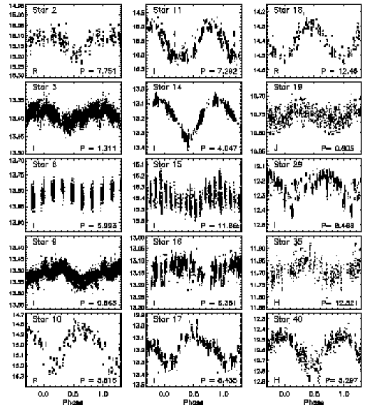
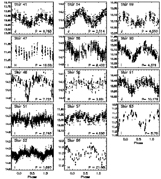
Figure 4: Phase-folded light curves of the objects with detected period in the 2MASS J05352184-0546085 field. Source Id and observed band are also indicated in each box.

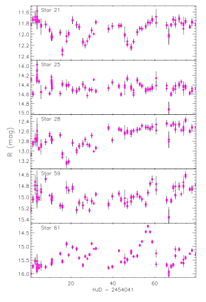
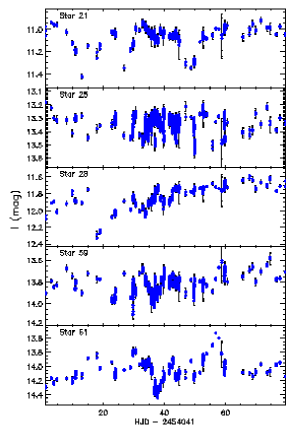
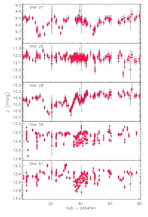
Figure 22: Light curves in the $R$, $I$, and $J$ band of the five variable stars for which we could not find any reliable period.

In order to pick up all the variable stars in our field, we applied a $\chi^{2}$ test on the $I$-band photometric sequences. We found only five bona-fide variables (with a reduced chi-square $\chi_{\nu}^{2}>3$) showing non-periodic variations as large as 0.6 magnitudes (#21, #25, #28, #59, and #61). Their $R$, $I$, and $J$ light curves are displayed as a function of the heliocentric Julian day in Fig. 22. We note that, with the exception of star #25, all the others were already classified as variable stars.

4 Spectral Energy Distributions and stellar parameters

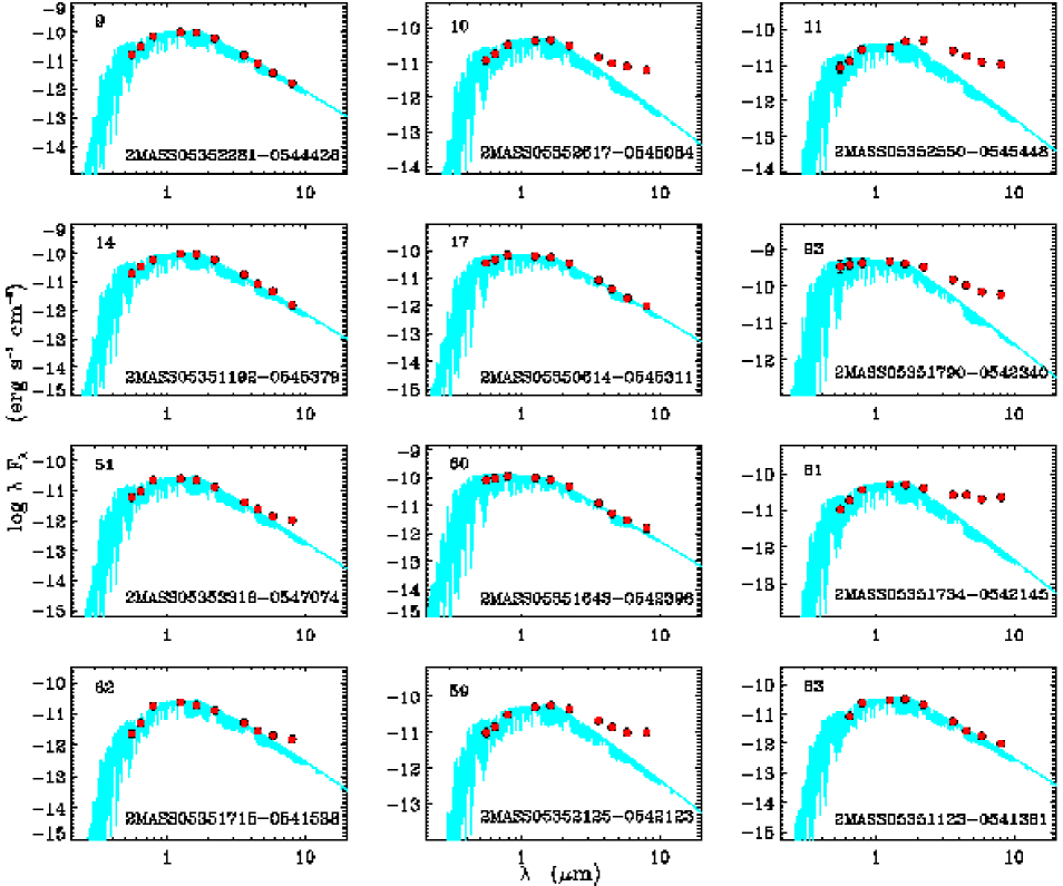
Figure 5: Spectral energy distributions for the 12 stars with available IRAC mid-IR fluxes (dots). The best-fit NextGen spectrum is over-plotted with continuous lines in each box. The entry number in Table 2 and the 2MASS identifier are also indicated in each box.

The standard $VRIJHK^{\prime}$ photometry (Table LABEL:tab:VRIJHK) allowed us to derive the spectral energy distribution (SED), from the optical to NIR, for a sub-sample of 66 sources. For 58 of these we used our own ROSS and REMIR photometry, while for 8 objects we appended $V$ and/or $I$ magnitudes retrieved from the literature (Rebull et al. 2000; Rebull 2001; DENIS 2005; Lasker et al. 2008) to our own $JHK^{\prime}$ data. For 14 objects we made also use of the Spitzer IRAC magnitudes from Rebull et al. (2006), extending the SED to the mid-IR. We then adopted the grid of NextGen low-resolution synthetic spectra, with $\log g=3.5$ and solar metallicity by Hauschildt et al. (1999), to perform a three-parameter fit to the SEDs. The stellar radius ($R_{*}$), effective temperature ($T_{\rm eff}$), and interstellar extinction ($A_{V}$) are free parameters of the fit. The Cardelli et al. (1989) extinction law with $R_{V}=3.1$ was used. To convert the apparent magnitudes into absolute ones, we assumed the ONC distance $d=414\pm 7$ pc (Menten et al. 2007). The best solution was found by minimizing the $\chi^{2}$ of the fit, which was performed only when $VRIJHK^{\prime}$ data were available. Figure 5 displays the results of the fitting procedure for 12 of the stars with IRAC mid-IR flux measurements available. The stellar luminosity was then obtained by integrating the best-fit model spectrum.

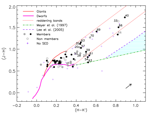
Figure 6: NIR color-color diagram for the sources in our sample. The continuous lines represent the colors for dwarfs and giants as labelled. The reddening direction is indicated by the dotted lines. The $A_{\rm V}=1$ mag reddening vector is also shown. The locus of strong NIR excess (hatched area) is defined by the criteria of Meyer et al. (1997) and Lee et al. (2005) as labelled. Members and non-members are represented by filled and open circles, respectively. Black-filled circles indicate objects with a period determination. Crosses represent sources with only $JHK^{\prime}$ data.

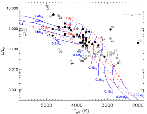
Figure 7: HR diagram of the objects with standard photometry listed in Table LABEL:tab:VRIJHK. Star symbols have been used for the objects with $T_{\rm eff}$ derived from spectra, while the other objects are represented with circles. Black symbols refer to stars with period determination. Objects falling in a position not consistent with the Orion cloud (open symbols) are also labelled with their Id number. The two asterisks mark the positions of the individual components of the BD eclipsing binary according to Stassun et al. (2006). The evolutionary PMS tracks and isochrones by Baraffe et al. (1998) and Chabrier et al. (2000) are also displayed in the figure by continuous and dotted lines, respectively.

For the 15 stars with Hectochelle spectra and for star #93 (Wolff et al. 2004), we performed the SED fit by fixing the effective temperature to the value derived from the corresponding high-resolution spectrum (see Sect. 5). These values are reported in Table 4, while in Table 3 the Id and $T_{\rm eff}$ values for these stars are listed in italic characters. By comparing these values with those coming from the SED fits, i.e. assuming $T_{\rm eff}$ as a free parameter, they result to be in agreement within 200 K, which is the typical uncertainty on $T_{\rm eff}$ when derived from SED fits (Gandolfi et al. 2008). However, the fits may underestimate $T_{\rm eff}$ by several hundred degrees in the case of high extinction and/or strong NIR excess. To investigate this, we use the NIR color-color diagram shown in Fig. 6, where the stars with the parameters derived from the SED analysis are represented by circles, while those ones with only $JHK^{\prime}$ photometry are indicated by crosses. Although none of the sources fall in the region typical of very strong NIR excess, most objects appear moderately reddened ($A_{V}<$ 1 mag); however, 17 objects among those with SED available (labelled with their Id in Fig. 6) have probably a higher extinction. In particular, two of the brightest variable stars (#21 and #28) as well as star #70 seem to have a higher reddening. In fact, the SED analysis, without the constraint on $T_{\rm eff}$ provided by the spectra, led to underestimate the temperature of these objects by about 600 K. For the other stars lying in the locus of high extinction we do not have Hectochelle spectra, thus the parameters derived from the SED analysis should be regarded as crude estimates, particularly for objects with incomplete SEDs (e.g, #33, #40, #66, and #69). Remaining undetected in the ROSS bands, #40 is definitely the reddest object in the diagram. Unfortunately, only its $I$ magnitude is found in the GSC 2.3 catalogue (Lasker et al. 2008), preventing an accurate SED fit. A tentative fit yields a temperature of the order of 2000 K, which is highly unreliable.

The results of the SED fits are in general agreement with our findings from the color-color diagram. In particular, ten of the seventeen objects falling in the region of higher extinction of the $(J-H)$–$(H-K^{\prime})$ diagram (Fig. 6) turned out to have $A_{V}>1$ mag, while other four (#11, #59, #61, and #93) mainly owe their position in the color-color diagram to a significant infrared excess (see Fig. 5). Notably, all of these stars are variable, either periodic (#11 and #93) or erratic (#59 and #61).

With the exception of seventeen objects, the $A_{V}$ values derived from the SEDs (Table 3) are less than 1 mag, as expected for objects at the ONC distance that are not embedded in the nebula. Extinction values of $\approx 1$ mag and ranging from about 0.5 to 2 mag were found by Greve et al. (1994) from measurements of emission line ratios in the Orion Nebula. Thus, the 17 stars with higher values of $A_{V}$ are presumably mainly objects embedded into the nebula or background stars, as #4 and #13. The latter are both classified spectroscopically as non-members. The high extinction values found by us ($A_{V}\simeq 2.6$ mag) are in agreement with background objects observed behind the Orion cloud. The SED analysis without a temperature constraint tends to underestimate $A_{V}$ yielding a best-fit with a cooler ($\sim$ 1000 K) template.

All in all, we estimate that the typical errors on effective temperature and luminosity are $\approx$250 K and 15%, respectively. The accuracy of the radii determinations mainly depends on the uncertainties on the distance and $T_{\rm eff}$ that give rise to errors on the radii of the order of 10%. The $A_{V}$ error is always smaller than 0.5 mag except for the four values marked with a colon in Table 3 for which it is as high as $\sim$ 1 mag.

We placed all the objects on the Hertzsprung-Russel (HR) diagram (Fig. 7) and estimated their masses and ages by comparison with the set of theoretical PMS tracks and isochrones by Baraffe et al. (1998) and Chabrier et al. (2000). An age spread is apparently observed which is significantly larger than that ascribable to the errors on luminosity and $T_{\rm eff}$. We find that our sample contains both very young objects (age $\sim 0.5$–5 Myr), whose age is quite consistent with the ONC, and older stars with ages up to 30 Myr.

We assigned to each star a “photometric membership” to the Orion cloud according to the position on the HR diagram. We considered as likely members of the Orion cloud (denoted with a “Y” in Table 3) all the objects with an age $\leq$ 10 Myr, possible members (“P” in Table 3) those with 10 Myr $<$ age $\leq$ 30 Myr or lying above the 1 Myr isochrone (possible foreground stars), and non-members (“N” in Table 3) the ones with age $>$ 30 Myr or falling below the zero-age main-sequence (likely background stars). The latter are plotted with open circles in Fig. 7, while the members and possible members are represented by grey or black-filled circles. The black-filled circles indicate members and possible members with known period, either from this work or from the literature. The non-members and some particular objects, like those falling above the 1 Myr isochrone, are also labelled with their Id in Fig. 7. We note that all the stars with determined period appear consistent with the distance of the Orion SFR, implying that variability is a powerful tool to pick up young stars in associations, as stressed, e.g., by Briceño et al. (2005).

In Table 3, we also report the spectroscopic membership for the objects studied by Fűrész et al. (2008), that rests upon the radial velocity and/or H$\alpha$ emission, and the astrometric membership based on proper motions (Dias et al. 2006).

The two BD components of the eclipsing binary 2MASS J05352184-0546085 (star #1) are also displayed in the HR diagram with asterisks. We adopted the effective temperatures and radii reported by Stassun et al. (2006). Their position is fairly well consistent with that derived by us from the SED analysis, accounting for binarity. We note that another two objects, namely star #22 and #58, could be young BDs according to their location in the HR diagram. For these objects no periodicity was detected, while star #40, the coolest one, exhibits a nice modulation with a period of 5.3 days in both the $J$ and $H$ bands.

Table 3: Physical parameters derived from the SED analysis and from the HR diagram. Effective temperatures constrained from spectroscopy are indicated in italics.

Id	2MASS	Other	$T_{\rm eff}$	$L$	$A_{V}$	$R$	$M$	Age	Membership
		Id	(K)	($L_{\sun}$)	(mag)	($R_{\sun}$)	($M_{\sun}$)	(Myr)	Pha	Spb	Asc
1	05352184-0546085		2700	0.036	1.10	0.87	0.04	$\leq 1$	Y	…	…
2	05352029-0546399		3710	0.260	0.20	1.24	0.70	7.1	Y	Y	…
3	05352021-0546510		3800	0.436	0.13	1.52	0.85	5.1	Y	…	Y
4	05352007-0545526	Parenago 1980	5720	0.581	2.55	…	…	…	N	N	…
5	05351981-0545409	V1732 Ori	3400	0.213	0.07	1.33	0.40	2.8	Y	…	Y
6	05351903-0546163		3700	0.303	0.12	1.34	0.62	4.0	Y	…	…
7	05351924-0547012		3300	0.122	0.88	1.07	0.25	2.5	Y	Y	…
8	05351950-0547457		3800	0.188	0.19	1.00	0.80	20.1	P	…	…
9	05352281-0544428	V1529 Ori	3480	0.658	0.89	1.98	0.70	1.6	Y	Y	…
10	05352617-0545084		4110	0.403	1.06	1.25	1.00	10.0	Y	Y	…
11	05352550-0545448	NR Ori	3800	0.261	0.56	1.18	0.80	10.0	Y	…	…
12	05351695-0545558		3200	0.354	0.70	1.94	0.30	1.0	Y	Y	…
13	05351621-0547201		5800	0.887	2.72	…	…	…	N	N	…
14	05351192-0545379	V1490 Ori	4250	1.046	1.21	1.89	1.30	4.0	Y	Y	Y
15	05351290-0545376		3500	0.170	1.42	1.12	0.40	4.0	Y	Y	…
16	05351797-0549375	V793 Ori	4000	0.506	0.17	1.48	1.00	6.4	Y	…	…
17	05350614-0545311	V482 Ori	4400	0.531	0.28	1.26	1.10	16.0	P	…	Y
18	05353222-0544265	Parenago 2103	3600	0.700	0.11	2.16	0.62	1.0	Y	…	Y
19	05352973-0548450	V498 Ori	4400	1.763	0.37	2.29	1.40	5.0	Y	…	…
20	05350738-0548010		2900	0.321	0.67	2.25	…	…	P	Y	…
21	05351033-0546335	AA Ori	4830	12.39	2.50	4.72	2.7	$\leq 1$	Y	Y	Y
22	05351205-0547296		2800	0.061	0.35	1.05	0.06	$\leq 1$	Y	…	…
23	05351011-0548342		3690	0.117	0.10	0.84	0.62	18.0	P	Y	…
25	05351493-0549348		5000	0.633	0.17	1.06	0.95	40.0	N	…	…
27	05352637-0544340		3600	0.071	0.07	0.69	0.60	28.0	P	Y	…
28	05351423-0543175	AB Ori	4260	4.812	1.88	3.28	1.7	9.0	Y	Y	Y
29	05351236-0543184	V486 Ori	4400	1.174	0.21	1.87	1.40	5.0	Y	…	Y
30	05351146-0544183		3200	0.083	0.52	0.94	0.18	2.3	Y	Y	…
31	05350575-0544001		3800	0.210	0.22	1.06	0.70	10.1	P	…	…
32	05350567-0543046		3200	0.050	0.01	0.73	0.18	4.5	Y	…	…
33∗	05350486-0544267		4600	0.095	3.58:	0.49	…	…	N	…	…
35	05350303-0545333		4600	0.896	4.75	1.49	1.20	16.0	P	Y	…
39	05350406-0548540		3800	0.121	0.06	0.80	0.70	28.2	P	Y	…
40∗	05350627-0549021		2000	0.196	4.18:	3.69	…	…	P	…	…
41	05350825-0550003		3900	0.204	0.02	0.99	0.80	15.9	P	…	…
42	05351088-0549485		3400	0.057	0.01	0.69	0.40	20.1	P	…	…
47	05353023-0551169		4400	0.489	0.14	1.21	1.05	20.0	P	…	…
48	05353047-0549037		3830	0.208	0.10	1.04	0.75	12.5	P	Y	Y
49	05353294-0549326		3700	0.042	0.05	0.50	0.50	71.3	N	…	…
50	05353385-0548211		3300	0.069	0.91	0.80	0.25	5.6	Y	…	…
51	05353316-0547074	V1744 Ori	3690	0.140	0.10	0.92	0.57	11.3	P	Y	…
52	05352930-0545381	V1551 Ori	3740	0.185	0.03	1.03	0.62	8.9	Y	Y	…
53	05353372-0546162		3800	0.124	0.06	0.81	0.70	25.4	P	…	…
54	05353266-0545284		3100	0.041	0.05:	0.70	0.10	2.5	Y	Y	…
55	05353229-0544060	V1564 Ori	3800	0.145	0.22	0.88	0.75	28.2	P	…	…
56	05353092-0543053	V1556 Ori	3920	0.874	0.05	1.38	0.90	6.4	Y	Y	Y
57	05352765-0542551	Parenago 2059	4200	0.816	1.69	1.71	1.20	5.0	Y	…	Y
58	05352634-0543364		2900	0.051	0.23	0.89	0.08	1.0	Y	…	…
59	05352125-0542123	V416 Ori	3700	0.343	0.01	1.43	0.70	4.5	Y	Y	Y
60	05351643-0542396	V1506 Ori	4800	0.934	0.03	1.40	1.15	20.0	P	…	Y
61	05351734-0542145	V411 Ori	3800	0.356	0.73	1.38	0.75	5.0	Y	Y	…
62	05351715-0541538	V1507 Ori	3300	0.149	0.41	1.18	0.35	3.6	Y	…	…
63	05351123-0541361	V1489 Ori	3600	0.210	2.65	1.18	0.50	4.5	Y	…	…
65	05345908-0544303	KT Ori	3990	0.975	0.48	2.07	1.10	2.5	Y	Y	…
66∗	05345923-0544553		4600	1.210	4.96:	1.74	1.40	9.0	Y	…	…
69∗	05345898-0547596		2900	0.897	3.47	3.76	…	…	P	…	…
70	05350054-0548591		4600	0.904	4.07	1.50	1.20	16.0	P	Y	…

• Photometric membership (present work).

• Spectroscopic membership based on the radial velocity and/or H$\alpha$ emission (Fűrész et al. 2008).

• Astrometric membership based on proper motions (Dias et al. 2006).

• Unreliable parameters due to the lack of optical photometry and a likely strong reddening and/or NIR excess.

Table 3: Continued.

Id	2MASS	Other	$T_{\rm eff}$	$L$	$A_{V}$	$R$	$M$	Age	Membership
		Id	(K)	($L_{\sun}$)	(mag)	($R_{\sun}$)	($M_{\sun}$)	(Myr)	Pha	Spb	Asc
75	05350284-0551031		4800	0.447	1.75	0.97	0.90	39.8	N	…	…
80	05353168-0542457		3800	0.091	0.29	0.70	0.62	40.2	N	…	…
86	05351895-0545117		3900	0.032	0.03	0.39	…	…	N	…	…
89	05353692-0543172		3400	0.042	0.09	0.59	0.25	11.3	P	…	…
90	05352650-0548497	Parenago 2049	3800	0.488	0.00	1.61	0.85	4.0	Y	…	…
91	05352707-0548522	Parenago 2050	3800	0.945	0.00	2.25	0.85	1.3	Y	…	…
92	05351197-0541521		3800	0.041	0.25	0.47	…	…	N	…	…
93	05351790-0542340	Parenago 1929	4775	4.792	0.58	3.20	1.8	1.0	Y	…	…
94	05352080-0544527		4200	0.025	0.52	0.30	…	…	N	…	…

• Photometric membership (present work).

• Spectroscopic membership based on the radial velocity and/or H$\alpha$ emission (Fűrész et al. 2008).

• Astrometric membership based on proper motions (Dias et al. 2006).

5 Projected rotation velocity and spectral classification

For the determination of the projected rotational velocity ($v\sin i$) and the spectral type, we analyzed the high-resolution spectra obtained in 2004 and 2005 by Fűrész et al. (2008) for some of the stars in our field with the Hectochelle multi-object spectrograph at the MMT telescope. These spectra, with a resolution of $R\simeq 34\,000$, are centered at H$\alpha$ and span 190 Å. In addition, for nine stars we also used Hectochelle spectra obtained in 2006 and 2007 in the spectral range $\lambda$5150–5300 Å, which includes the Mg i b triplet.

We used ROTFIT, a code written by one of us (Frasca et al. 2003, 2006) in IDL to find simultaneously the spectral type and $v\sin i$ of the target by searching for the spectrum, among a library of standard star spectra, that best matches (minimum of the residuals) the target one. Rotational broadening of the template spectrum is part of the fitting procedure, and a small amount of veiling is also allowed.

As a standard star library, we used a sample of 101 stars whose atmospheric parameters ($T_{\rm eff}$, $\log g$, and [Fe/H]) are known (Prugniel & Soubiran 2001; Cayrel de Strobel et al. 2001) and are rather well-distributed in effective temperature and gravity (see Table 7). The standard star spectra were retrieved from the Elodie Archive (Moultaka et al. 2004) and have a spectral resolution $R\simeq 42\,000$ that is close to that of Hectochelle. However, the resolution of Elodie spectra was degraded to that of Hectochelle by convolving them with a Gaussian kernel of the proper width.

We excluded the H$\alpha$ and the two [N ii] nebular lines at $\lambda$6548 and 6583 Å from the spectral region to be fitted.

For the stars with very low signal-to-noise ratio (S/N) at the continuum, we obtained unreliable values for the $v\sin i$ and spectral type. These values were not considered and only the parameters derived from the SED were used for these objects.

The $v\sin i$ values found by ROTFIT for the spectra with a sufficient signal (S/N $\geq 30$) are nearly independent on the standard star giving the best fit, while the veiling has the effect of slightly reducing the $v\sin i$ whenever it exceeds $\approx$30%. The $v\sin i$ and veiling values which minimize the residuals were adopted.

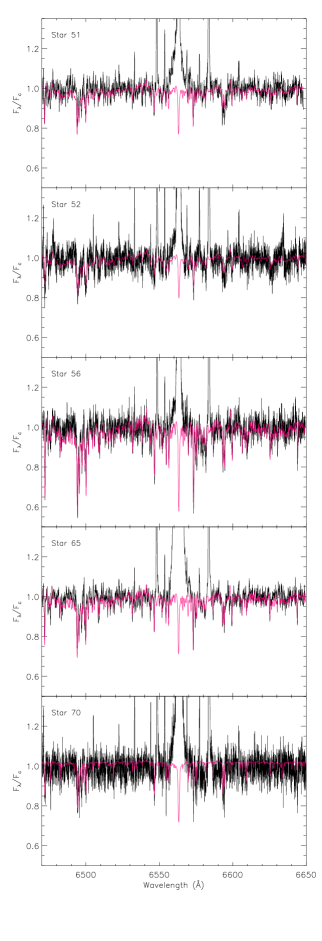
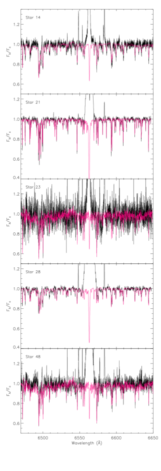
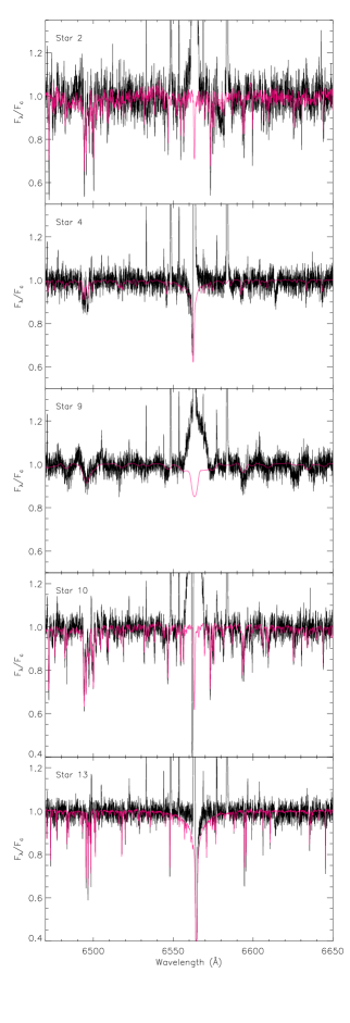
Figure 23: Hectochelle spectra in the H$\alpha$ region of our targets (black lines) with the best template superimposed (thin red lines). The H$\alpha$ emission has been cut in order to display the photospheric absorption lines. The Id number is marked in the top-left corner of each box.

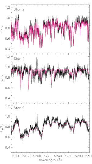
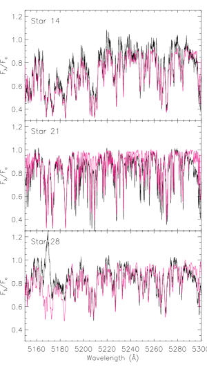
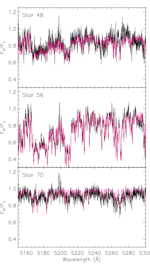
Figure 24: Hectochelle spectra in the Mg i b region of our targets (black lines) with the best template superimposed (thin red lines). The Id number is marked in the top-left corner of each box.

The values of $v\sin i$ and $T_{\rm eff}$, reported in Table 4 for the 15 stars with sufficiently exposed spectra, are the weighted averages of the five best templates. The usual weights, $w_{i}=1/\sigma_{i}^{2}$, where $\sigma_{i}$ are the r.m.s. of each fit, were adopted. The standard errors on $v\sin i$ and $T_{\rm eff}$ are also given in Table 4. In the same table, the spectral types derived by us with ROTFIT and from previous works mainly based on low-resolution spectra are also listed. Some examples of the results of the fitting are shown in Fig. 8. The observed spectra with the fitted templates are displayed in Fig. 23 and Fig. 24 for the H$\alpha$ and the Mg i b spectral regions, respectively.

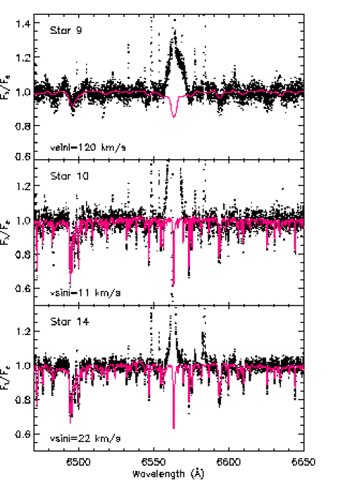
Figure 8: Example of observed Hectochelle spectra (dots) of our targets with the best template superimposed (thin lines). The Id number and the $v\sin i$ value are also marked in each box.

Table 4: Physical parameters and spectral types for the stars with Hectochelle or literature spectra.

Id	2MASS	$P$	$R$	$v\sin i$	$T_{\rm eff}$	Sp. Type	$EW_{H\alpha}^{\rm g}$	$EW_{Li}$	$\sin i$
		(days)	($R_{\sun}$)	(km s-1)	(K)		(Å)	(Å)
2	05352029-0546399	7.751	1.24	7.0$\pm$1.0	3710$\pm$110	M2.5a	7.5		0.864
4	05352007-0545526			30$\pm$5	5720$\pm$100	G2a	0.0
5	05351981-0545409	0.60	1.33			M3.5b
9	05352281-0544428	0.5627	1.98	126$\pm$6	3480$\pm$170	M3a	3.6	0.72c	0.674
10	05352617-0545084	5.816	1.25	11.0$\pm$1.0	4110$\pm$170	K8a	7.0	0.52d	$\simeq 1$
13	05351621-0547201			4.0$\pm$2.0	5800$\pm$200	G1a	0.0
14	05351192-0545379	4.047	1.89	22.5$\pm$1.5	4250$\pm$170	K7a, K8b	3.8	0.41d	0.952
17	05350614-0545311	8.435	1.26			M0b
18	05353222-0544265	12.461	2.16			M3b
19	05352973-0548450	0.605	2.29			K8b
21	05351033-0546335		4.72	12.0$\pm$2.0	4830$\pm$250	K0a	3.9
23	05351011-0548342		0.84	1.0$\pm$0.5	3690$\pm$70	M2.5a	9.0
28	05351423-0543175		3.28	20.0$\pm$1.5	4260$\pm$270	K7a, K7ee	13.7
29	05351236-0543184	8.468	1.87			K7ed
47	05353023-0551169	10.02	1.21			K8b
48	05353047-0549037	7.721	1.04	7.5$\pm$1.5	3830$\pm$220	M2a, M2b	8.6		$\simeq 1$
51	05353316-0547074	2.763	0.92	16.0$\pm$0.5	3690$\pm$100	M3a, M3.5b	2.6		0.949
52	05352930-0545381	1.696	1.03	25.0$\pm$2.0	3740$\pm$90	M2.5a, M3.5b	6.6	0.41c	0.813
56	05353092-0543053	3.80	1.38	13.5$\pm$1.5	3920$\pm$260	M1.5a, M2b	4.9	0.50c	0.734
60	05351643-0542396	4.11	1.40			K5b		0.45c
62	05351715-0541538	2.05	1.18			M5b
65	05345908-0544303		2.07	13.0$\pm$1.5	3990$\pm$260	M1.5a	8.6
70	05350054-0548591		1.50	12.0$\pm$2.0	4600$\pm$500	K5a	8.2
93	05351790-0542340	5.70:	3.33	34f	4775f	K3f			$\simeq 1$

• Present work.

• From Rebull et al. (2000).

• From Stassun et al. (1999).

• From Sicilia-Aguilar et al. (2005).

• From Herbig & Bell (1988).

• From Wolff et al. (2004).

• From Fűrész et al. (2008).

From the values of $v\sin i$, radius ($R$), and rotation period, $P$, reported in Table 4, the inclination of the rotation axis can be estimated as

$$\sin i=\frac{v\sin i\cdot P}{2\pi R}$$ (5)

This parameter is useful for the application of a spot model to the light curves, which is presented in Sect. 6.

6 Spot modelling

The availability of simultaneous light curves from the optical to the NIR allows us to reconstruct roughly the starspot distribution and determine two basic spot parameters, i.e. temperature and dimension. Moreover, hot and cool spots produce a different effect on the $RIJH$ light curves, so that it is possible to discriminate between the two as the main cause for the observed variability (see, e.g. Bouvier & Bertout 1989).

In order to search for a unique solution for the multi-band light curves, we used MACULA, a spot model code developed by us in the IDL environment (Frasca et al. 2005). The model assumes circular dark (cool) or bright (hot) spots on the surface of a spherical limb-darkened star. The linear limb-darkening coefficients for $RIJHK$ bands are from Claret (2000), who calculated them for a grid of Phoenix NextGen models.

Frasca et al. (2005) have shown that two circular spots are sufficient to reproduce the general shape of light curves of spotted stars without introducing too many free parameters.

The flux contrast ($F_{\rm sp}/F_{\rm ph}$) can be evaluated through the Planck spectral energy distribution, the ATLAS9 (Kurucz 1993) and PHOENIX NextGen (Hauschildt et al. 1999) atmosphere models. Frasca et al. (2005) demonstrated that both ATLAS9 and NextGen provide values of the spot temperature ($T_{\rm sp}$) and area coverage ($A_{\rm rel}$) that are in close agreement, while the black-body assumption for the SED leads to underestimate the spot temperature. In the present work, we have preferred the NextGen flux ratios because they can go down to a temperature of 1700 K, while the minimum temperature for ATLAS9 fluxes is 3500 K, which is close to the photospheric temperature of the coolest stars in our sample. For this purpose, we integrated the NextGen spectra, weighted with the transmission curves of the REM filters.

We applied our code only to the six stars with the highest-quality light curves in at least three photometric bands. For three of them with Hectochelle spectra, namely #9, #10, and #14, we have an estimate of the inclination of the rotation axis through Eq. 5. For the remaining stars to which we applied the spot modelling (#11, #17, and #18) we adopted a value of $i=70\degr$, which is a reasonable choice given the rather large amplitudes of their light curves. For each star, we started to fit the light curve in a reference band (usually $I$) with a 2-spot model at a fixed temperature (normally $T_{\rm sp}/T_{\rm ph}\,=\,$ 0.80), and found the geometrical parameters of the spots (longitudes and latitudes) as well as their area by minimizing the $\chi^{2}$. Then, we fixed the spot positions and, for a few fixed values of the temperature ratio ($T_{\rm sp}/T_{\rm ph}$), we let the spot dimensions to vary, searching for the value of spot area which minimizes the $\chi^{2}$ of the fit for the given value of $T_{\rm sp}/T_{\rm ph}$. As already found by Frasca et al. (2005), the $\chi^{2}$ does not vary significantly for large intervals of $T_{\rm sp}/T_{\rm ph}$, so that several models in the solution grid, for a given passband, are fitting the light curve with the same accuracy. Only the use of at least two diagnostics permits to remove the degeneracy of $T_{\rm sp}$ and area in the space of the parameters.

The grids of solutions for different bands allow to define the ranges of values for the spot temperature and area as those for which all the curves are well fitted within the errors.

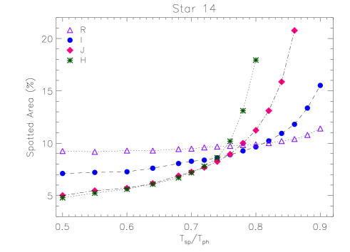
Figure 9: Grids of solutions of $RIJH$ light curves for star #14. Each pass-band is represented by a different symbol.

The results of the solution grids for the $RIJH$ light curves of star #14, for which we found $i=70\degr$ (see Table 5), are displayed in Fig. 9, where the percent spotted area (in units of star surface) versus the fractional spot temperature $T_{\rm sp}/T_{\rm ph}$ is plotted. The figure shows the different behaviour of the $RIJH$ solution grids, and the rather small region in the plane $T_{\rm sp}/T_{\rm ph}$–$A_{\rm rel}$ were the intersection of the four solution grids occurs. This allows us to assert that the fractional spot temperature is $T_{\rm sp}/T_{\rm ph}\simeq 0.76\pm 0.04$, i.e. a spot temperature in between 3000 and 3400 K, and a spotted area in the range 7–9%. In Fig. 10, the observed $RIJH$ light curves and the simultaneous solution provided by MACULA are displayed together with a map of the spotted photosphere, as seen at the rotational phase of maximum spot visibility.

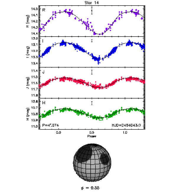
Figure 10: Observed (dots) and synthetic (full lines) $R$, $I$, $J$, and $H$ light curves of star #14. The mean error-bar is also displayed in the upper mid part of each box. A schematic map of the starspot distribution, as seen at the phase of maximum spot visibility, is also shown. The inclination of the rotation axis, as derived from Eq. 5, is $i=70\degr$.

Similar results are obtained for star #10 ($i\simeq 90\degr$), for which the grids of solutions intersect each other for values of $T_{\rm sp}/T_{\rm ph}\simeq 0.76\pm 0.02$ (Fig. 11). We also tried with hot spots, but the solution grids in different bands do not intersect, ruling out accretion as the cause of the observed modulation. This is a remarkable result because star #10 displays the characteristics of a cTTS, such as the very strong and broad H$\alpha$ emission (Fűrész et al. 2008) and the mid-IR excess (Fig. 5) which testifies the presence of a conspicuous accretion disc. It seems that cool photospheric spots, indicative of strong magnetic activity, are presumably the main responsible for the observed variability.

Figure 11: Grids of solutions of $RIJH$ light curves for star #10. Different symbols have been used for each pass-band.

However, superimposed to the rotational modulation, additional “fluctuations” larger than typical errors are clearly visible in the $RIJH$ light curves of star #10 (Fig. 12). These features appear to be correlated in the different bands. This kind of variability was already observed in some young stars in Orion by, e.g., Carpenter et al. (2001) and could be ascribed to intrinsic variability due to accretion.

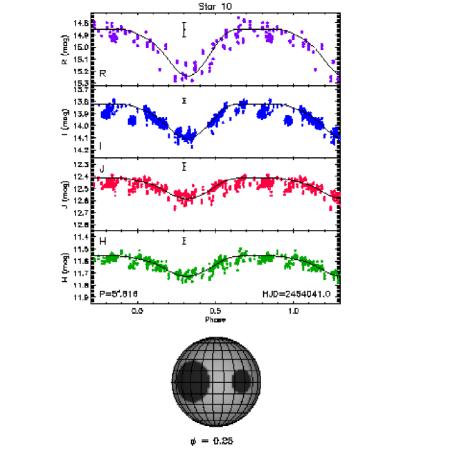
Figure 12: Observed (dots) and synthetic (full lines) $R$, $I$, $J$, and $H$ light curves of star #10. The mean error-bar is also displayed in the upper mid part of each box. A schematic map of the starspot distribution, as seen at the phase of maximum spot visibility, is also shown. The inclination of the rotation axis, as derived from Eq. 5, is $i=90\degr$.

The last star with known inclination ($i=45\degr$) analyzed with MACULA for the determination of spot parameters is #9. This star displays fairly good light curves in $RIJH$ bands, although with rather low amplitudes, and is a very interesting case because of its very short rotation period. As seen in Fig. 13, the intersection of the solution grids occurs for larger values of fractional spot temperature compared to the previous stars. We found $T_{\rm sp}/T_{\rm ph}\simeq 0.93\pm 0.03$, which corresponds to a temperature difference $\Delta T\simeq 270\pm 100$ K.

Figure 13: Grids of solutions of $RIJH$ light curves for star #9. Different symbols have been used for each pass-band.

Spot temperatures of a few hundreds Kelvin degrees cooler than the surrounding photosphere have been found in very active and fast-rotating cool stars (see, e.g., Oláh & Kövári 1997; Berdyugina 2005). We remark that we cannot assess if the spots are really uniform and warmer than in the other Orion stars analyzed by us or if there is a mixture of regions with different temperatures. In this case, warmer areas (analogous to the sunspot penumbrae) could be dominating. The lower temperature could be also the effect of the simultaneous presence in the same area of cool spots and bright white-light faculae. There is no way, with the present photometric data, to further investigate this point. A simultaneous light curve in the near-UV could be very helpful to detect bright faculae which should have a much higher contrast at shorter wavelengths.

In Fig. 14, the observed $RIJH$ light curves and the simultaneous solution provided by MACULA are displayed together with a map of the spotted photosphere, as seen at the rotational phase of maximum spot visibility.

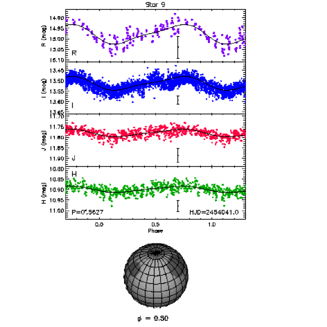
Figure 14: Observed (dots) and synthetic (full lines) $R$, $I$, $J$, and $H$ light curves of star #9. The mean error-bar is also displayed in the lower mid part of each box. A schematic map of the starspot distribution, as seen at the phase of maximum spot visibility, is also shown. The inclination of the rotation axis, as derived from Eq. 5, is $i=45\degr$.

For the star #17, we assumed an inclination $i=70\degr$ and obtained a spot temperature of $T_{\rm sp}/T_{\rm ph}\simeq 0.71\pm 0.03$ from the solution grids in the $RIJH$ bands displayed in Fig. 15. This star shows spot properties similar to #14 and #10.

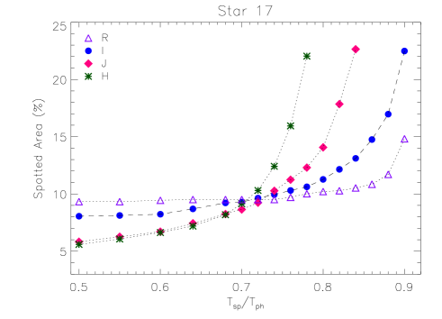
Figure 15: Grids of solutions of $RIJH$ light curves for star #17. Different symbols have been used for each pass-band.

In Fig. 16, the observed $RIJH$ light curves and the simultaneous solution provided by MACULA are displayed together with a map of the spotted photosphere, as seen at the rotational phase of maximum spot visibility.

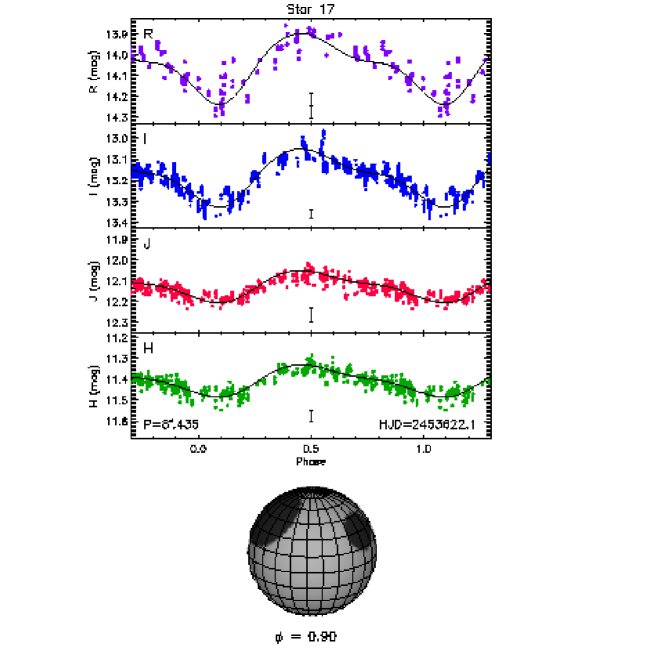
Figure 16: Observed (dots) and synthetic (full lines) $R$, $I$, $J$, and $H$ light curves of star #17. The mean error-bar is also displayed in the lower mid part of each box. A schematic map of the starspot distribution, as seen at the phase of maximum spot visibility, is also shown. An inclination of the rotation axis $i=70\degr$ was adopted.

We also tried simultaneous solutions of the $RIJH$ bands for star #18. We were able to fit the individual light curves with a model with two cool spots but the grids of solutions for different bands do not show any intersection, as seen in the top panel of Fig. 17. This is due to the strong decrease of the amplitude of the light curves that goes from 0$\aas@@fstack{m}$225 to 0$\aas@@fstack{m}$110 from $R$ to $I$ and becomes as low as 0$\aas@@fstack{m}$055 in $J$ and $H$ bands. There is no value of $T_{\rm sp}/T_{\rm ph}$ that allows such a rapid amplitude decrease. As shown by Bouvier & Bertout (1989) for DF Tau, a steep decrease of the modulation amplitude with the increasing wavelength can be reproduced only with hot spots. Thus, we tried to model the light curves with hot spots and found intersection of all the solution grids for a value of $T_{\rm sp}/T_{\rm ph}=1.10\pm 0.02$ corresponding to spots 360$\pm 70$ K hotter than the surrounding photosphere. This does not imply that cool spots are not present on the photosphere of this star, but the main responsible for the observed variations are hot spots.

Figure 17: Top) Grids of cool-spot solutions of $RIJH$ light curves for star #18. Different symbols have been used for each pass-band. Bottom) Grids of hot-spot solutions.

We cannot state whether these features are tied to accretion because we have neither Hectochelle spectra nor mid-IR photometry, but the relatively long rotation period ($P_{\rm rot}\simeq 12.5$ days) and the position on the HR diagram are consistent with a very young disc-locked object still in an active phase of mass accretion.

The $RIJH$ light curves and the simultaneous solution provided by MACULA are displayed together with a map of the hot spots in Fig. 18.

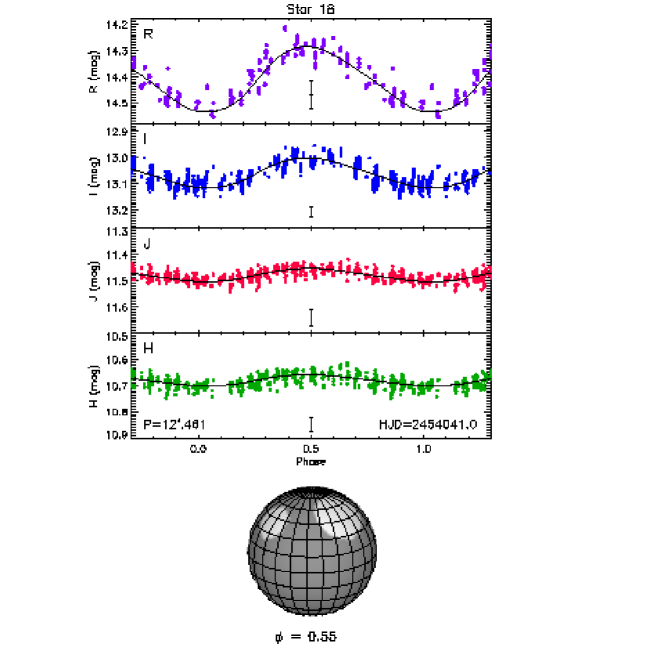
Figure 18: Observed (dots) and synthetic (full lines) $R$, $I$, $J$, and $H$ light curves of star #18. The mean error-bar is also displayed in the lower mid part of each box. A schematic map of the hot-spot distribution, as seen at the phase of maximum spot visibility, is also shown. An inclination of the rotation axis $i=70\degr$ was adopted.

The last object for which we attempted to model the rotational modulation with MACULA is star #11, the one with the largest modulation amplitude in our sample. This object is very red and too faint in the $R$ band for obtaining a suitable light curve. Only an indication of a modulation amplitude $\Delta R\simeq 0\aas@@fstack{m}97$ can be derived. The $I$, $J$, and $H$ curves are instead fully usable. We initially tried with cool spots and found solutions with very large active regions, covering a large fraction of a stellar hemisphere, as expected for getting variation amplitudes of about 1 magnitude. Anyway, as seen in the top panel of Fig. 19, there is no intersection between the grids for different bands. We also tried with hot spots without success (Fig. 19, bottom panel). This result is not surprising if we consider that the amplitude of the light curves has a reverse trend, as a function of wavelength, compared to the rotational modulation produced by cool or hot spots for the other sources. For star #11, the modulation amplitude slightly increases with the central wavelength of the band. A possible explanation for this behaviour is that the main source of variation is not the stellar photosphere but the accretion disc from which most of the NIR flux originates (see Fig. 5). Inhomogeneities/condensations in the disc could give rise to wavelength-independent or increasing amplitudes, depending on the ratio of stellar to disc luminosity at the wavelength of observation. Indeed, star #11 is the object with the largest IR excess in our sample.

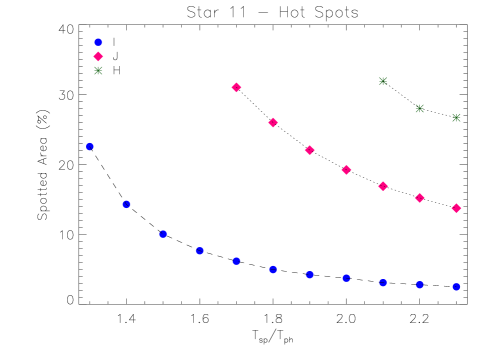
Figure 19: Top) Grids of cool-spot solutions of $RIJH$ light curves for star #11. Different symbols have been used for each pass-band. Bottom) Grids of hot-spot solutions.

7 Discussion

Having detected rotation periods for 29 stars in a field flanking the ONC and derived spot parameters for a few of them, we now shortly discuss our results accounting for the evolutionary status of the investigated sources and the evidences of active accretion and circumstellar discs for some of them. Moreover, the characteristics of the strong flare of star #19 (2MASS J05352973-0548450) are discussed in some details.

As shown in Table 3, forty-three stars are likely members (either photometric and/or kinematic) of the Orion cloud, and their positions in the HR diagram appear consistent with those of PMS stars. Furthermore, our analysis of the SEDs reveals that five of these stars (namely, #10, #11, #59, #61, and #93) have significant IR excesses, signature of circumstellar discs. Star #10 was reported by Sicilia-Aguilar et al. (2005) as a possible cTTS. This classification would be consistent with the IR excess of the object. Stars #59 and #61 exhibit, beside to the NIR excess, erratic photometric variations, quite common in T Tauri stars.

7.1 Rotation period distribution

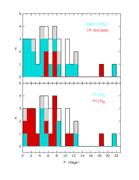
Figure 20: The two panels show the distributions of rotation periods for stars in the REM field (thick line), and for the subsample classified as Orion members (hatched area). The upper panel highlights the stars younger than 10 Myr (light-grey/cyan shaded area) and the objects with NIR excess (dark-grey/red shaded area). The lower panel highlights the members with masses respectively less than (dark-grey/red) and higher than (light-grey/cyan) 1 M_⊙.

The distribution of rotation periods is shown in Fig. 20. From the upper panel, we note that the majority of the objects with detected period are classified as Orion members. The latter are dominated by stars younger than 10 Myr, among which five objects with significant NIR excess are found. Notably, none of these stars with NIR excess has a rotation period shorter than 5 days, in agreement with the hypothesis that the angular momentum of the stars is moderated by interaction with the disc. The lower panel shows instead the two subsamples with masses less than and higher than 1 $M_{\odot}$, respectively, but we do not see any obvious dependency upon mass. The poor statistics prevent us to unambiguously distinguish the bimodal distribution with peaks near 2 and 8 days clearly displayed by ONC members (Herbst et al. 2002).

7.2 Spot properties

In most cases, the amplitudes of the modulation detected in different photometric bands decrease at longer wavelengths, with a wavelength dependency that is consistent with the presence of cool photospheric spots, except for star #18, whose behaviour can only be reproduced with hot spots. Two stars (namely, #11, and #91) show instead either increasing or almost invariant amplitudes at longer wavelengths. Star #11, which exhibits the broadest modulation in our sample, shows light-curve amplitudes that increase from 0.85 mag in $V$ to 1.25 mag in $J$ and slightly decrease in $H$ and $K$. This star also shows a remarkable excess emission in the mid-IR, hence the cause of variability might reside in the inner circumstellar disc (e.g., possible disc inhomogeneities/instabilities). Indeed, the observed modulation in the $IJH$ bands could not be modelled neither with cool nor with hot starspots. Star #91, with relatively small photometric variations, has almost invariant light-curve amplitudes. In contrast, star #10, which displays the typical signatures of a cTTS, exhibits modulation amplitudes that decrease systematically from $R$ to $H$ and are well reproduced by cool spots with $T_{\rm sp}/T_{\rm ph}\simeq 0.76$.

For five stars with fairly good light curves in the $RIJH$ bands we could find the spot parameters from the simultaneous solution of the multi-band light curves (Sect. 6). These data are summarized in Table 5. Apart from star #18, we found cool spots. It is interesting to note that the temperature of the cool spots is nearly the same ($T_{\rm sp}\simeq 3100$ K) for all the four stars regardless of the photospheric temperature. This average value is noticeably lower than sunspot umbrae ($T\approx 3800$ K). However, it is not easy to define the best parameter describing the blocking effect on energy convective transport produced by the spot magnetic fields. For a more meaningful comparison, the temperature ratio, $T_{\rm sp}/T_{\rm ph}$, or the temperature difference, $\Delta T=T_{\rm ph}-T_{\rm sp}$, should be adopted. As seen in Table 5, for the three stars with fairly long rotation periods (#10, #14, and #17) $\Delta T$ is in the range 1000–1300 K, i.e. smaller than sunspot umbrae but slightly larger than values of 400–900 K found for the giant and sub-giants components of RS CVn binaries adopting a similar approach (Frasca et al. 2005, 2008). Conversely, the spotted area (8–10% of the star surface) is smaller, on average, than that found by Frasca et al. (2005, 2008) for RS CVn stars ($A_{\rm rel}$=11–18%). Our results are in agreement with Bouvier & Bertout (1989), which, from multi-band photometry, find cool spots in T Tau stars with temperature mostly in the range 700–1200 K and filling factors ranging from about 5% to 10%. The difference between these Orion population stars and the Sun is likely due to the clear tendency for spots to have a larger contrast with respect to the photosphere in hotter stars (Berdyugina 2005, and references therein). However, the higher temperature contrast compared to RS CVn stars is not due to this effect because our PMS stars have $T_{\rm eff}$ in the range 4100–4400 K, hence cooler than the aforementioned RS CVn components ($T_{\rm eff}\sim$ 4600–4900 K). The different internal structure of the fully convective PMS stars, compared to sub-giant stars, could be responsible for such behaviour. The much lower $\Delta T$ found for star #9 is in line with its lower effective temperature but could also be tied to its very high rotation rate.

Table 5: Spot parameters^∗.

Id	$i$	$R_{1}$	$Lon_{1}$	$Lat_{1}$	$R_{2}$	$Lon_{2}$	$Lat_{2}$	$T_{\rm sp}/T_{\rm ph}$	$T_{\rm sp}$	$\Delta T$	$A_{\rm rel}$
	($\degr$)	($\degr$)	($\degr$)	($\degr$)	($\degr$)	($\degr$)	($\degr$)		(K)	(K)	(%)
#9	45	20.4	42	45	13.3	170	40	0.92$\pm$0.03	3240$\pm$100	270	5.0${}^{+3.5}_{-1.5}$
#10	90	27.6	126	0	15.6	55	0	0.76$\pm$0.02	3120$\pm$ 80	990	7.5$\pm$0.5
#14	70	29.3	240	45	18.2	150	25	0.76$\pm$0.04	3230$\pm$170	1020	8.0$\pm$1
#17	70	31.6	33	45	18.3	265	30	0.71$\pm$0.03	3120$\pm$130	1280	9.5$\pm$1.5
#18	70	23.6	155	50	16.0	252	40	1.10$\pm$0.02	3960$\pm$ 70	$-$360	6.0$\pm$1

^∗ $R_{1}$, $Lon_{1}$, and $Lat_{1}$ are radius, longitude, and latitude of the larger spot. $R_{2}$, $Lon_{2}$, and $Lat_{2}$ are the same for the smaller spot. The spot temperature is the same for both spots and is expressed in units of the photospheric temperature, $T_{\rm sp}/T_{\rm ph}$, as well as in Kelvin degrees. The difference $\Delta T=T_{\rm ph}-T_{\rm sp}$ is also listed. The total spot area, $A_{\rm rel}$, is expressed in percent units of the star surface.

7.3 Flare events in 2MASS J05352973-0548450 and 2MASS J05352550-0545448

Star # 19 (2MASS J05352973-0548450) is a known variable (V498 Ori), already classified both as a flare star (Parenago 2078), and an emission-line star (Haro 4-365, PaCh 274, Kiso A-0976 174).

Here we report the serendipitous detection, on the 7th of December 2006 at 4:41 UT, of a remarkable flare event from star # 19 in the $I$ band (see Fig. 3). The peak amplitude ($\Delta\,I\simeq 0.3$ mag) and the duration of the flare are comparable to those observed by Scholz & Eislöffel (2005) in a rapidly rotating ($P=0.61$ days), very low-mass (0.09 $M_{\sun}$) member of the $\epsilon$ Ori cluster. Though, we were able, thanks to the prolonged and dense temporal sampling of our $I$-band observations, to follow the entire event and resolve both the rise and decay phases.

The luminosity in the $I$ band at the flare peak, $L_{I}^{\rm peak}$, can be evaluated from the equation

$$L_{I}=4\pi d^{2}\cdot 10^{-0.4(I-A_{I})}F_{I}W\mathrm{(erg\,s^{-1})}$$ (6)

where $d=414$ pc is the distance to the star, $I$ is the apparent magnitude of the star, $A_{I}=0.58A_{V}$ is the extinction in the $I$ band, $F_{I}=1.196\times 10^{-9}$ erg cm^-2 s^-1Å^-1 (Lamla 1982) is the Earth flux (outside the atmosphere) in the $I$ band from a zero-magnitude star, and $W\approx 1000$ Å  is the $I$ band-width. We find a flare peak luminosity $L_{I}^{\rm peak}\simeq 1.7\cdot 10^{32}$ erg s^-1. The stellar luminosity before the flare $L_{I_{0}}\simeq 5.3\cdot 10^{32}$ erg s^-1, corresponding to a magnitude $I_{0}=11\aas@@fstack{m}91$, has been subtracted.

The energy released during the flare in the $I$ band, $E_{I}\simeq 2.7\cdot 10^{35}$ erg, was computed by integrating the excess luminosity (over the pre-flare level) all along the duration of the flare. The flare results to be a very powerful one.

We estimated the coverage factor of the flaring area following the guidelines of Hawley et al. (1995). They showed that the continuum emission from the near-UV to the R band of strong flares in dMe stars is well reproduced by a black-body spectrum with a temperature of $\sim$ 9000 K. This is also in agreement with the findings of Machado & Rust (1974) for the continuum emission in a solar flare that they find consistent with thermal emission from electrons at $T_{e}=8500\pm 500$ K in the upper photosphere. According to Eq. 3.1 of Hawley et al. (1995), one can estimate the temperature of the flaring region and the area coverage at the flare peak with observations in at least two bands. From $I$ and $J$ light curves of the flare of V498 Ori we could derive both parameters. Given the relatively large errors of the $J$ magnitudes ($\sim 0.03$ mag) compared to the flare intensification in the $J$ band ($\Delta J\sim 0.09$ mag), we preferred to fix the temperature to $T_{\rm flare}=9000$ K and deduced an area coverage $X$ of about 14%. This is much larger than the typical values of $\sim 0.01$% found by Hawley et al. (1995) in dMe stars. An estimate of the total flare optical luminosity is then given by $L_{\rm opt}=X\cdot 4\pi R^{2}\sigma T_{\rm flare}^{4}\sim 1.6\cdot 10^{34}$ erg s^-1 and the optical flare energy turns out to be $\sim 6\cdot 10^{36}$ erg. These values are about 3 orders of magnitude larger than those derived by Hawley et al. (1995) for an optical flare of the dMe star AD~Leo.

Other parameters characterizing the flare are the rise and decay time-scales. We fitted the rise and decay phase of the flare light curve with an exponential function of the form

$$I(t)=\Delta Ie^{[(t-t_{\rm peak})/\tau)]}+I_{0}$$ (7)

We found as rise and decay e-folding times the values $\tau_{r}\simeq 2.5$ min and $\tau_{d}\simeq 24.9$ min, respectively.

We applied the same analysis to the flare observed on the 10th of December 2006 at 1:30 UT on star # 11 (2MASS J05352550-0545448 = NR~Ori) in the $I$ band (see Fig. 21). The peak amplitude, $\Delta\,I\simeq 0.85$ mag, was higher than in the previous event of star # 19 but the duration of the flare ($\simeq$ 110 minutes) was nearly the same. We found rise and decay e-folding times of $\tau_{r}\simeq 6$ min and $\tau_{d}\simeq 59$ min, respectively. No flux intensification was observed in the $J$ band. The peak luminosty and the energy released in the $I$ band are $L_{I}^{\rm peak}\simeq 1.4\cdot 10^{31}$ erg s^-1 and $E_{I}\simeq 6.4\cdot 10^{34}$ erg, i.e. smaller than those derived for the flare on star # 19, notwithstanding the huge $I$-flux intensification. This is due to contrast reasons, being star # 11 intrinsically much fainter than star # 19. Assuming a flare temperature $T_{\rm flare}=9000$ K, we found an area coverage factor $X\simeq$ 3%. The total flare luminosty and the energy released at optical wavelengths, calculated as for star # 19, are $L_{\rm opt}\sim 9.7\cdot 10^{32}$ erg s^-1 and $E_{\rm opt}\sim 4.4\cdot 10^{34}$ erg s^-1.

We can finally attempt a very rough estimate of the flare frequency among the stars in the REM field that we classify as members and likely members of the young Orion population, using the time interval covered by observations ($\approx 50$ hours) and the number of objects and found a value of the order of $8\times 10^{-4}{\rm h}^{-1}$.

8 Conclusions

We presented the results of an intensive photometric monitoring of a 10$\arcmin\times 10\arcmin$ field flanking the Orion Nebula Cluster (ONC) conducted during three consecutive months. The main results of our work can be summarized as follows:

• We detected rotation periods for 29 stars, spanning from about 0.6 to 20 days, sixteen of which are new periodic variables. Thanks to the relatively long time-baseline we measured the periods with sufficient accuracy ($\Delta P/P<2\%$) also for the slowest rotators. We remark that none of the stars with NIR excess has a rotation period shorter than 5 days, in agreement with the hypothesis that the angular momentum of the stars is moderated by interaction with the disc.

• The analysis of the spectral energy distribution and, for some stars, the high-resolution spectra provided us with $T_{\rm eff}$ and luminosity, and that allowed us to construct the HR diagram of these stars. We could then assign a photometric membership to the objects by a comparison with PMS evolutionary tracks and derive masses and ages. The majority of the objects with detected period are classified as Orion members and result to be younger than 10 Myr.

• Our spot modelling code enabled us to derive the starspot properties for five of these star, based on the simultaneous analysis of the light curves in several optical and NIR bands. For one of these, the light curves could only be modelled with hot spots, which are likely related to magnetospheric accretion. For three stars with $T_{\rm eff}$ in the range 4100–4400 K and rotation periods between 4 and 8 days we found cool spots with $\Delta T=T_{\rm ph}-T_{\rm sp}$ in the range 1000–1300 K, i.e. larger, on average, than $\Delta T$ typically found for the sub-giant and giant components of RS CVn systems. Conversely, the spotted area (8–10% of the star surface) is smaller. These differences could be due to the fully convective internal structure of PMS stars which gives rise to a different dynamo action. For the cool ($T_{\rm eff}\simeq 3500$ K) and ultra-fast ($P\simeq 0.56$ days) star #9, a smaller spot contrast ($\Delta T\simeq 270$ K) is found. This could be due both to the lower effective temperature and the high rotation rate.

  For the star with the highest modulation amplitudes (star #11), which also displays a remarkable near- and mid-IR excess, the light curves were not consistent neither with hot nor with cool spots. We suggest that the flux modulation could be produced by inhomogeneities of the circumstellar disk.

• A very strong flare was detected on star #19 (V498 Ori) in the $I$ band. The temporal evolution of the event was fully resolved and we evaluated the rise and decay e-folding times as $\tau_{r}\simeq 2.5$ min and $\tau_{d}\simeq 24.9$  min, respectively. We estimated an energy released in the $I$ band of nearly $3\cdot 10^{35}$ erg and a 20 times higher energy released in the optical continuum. Another strong flare, which released an energy of about $6\cdot 10^{34}$ erg in the $I$ band, was observed on star # 11 (NR~Ori), which is cooler and less massive than star # 19 and displays the broadest modulation and a strong infrared excess.

Table 6: Standard $VRIJHK^{\prime}$ magnitudes of all the sources.

Id 2MASS $V$ err $R$ err $I$ err $J$ err $H$ err $K$ err [3.6] [4.5] [5.8] [8.0] (mag) (mag) (mag) (mag) (mag) (mag) (mag) (mag) (mag) (mag) (mag) (mag) (mag) (mag) (mag) (mag) 1 05352184-0546085 … … 19.21 0.43 17.28 0.17 14.71 0.06 14.09 0.05 13.75 0.12 … … … … 2 05352029-0546399 16.30 0.08 15.13 0.06 13.89 0.02 12.46 0.03 11.76 0.03 11.57 0.05 … … … … 3 05352021-0546510 15.72 0.08 14.63 0.06 13.39 0.02 12.01 0.03 11.27 0.03 11.07 0.04 … … … … 4 05352007-0545526 16.12 0.08 15.23 0.06 14.38 0.02 12.99 0.03 12.37 0.03 12.13 0.05 … … … … 5 05351981-0545409 16.92 0.07 15.73 0.06 14.26 0.02 12.70 0.03 12.03 0.03 11.80 0.05 … … … … 6 05351903-0546163 16.26 0.08 15.18 0.06 13.81 0.02 12.36 0.03 11.64 0.03 11.43 0.05 … … … … 7 05351924-0547012 18.60 0.11 17.03 0.09 15.26 0.03 13.51 0.04 12.92 0.03 12.65 0.06 … … … … 8 05351950-0547457 16.72 0.08 15.57 0.06 14.27 0.02 12.93 0.03 12.22 0.03 12.03 0.05 … … … … 9 05352281-0544428 16.31 0.08 14.97 0.06 13.52 0.02 11.78 0.03 10.90 0.03 10.62 0.04 10.45 10.49 10.50 10.43 10 05352617-0545084 16.05 0.08 14.99 0.06 13.97 0.02 12.49 0.03 11.63 0.03 11.27 0.05 10.55 10.23 9.72 8.96 11 05352550-0545448 16.80 0.07 16.33 0.08 15.46 0.04 13.45 0.04 12.10 0.03 11.10 0.05 9.93 9.56 9.22 8.39 12 05351695-0545558 17.17 0.07 16.01 0.06 14.21 0.02 12.28 0.03 11.59 0.03 11.28 0.05 … … … … 13 05351621-0547201 15.89 0.08 14.97 0.06 14.07 0.02 12.68 0.03 11.99 0.03 11.77 0.05 … … … … 14 05351192-0545379 15.23 0.08 14.21 0.06 13.19 0.02 11.60 0.03 10.80 0.03 10.55 0.04 10.27 10.37 10.29 10.50 15 05351290-0545376 18.43 0.16 17.10 0.09 15.40 0.04 13.31 0.04 12.53 0.03 12.17 0.05 … … … … 16 05351797-0549375 15.26 0.08 14.35 0.06 13.13 0.02 11.94 0.03 11.23 0.03 11.04 0.04 … … … … 17 05350614-0545311 15.02 0.09 14.06 0.06 13.18 0.02 12.14 0.03 11.42 0.03 11.25 0.05 11.09 11.18 11.25 10.97 18 05353222-0544265 15.62 0.08 14.40 0.06 13.06 0.02 11.48 0.03 10.68 0.03 10.42 0.04 … … … … 19 05352973-0548450 13.59 0.09 12.73 0.06 11.88 0.02 10.75 0.03 10.07 0.03 9.90 0.05 … … … … 20 05350738-0548010 17.50 0.26 16.86 0.08 14.81 0.03 12.45 0.03 11.41 0.03 10.99 0.05 … … … … 21 05351033-0546335 12.88 0.09 11.91 0.06 11.06 0.02 9.56 0.04 9.20 0.03 8.47 0.05 … … … … 22 05351205-0547296 … … 18.48 0.23 16.41 0.08 14.08 0.04 13.31 0.04 12.91 0.07 … … … … 23 05351011-0548342 17.07 0.07 16.02 0.07 14.56 0.03 13.27 0.03 12.60 0.03 12.38 0.05 … … … … 24 05351400-0549362 … … … … … … 8.66 0.06 8.64 0.03 8.73 0.05 … … … … 25 05351493-0549348 13.97 0.08 13.80 0.05 13.34 0.03 12.03 0.03 11.38 0.03 11.19 0.05 … … … … 26 05352616-0548166 … … … … … … 9.39 0.03 9.27 0.03 9.27 0.05 … … … … 27 05352637-0544340 17.65 0.08 16.98 0.09 15.45 0.04 13.88 0.04 13.20 0.03 12.85 0.07 … … … … 28 05351423-0543175 13.50 0.09 12.71 0.06 11.84 0.02 10.41 0.03 9.56 0.03 9.03 0.05 … … … … 29 05351236-0543184 13.85 0.09 12.98 0.06 12.23 0.02 11.19 0.03 10.46 0.03 10.25 0.05 … … … … 30 05351146-0544183 … … 17.65 0.12 15.82 0.05 13.80 0.04 13.09 0.03 12.76 0.06 … … … … 31 05350575-0544001 16.63 0.08 15.48 0.06 14.09 0.02 12.83 0.03 12.12 0.03 11.87 0.05 … … … … 32 05350567-0543046 … … 17.59 0.13 15.71 0.05 14.27 0.05 13.62 0.05 13.51 0.11 … … … … 33 05350486-0544267 … … 18.97 0.41 17.85 0.32 15.20 0.08 13.57 0.05 12.69 0.06 … … … … 34 05350278-0544429 … … … … … … 13.81 0.04 13.15 0.04 12.87 0.07 … … … … 35 05350303-0545333 18.63b 0.05 … … 15.46b 0.02 12.83 0.03 11.70 0.03 11.24 0.04 … … … … 36 05350421-0545469 … … … … … … 14.12 0.05 13.03 0.04 12.62 0.06 … … … … 37 05350215-0547200 … … … … … … 14.54 0.05 13.49 0.04 13.08 0.08 … … … … 38 05350176-0548140 … … … … … … 14.65 0.06 13.42 0.04 12.70 0.06 … … … … 39 05350406-0548540 17.12 0.07 16.01 0.07 14.50 0.03 13.40 0.04 12.70 0.03 12.53 0.06 … … … … 40 05350627-0549021 … … … … 18.48a 0.51 14.33 0.05 12.59 0.03 11.70 0.05 … … … … 41 05350825-0550003 16.31 0.08 15.35 0.06 13.99 0.02 12.90 0.03 12.19 0.03 12.03 0.05 … … … … 42 05351088-0549485 … … 17.45 0.12 15.56 0.05 14.10 0.04 13.49 0.04 13.33 0.09 … … … … 43 05351602-0550448 … … … … … … 13.31 0.04 12.44 0.03 12.05 0.05 … … … … 44 05351473-0551040 … … … … … … 12.59 0.03 11.36 0.03 10.78 0.04 … … … … 45 05352193-0551071 … … … … … … 9.72 0.03 9.32 0.03 9.26 0.04 … … … … 46 05352538-0551087 … … … … … … 8.83 0.04 8.52 0.03 8.36 0.04 … … … … 47 05353023-0551169 14.76c 0.05 … … 13.31d 0.02 12.10 0.03 11.39 0.03 11.22 0.05 11.13 11.03 11.11 11.01 48 05353047-0549037 16.50 0.08 15.46 0.06 14.22 0.03 12.89 0.04 12.06 0.03 11.76 0.05 … … … … 49 05353294-0549326 … … 18.01 0.17 16.21 0.08 14.56 0.05 13.77 0.04 13.49 0.10 … … … … 50 05353385-0548211 … … 17.65 0.13 16.22 0.08 14.24 0.05 13.29 0.04 12.98 0.07 … … … … 51 05353316-0547074 16.72 0.08 15.69 0.06 14.35 0.02 13.08 0.03 12.37 0.03 12.17 0.05 11.90 11.72 11.58 10.94 52 05352930-0545381 16.91 0.07 15.80 0.06 14.37 0.02 12.91 0.03 12.23 0.03 12.02 0.05 … … … … 53 05353372-0546162 16.98 0.07 16.03 0.07 14.63 0.03 13.33 0.03 12.63 0.03 12.42 0.06 … … … … 54 05353266-0545284 … … 19.34 0.59 16.98 0.14 14.33 0.05 13.50 0.04 12.98 0.09 … … … … 55 05353229-0544060 17.21 0.07 16.01 0.07 14.60 0.03 13.24 0.03 12.54 0.03 12.34 0.05 … … … …

Table 6: Continued.

Id 2MASS $V$ err $R$ err $I$ err $J$ err $H$ err $K$ err [3.6] [4.5] [5.8] [8.0] (mag) (mag) (mag) (mag) (mag) (mag) (mag) (mag) (mag) (mag) (mag) (mag) (mag) (mag) (mag) (mag) 56 05353092-0543053 15.27 0.08 14.23 0.06 13.18 0.02 12.06 0.03 11.32 0.03 11.14 0.05 … … … … 57 05352765-0542551 15.89 0.08 14.78 0.06 13.72 0.02 11.98 0.03 10.97 0.03 10.56 0.05 … … … … 58 05352634-0543364 … … 18.17 0.20 16.23 0.07 14.20 0.04 13.56 0.04 13.29 0.09 … … … … 59 05352125-0542123 15.95 0.08 14.99 0.06 13.84 0.02 12.29 0.04 11.45 0.03 10.94 0.05 10.11 9.84 9.45 8.46 60 05351643-0542396 13.58 0.09 12.84 0.06 12.32 0.02 11.51 0.03 10.87 0.03 10.75 0.05 10.70 10.89 10.75 10.48 61 05351734-0542145 16.49 0.08 15.41 0.06 14.08 0.02 12.46 0.04 11.56 0.03 11.00 0.05 9.85 9.12 8.67 7.55 62 05351715-0541538 17.83 0.06 16.44 0.08 14.73 0.03 13.16 0.04 12.53 0.03 12.26 0.06 11.68 11.57 11.18 10.48 63 05351123-0541361 … … 17.90 0.14 15.95 0.07 13.58 0.04 12.41 0.03 11.94 0.05 11.56 11.64 11.30 10.96 64 05350133-0541135 … … … … … … 12.91 0.04 11.27 0.03 10.36 0.04 … … … … 65 05345908-0544303 … … … … 12.90c 0.03 11.31 0.03 10.47 0.03 10.08 0.04 … … … … 66 05345923-0544553 18.26b 0.05 … … 15.29b 0.02 12.64 0.03 11.16 0.03 10.27 0.04 8.48 7.99 7.50 6.89 67 05345827-0545056 … … … … … … 13.41 0.04 11.97 0.03 11.11 0.04 … … … … 68 05345923-0545588 … … … … … … 11.57 0.03 10.21 0.03 9.48 0.04 … … … … 69 05345898-0547596 19.08b 0.07 … … 15.31b 0.01 12.15 0.03 10.79 0.03 10.18 0.04 … … … … 70 05350054-0548591 … … … … 15.01c 0.05 12.72 0.03 11.45 0.03 10.93 0.04 … … … … 71 05345821-0549346 … … … … … … 13.02 0.03 12.37 0.03 12.12 0.05 … … … … 72 05350183-0549326 … … … … … … 14.14 0.04 13.56 0.05 13.30 0.09 … … … … 73 05350313-0550015 … … … … … … 14.04 0.04 13.40 0.04 13.16 0.08 … … … … 74 05350015-0550274 … … … … … … 13.54 0.04 12.14 0.03 11.49 0.05 … … … … 75 05350284-0551031 16.34b 0.03 … … 14.10b 0.01 12.86 0.03 12.13 0.03 11.94 0.05 … … … … 76 05350676-0551014 … … … … … … 12.72 0.03 11.33 0.03 10.76 0.04 … … … … 77 05351132-0550552 … … … … … … 14.26 0.05 13.42 0.04 12.89 0.07 … … … … 78 05351258-0551288 … … … … … … 12.70 0.03 12.05 0.03 11.88 0.05 … … … … 79 05352388-0551279 … … … … … … 13.82 0.04 13.16 0.04 12.92 0.08 … … … … 80 05353168-0542457 17.70 0.06 16.34 0.07 14.93 0.03 13.78 0.04 13.14 0.04 12.92 0.08 … … … … 81 05345963-0547040 … … … … … … 14.63 0.06 14.06 0.06 13.87 0.14 … … … … 82 05345886-0547067 … … … … … … 14.35 0.05 13.84 0.06 13.50 0.11 … … … … 83 05345767-0548191 … … … … … … 14.32 0.05 13.73 0.06 13.71 0.13 … … … … 84 05345798-0548426 … … … … … … 14.58 0.06 14.06 0.07 13.48 0.10 … … … … 85 05345607-0549352 … … … … … … 14.30 0.05 13.22 0.04 12.76 0.07 … … … … 86 05351895-0545117 18.29 0.10 17.28 0.10 16.31 0.07 14.84 0.06 14.09 0.05 14.04 0.16 … … … … 87 05351486-0547429 … … … … … … 15.37 0.08 14.33 0.06 13.94 0.14 … … … … 88 05353743-0543160 … … … … … … 15.03 0.07 13.75 0.05 13.24 0.09 … … … … 89 05353692-0543172 … … 17.85 0.15 16.09 0.07 14.48 0.05 13.82 0.05 13.52 0.11 … … … … 90 05352650-0548497 13.15 0.09 12.65 0.06 12.13 0.02 11.24 0.03 10.62 0.03 10.50 0.04 … … … … 91 05352707-0548522 12.36 0.09 11.78 0.06 11.30 0.02 10.49 0.03 9.90 0.03 9.70 0.05 … … … … 92 05351197-0541521 18.33 0.11 17.13 0.10 16.01 0.06 14.60 0.06 13.83 0.06 13.61 0.13 … … … … 93 05351790-0542340 12.32 0.09 11.75 0.06 11.18 0.02 9.89 0.03 9.19 0.03 8.67 0.05 7.98 7.65 7.33 6.53 94 05352080-0544527 18.50 0.25 17.89 0.15 16.87 0.12 15.35 0.08 14.61 0.08 14.40 0.22 … … … … 95 05350499-0549297 … … … … … … 15.05 0.07 14.49 0.08 14.43 0.24 … … … … 96 05345751-0550324 … … … … … … 14.80 0.08 14.28 0.15 13.51 0.16 … … … … 97 05345782-0546008 … … … … … … 15.02 0.09 14.35 0.10 14.09 0.20 … … … …

a Not detected in either of the ROSS bands. $I_{\rm N}=18.48$ is the photographic $I$ magnitude ($\lambda_{\rm eq}\simeq 0.8\mu$m) from the GSC2.3 (Lasker et al. 2008).

b $V$ and $I$ from Rebull et al. (2000).

c $I$ from DENIS (2005) catalogue.

d $V-I$ from Rebull (2001).

Figure 21: The flare event observed on Star #11 (2MASS J05352550-0545448 = NR Ori) on December 10th, 2006 at 3:30 UT in the $I$ band (upper panel). The simultaneous $J$ light curve (bottom panel) does not show any clear variation.

Table 7: Reference star with Elodie spectra used for the spectral classification.

Name	Sp. Type	$T_{\rm eff}$	$\log g$	[Fe/H]			Name	Sp. Type	$T_{\rm eff}$	$\log g$	[Fe/H]
		(K)							(K)
Main Sequence							Sub-giants
HD 128167	F2V	6730	4.31	$-0.41$			HD 216385	F7IV	6290	3.97	$-0.25$
HD 116568	F3V	6824	4.39	$0.00$			HD 51530	F8Vbw	6000	3.99	$-0.38$
HD 61421	F5IV-V	6500	4.04	$0.00$			HD 204613	G0IIIw	5650	3.80	$-0.35$
HD 173667	F6V	6310	3.99	$0.03$			HD 196755	G5IV	5510	3.60	$-0.09$
HD 107213	F8Vs	6260	4.01	$0.19$			HD 161797	G5IV	5590	3.94	$0.24$
HD 181096	F6IV	6250	3.90	$-0.29$			HD 191026	K0IV	5200	3.49	$-0.10$
HD 693	F7V	6200	4.16	$-0.37$			HD 188512	G8IV	5100	3.50	$-0.27$
HD 219623	F7V	6140	4.23	$0.01$			HD 198149	K0IV	5000	3.41	$-0.32$
HD 187691	F8V	6090	4.07	$0.07$			HD 127243	G3IV	5400	3.50	$-0.59$
HD 19994	F8V	6090	3.97	$0.14$			HD 168723	K0III-IV	4890	3.21	$-0.42$
HD 114710	G0V	6010	4.30	$-0.03$			HD 222404	K1IV	4800	3.00	$0.04$
HD 109358	G0V	5885	4.42	$-0.09$			Giants
HD 186408	G2V	5800	4.26	$0.06$			HD 27022	G5III	5275	2.60	$0.29$
HD 217014	G2V	5800	4.33	$0.20$			HD 216131	G8III	4950	2.50	$-0.03$
HD 86728	G1V	5680	4.28	$0.11$			HD 3546	G8III	4930	3.16	$-0.64$
HD 076151	G3V	5690	4.37	$0.02$			HD 27348	G8III	4875	2.55	$0.04$
HD 157214	G2V	5740	4.24	$-0.34$			HD 35369	G8III	4850	2.24	$-0.19$
HD 126053	G1V	5690	4.45	$-0.35$			HD 19476	K0III	4940	3.08	$0.04$
HD 013403	G3V	5653	4.00	$-0.31$			HD 135722	G8III	4847	2.56	$-0.44$
HD 106116	G4V	5512	4.50	$-0.10$			HD 180711	G9III	4820	2.98	$-0.27$
HD 117176	G5V	5480	3.83	$-0.11$			HD 23183	G8III	4782	2.15	$-0.45$
HD 174719	G6V	5518	4.30	$-0.20$			HD 13530	G8III	4920	3.16	$-0.50$
HD 169822	G7V	5500	4.40	$0.00$			HD 40460	K1III	4741	2.00	$-0.50$
HD 068638	G8V	5430	4.40	$-0.24$			HD 41597	G8III	4700	2.30	$-0.54$
HD 13783	G8V	5338	4.35	$-0.55$			HD 37160	G8III-IV	4800	2.46	$-0.53$
HD 185144	K0V	5260	4.55	$-0.24$			HD 39003	K0III	4550	1.90	$-0.04$
HD 117635	G9V	5200	4.10	$-0.48$			HD 212943	K0III	4586	2.81	$-0.34$
HD 145675	K0V	5330	4.51	$0.45$			HD 177463	K1III	4560	2.65	$-0.25$
HD 10476	K1V	5150	4.44	$-0.17$			HD 96833	K1III	4520	2.36	$-0.16$
HD 165341	K0V	5260	5.00	$-0.25$			HD 85503	K0III	4540	2.20	$0.29$
HD 23439	K1V	5050	4.5	$-1.10$			HD 48433	K1III	4460	1.88	$-0.25$
HD 132142	K1V	5108	4.50	$-0.55$			HD 9927	K3III	4417	2.06	$-0.01$
HD 17382	K1V	5065	4.50	$-0.13$			HD 102224	K0III	4350	1.15	$-0.43$
HD 190404	K1V	5051	4.45	$-0.17$			HD 124897	K2IIIp	4300	1.50	$-0.63$
HD 4628	K2V	4960	4.60	$-0.29$			HD 30834	K3III	4115	1.73	$-0.21$
HD 166620	K2V	4944	4.47	$-0.23$			HD 10380	K3III	4057	1.43	$-0.25$
HD 82106	K3V	4827	4.10	$-0.11$			HD 161074	K4III	3980	1.73	$-0.27$
HD 219134	K3V	4710	4.50	$0.20$			HD 29139	K5III	3850	0.55	$-0.10$
HD 32147	K3V	4600	4.55	$0.28$			HD 46784	M0III	3616	1.45	$0.07$
HD 131977	K4V	4600	4.70	$0.04$			HD 168720	M1III	3790	1.83	$0.04$
HD 190007	K4V	4563	4.36	$0.00$			HD 169931	M7II	3106	$-0.47$	$-0.21$
HD 29697	K3V	4454	4.50	$-0.04$
HD 101206	K5V	4601	4.00	$-0.58$
HD 201091	K5V	4500	4.56	$-0.43$
HD 28343	K7V	4284	4.60	$0.01$
HD 157881	K7V	4200	4.70	$-0.20$
HD 201092	K7V	4200	4.40	$-0.63$
HD 88230	K8V	4000	4.50	$0.28$
HD 79210	M0V	3868	4.61	$-0.38$
BD+36 2219	M1V	3748	4.76	$-0.45$
HD 119850	M1.5V	3623	4.80	$-0.10$
HD 36395	M1.5V	3626	4.80	$0.60$
BD+44 2051	M2V	3650	4.85	$-0.43$
GJ 2066	M2V	3650a	—	—
HD 95735	M2V	3620	4.90	$-0.20$
HD 1326A	M2V	3520a	—	—
GJ 408	M2.5V	3460a	—	—
HD 173739	M3V	3400a	—	—
G 103-68	M3V	3400a	—	—
GJ 896A	M3.5V	3630	4.90	$0.10$
HD 173740	M3.5V	3395	4.93	$-0.54$

• Effective temperature from spectral-type according to de Jager & Nieuwenhuijzen (1987).