On the Structure of the Turbulent Interstellar Clouds.

Abstract

Context. It is well established that the atomic interstellar hydrogen is filling the galaxies and constitutes the building blocks of molecular clouds.

Aims. To understand the formation and the evolution of molecular clouds, it is necessary to investigate the dynamics of turbulent and thermally bistable as well as barotropic flows.

Methods. We perform high resolution 3-dimensional hydrodynamical simulations of 2-phase, isothermal and polytropic flows.

Results. We compare the density PDF and Mach number density relation in the various simulations and conclude that 2-phase flows behave rather differently than polytropic flows. We also extract the clumps and study their statistical properties such as mass spectrum, mass-size relation and internal velocity dispersion. In each case, it is found that the behaviour is well represented by a simple powerlaw. While the various exponents inferred are very similar for the 2-phase, isothermal and polytropic flows, we nevertheless find significant differences, such as for example the internal velocity dispersion which is smaller for 2-phase flows.

Conclusions. The structures statistics are very similar to what has been inferred from observations, in particular the mass spectrum, the mass-size relation and the velocity dispersion-size relation are all powerlaws whose indices well agree with the observed values. Our results suggest that in spite of various statistics being similar for 2-phase and polytropic flows, they nevertheless present significant differences, stressing the necessity to consider the proper thermal structure of the interstellar atomic hydrogen for computing its dynamics as well as the formation of molecular clouds.

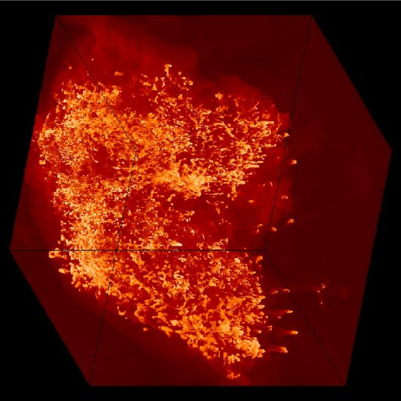
Figure 1: Maximum density values along the lines of sight at one time step of the $1200^{3}$ 2-phase simulation. The brighter spots correspond to a density exceeding 100 cm$-3$ embedded into a pervasive material at a density of a few cm$-3$.

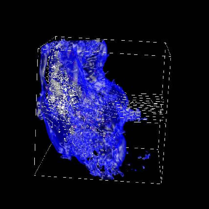
Figure 2: Density isosurface and velocity streamlines at one time step of the 1200³ 2-phase simulation. The large isosurface corresponds to a density of 5 cm^-3 and the white clumps to a density of 500 cm^-3. One can see from the streamlines that the velocity fields is laminar in the WNM and becomes very turbulent in and around the CNM structures.

1 Introduction

Understanding the interstellar turbulence is of great importance in the context of molecular cloud and star formation. As such, many theoretical studies and numerical simulations have been performed during the last decades (see e.g. the reviews by MacLow & Klessen 2004, Scalo & Elmegreen 2004 and Elmegreen & Scalo 2004). So far, most of the studies have considered isothermal flows. Although this constitutes a reasonable assumption for the densest parts of the molecular clouds, it is not an appropriated assumption for the description of the interstellar atomic hydrogen which is 2-phase in nature (e.g., Dickey & Lockman 1990, Field et al. 1969, Wolfire et al. 1995) and therefore for the formation of molecular clouds. Indeed, recent works (Hennebelle & Inutsuka 2006, Vázquez-Semadeni et al. 2007, Heitsch et al. 2008a, Hennebelle et al. 2008, Banerjee et al. 2009) have investigated the possibility that molecular clouds are multi-phase objects. It seems therefore important to understand the dynamical properties of a turbulent 2-phase medium as the interstellar atomic gas.

Various studies have been already performed along this line. This includes 1D calculations (Hennebelle & Pérault 1999, Koyama & Inutsuka 2000, Sánchez-Salcedo et al. 2002, Inoue et al. 2006), 2D calculations (Koyama & Inutsuka 2002, Audit & Hennebelle 2005, Heitsch et al. 2005, 2006) and 3D calculations (Kritsuk & Norman 2002, Gazol et al. 2005, Vázquez-Semadeni et al. 2006). The influence of the magnetic field on the dynamics of a thermally bistable flow has been investigated by Hennebelle & Pérault (2000), Piontek & Ostriker (2004, 2005), de Avillez & Breitschwerdt (2005), Hennebelle & Passot (2006), and more recently by Inoue & Inutsuka (2008), Hennebelle et al. (2009), Heitsch et al. (2009), Inoue et al. (2009) and Gazol et al. (2009).

In a previous study, Hennebelle & Audit 2007, (hereafter HA07) and Hennebelle et al. (2007), we have investigated the dynamics of 2-phase flows by the means of bidimensional high resolution numerical simulations. In particular, we have studied the properties of the dense and cold clumps formed out of the warm gas by thermal instability, showing that they present many similarities with observed clumps. In the present paper, we investigate the properties of clumps formed in more realistic 3D simulations. To better understand the influence of the 2-phase physics and since the nature of the inter-clump gas within molecular clouds is not well known (see §4.1 for a discussion), we also perform isothermal and polytropic simulations having identical setups as the 2-phase ones but for the thermal properties. We then compare the results obtained for the various types of simulations.

The plan of the paper is the following, in the second section we describe the numerical experiments we perform, in the third section we present the global properties of the numerical simulations including the density PDF and the Mach number-density distribution. The fourth section is devoted to the clump properties including their mass spectrum, velocity dispersion and mass-size relation. In the fifth section we summarize our results and conclude the paper.

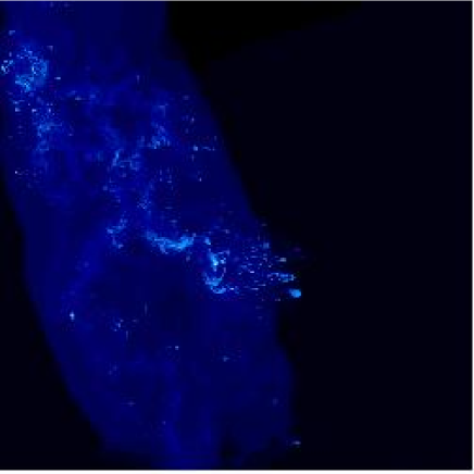
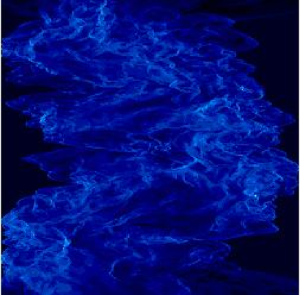
Figure 3: Density cut through the simulations. The left plot corresponds to the 2-phase run and the right one to the isothermal run. Bright regions correspond to a density between 20 cm^-3 and 100 cm^-3 while the pervasive grey area corresponds to a density of a few cm^-3.

2 Initial conditions and method

The equations are identical to those used in our previous studies and can be found in Audit & Hennebelle (2005), (hereafter AH05). However, one difference with the study performed by HA07 is that we do not include thermal conduction in the 3D runs. As emphasized in HA07, it does not have a major effect except on the very small scale structures which due to insufficient numerical resolution, are not any way described in the present simulations.

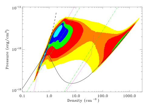
Figure 4: Distribution of mass in the density-pressure plan. The solid line corresponds to the thermal equilibrium curve, the dashed curve corresponds to the Hugoniot curve of shocked gas and the dashed-dotted lines are the isothermal curves at $T=5000$ K and $T=200$ K and the region between the dotted curves is the region where the gas is thermally unstable.

We use the HERACLES code to perform the simulation. This is a second order Godunov type hydrodynamical code. The size of the computational domain is $15$ pc and the resolution ranges from $600^{3}$ to $1200^{3}$ cells leading to a spatial resolution of $2.5\times 10^{-2}$ to $1.25\times 10^{-2}$ pc. Let us remind that in HA07, the highest resolution run had $10\;000^{2}$ cells corresponding to a spatial resolution of $2\times 10^{-3}$ pc. As stated in HA07, the resolution has a strong influence on the results and must be sufficient to cover a large dynamics of spatial scales. Typically, 2500² to 5000² cells were needed to get some reliable numerical convergence even if no strict numerical convergence could be obtained. Therefore, the present runs are likely to be affected by insufficient numerical resolution. However, we stress that it is nowadays difficult to do much bigger runs in 3D than the one we perform. We believe, nevertheless, that investigating the 3D effects is worthwhile even with a relatively low resolution. One should however keep in mind this restriction when looking at the results.

Since our primary goal is to investigate the exact influence of equations of state on the dynamics of the flow, we have done simulations of 2-phase flows (using the cooling function described in AH05) and using an isothermal equation of state with a temperature of 100 K. Finally, since it has been found that the effective polytropic index of the cold gas is about 0.7, we have performed a simulation using a polytropic equation of state with a polytropic index of $\gamma=0.7$. For this run the temperature is given by

$$T=100\,{\rm K}\,({\rho\over 100\,{\rm cm}^{-3}})^{-0.3}.$$ (1)

For all the simulations, the boundary conditions consist in an imposed converging flow (see AH05, Folini & Walder 2006) at the left and right faces of amplitude $V_{in}\simeq$15 km s^-1 (which corresponds to $\simeq 1.5\times C_{s,wnm}$ where $C_{s,wnm}$ is the sound speed of the warm neutral medium) on top of which fluctuations of various amplitudes have been superimposed. We stress that since the mean velocity is the same for all the runs, this implies that while 2-phase simulations are mildly transsonic (this is of course no longer the case for the cold gas produced in these simulations) with Mach number ${\cal M}\simeq 1.5$, the isothermal and barotropic ones are very supersonic with Mach numbers of the order of 10. The initial conditions are also identical to the one used in AH05, that is to say a uniform low density gas of density $n_{\rm in}\simeq 0.8$ cm^-3 which is also the density of the incoming flow for all the runs. In the 2-phase case, this gas is at thermal equilibrium and corresponds to WNM (i.e. has a temperature of about 8000 K).

For the 3 types of simulations, the ram pressure of the incoming flow is thus $n_{\rm in}m_{p}V_{in}^{2}=n_{\rm in}m_{p}\times(1.5\times C_{s,wnm})^{2}\simeq 2.15\times k_{b}n_{\rm in}T_{WNM}\simeq 1.4\times 10^{4}k_{b}$ K cm^-3, where $T_{WNM}$ is the temperature of the WNM which is of the order of 8000 K, $k_{b}$ is the Boltzmann constant and $m_{p}$ the mean molecular weigth. In the 2-phase case, the thermal pressure of the diffuse gas injected inside the box is about $(3/2)k_{b}n_{\rm in}T_{WNM}\simeq 1.2\times 10^{4}k_{b}$ K cm^-3 while it is $(3/2)k_{b}n_{\rm in}\times(100K)\simeq 150k_{b}$ K cm^-3 in the isothermal case. The latter is thus roughly 80 times smaller than the former.

For the four other faces, outflow conditions have been setup, implying that the flow can escape the computational box across these four faces. The advantage of this setup, which consists in focusing on a peculiar large scale events, is clearly the spatial resolution of the CNM structures. In particular, considering a turbulent forcing would require a larger box to produce large scale events at the scale of the WNM cooling length, therefore increasing the size of the computational cells. We stress that this is different from polytropic flows in which there is no cooling length to be considered.

The simulations are then runned until a statistically stationary state is reached. This constitutes a difference with other related work (e.g., Koyama & Inutsuka 2002, Heitsch et al. 2006) which investigate the development of the thermal and dynamical instabilities. In order to reach more rapidly the statistically stationary state, we start with a coarser numerical resolution and we then double it once statistical stationarity has been reached.

In order to study the influence of various physical parameters, and more specifically of the cooling function, we have performed several runs assuming different thermo-dynamical properties for the gas. First of all, we have done three runs with a 2-phase flow using the heating/cooling function presented in AH05. For these three runs, the amplitude of the velocity fluctuations imposed on the boundary was given by $\epsilon=1,2$ and $4$ corresponding to modulations of the order of 10 %, 20 % and 40 % respectively (see AH05 for details). The effect of varying the amplitude of the fluctuations imposed at the boundaries is to increase the turbulence in the box. To quantify this effect, we have computed the mean shear for each value of $\epsilon$. The average shear is computed in the following way: in each cell, we compute the velocity stress tensor (i.e., $\partial_{x_{i}}V_{j}$). We then diagonalize the symmetric trace-free part of this tensor and the shear is defined as the root-mean square of the obtained eigenvalues. We finally compute the average over all cells in the simulation. Table 1 gives the value of the mean shear for $\epsilon=$1, 2 and 4. The isothermal run was done using $\epsilon=2$ for the boundary conditions.

3 Global statistics

3.1 General morphology of the flow

Figure 1 shows the maximum of the density field along the lines of sight at a particular time step, after statistical stationarity has been reached in the box for the 2-phase run in the case $\epsilon=1$. The morphology is rather complex. The cold gas seen in white and yellow is very fragmented and very structured. The warm and diffuse gas appears to be intrusive. This is qualitatively similar to the structure observed in 2D simulations (see AH05 and HA07) although some differences can be seen. For example, the 2D simulations seems to be more filamentary. It is worth, however, to recall at this stage that the resolution is 5 to 10 times smaller in this run than in the highest resolution run presented in HA07.

Figure 2 diplays density isosurfaces and velocity streamlines at the same time step. The large isosurface corresponds to a density of 5 cm^-3 and therefore traces mainly the WNM compressed by the ram pressure of the converging flow. The white clumps corresponds to a density of 500 cm^-3 and therefore mainly shows the dense CNM structures confined by the thermal and the ram pressure of the surrounding WNM. The streamlines show that the velocity field is nearly laminar in the WNM and becomes very turbulent inside the compressed layer and therefore around the CNM structures. This is similar to what is reported by Heitsch et al. (2006, 2008b) who point out the influence of the Kelvin-Helmholtz instability as a plausible source of turbulence within the forming cloud.

Figure 3 displays density maps of a slice of the 2-phase run (left) and of the isothermal one (right). The visual aspect of the density field in these two simulations is quite different. First of all, while the dense isothermal flow tends to be distributed in a large fraction of the box, most of the dense gas in the 2-phase flow is concentrated in a thin layer located at the onset of the 2 converging flows. This is partly due to the thermal pressure which is higher in the 2-phase case than in the isothermal gas and can efficiently push the gas outside the computing box (indeed as discussed later the total mass is higher in the isothermal case than in the 2-phase case). However, we have also performed runs with periodic boundary conditions along the y and z-directions which show the same trends although slightly reduced. Thus, we think that other dynamical processes such as the development of the non linear thin shell instability (Vishniac 1994) is also playing a role here. Indeed, for this instability to develop, the slab must be locally displaced by at least a distance comparable to its thickness. As a consequence, the non linear thin shell instability develops only, or at least is much stronger, when the incoming flows are supersonic. While in the 2-phase case, the flows are transsonic (since the sound speed of the WNM is about 10 km s^-1, they are highly supersonic (${\cal M}\simeq 10$) in the isothermal case.

Second of all, in the 2-phase case, one sees spheroid structures, with some filaments surounded by a more diffuse medium. In the isothermal case, the density structures are largely imprinted by bow shocks and clumps can hardly be seen. As we will see further the density PDF and Mach number distribution are indeed very different in both cases. However, these large differences are not so obvious anymore when looking at the statistics of dense structures.

3.2 Pressure and density distributions

Figures 4 show a bidimensional pressure-density histogram. The solid line is the thermal equilibrium curve, the two dashed-dotted lines correspond to constant temperature ($T=5000$ and 200 K) and the dashed line corresponds to the Hugoniot curve. As in previous studies (Vázquez-Semadeni et al. 2003, AH05), we see that if most of the gas lies near the two branches of equilibrium ($T\simeq 8000$ K for the WNM and $T\simeq 50-100$ K for the CNM), a significant fraction is nevertheless in the thermally unstable domain. As pointed out in AH05, there is a clear correlation between the level of turbulence and the fraction of this thermally unstable gas indicating that turbulence is the main cause for the existence of this gas. This can be seen in table 1, where the fraction of cold and unstable gas is given for each 2-phase runs as well as the mean value of the shear. It is clear that the shear inhibits the formation of cold structures. For the two runs with the lowest value of $\epsilon$ ($\epsilon=1$ and $2$), we find, as in AU05, that the amount of cold and unstable gas is independant of the turbulence but that the formation of cold gas is strongly inhibited by the shear. In other words, the shear does not prevent the formation of thermally unstable gas but does prevent the formation of cold dense gas out of the thermally unstable gas.

For $\epsilon=4$, the shear is so strong that cold structures can hardly form. For this reason, in the following we emphasize the $\epsilon=1$ case which contains a larger fraction of CNM providing better statistics on the dense gas than the other cases. In the appendix the results corresponding to the $\epsilon=2$ case are displayed.

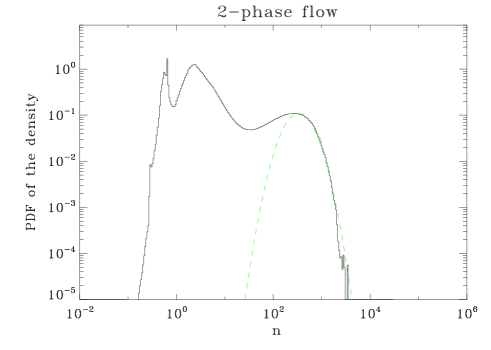
Figure 7: Probability distribution function of the density for the 2-phase run.

The probality distribution function (PDF) of the density for the 2-phase, isothermal and polytropic runs are plotted on Figs. 5, 6 and 7, respectively. The density PDF, $P(n)$, of isothermal simulations has been studied by various authors (e.g. Padaon et al. 1997, Passot & Vázquez-Semadeni 1998) and has been found to be lognormal. More precisely, the following formulae has been proposed:

$$P(n)=\frac{a}{\sqrt{2\pi\sigma^{2}}}\exp(-\frac{(\ln(n)-\ln(\bar{n})-0.5\sigma^{2})}{2\sigma^{2}})$$ (2)

with $\sigma^{2}=\ln(1+b^{2}{\cal M}^{2})$. The fits shown in the figures were obtained using the parameters given in table 2. The dotted line in Fig. 6 corresponds to $n^{-3/2}$.

As found by previous authors, the isothermal PDF is well fitted by this lognormal distribution, eventhough we get slightly larger wings. This may be due to our forcing which is not applied in the Fourier space and in the solenoidal modes as it is the case in most of the compressible simulations which have been performed. Indeed, Federrath et al. (2008) find that while forcing in the compressible modes rather than in the solenoidal ones, large non Gaussian wings develop. Since our forcing is exerted from the boundaries as a converging flow and therefore, at the scale of the box at least, mainly in the compressible modes, it seems likely to us that such an effect is certainly playing a role in our simulation. The value of the $b$ parameter, namely $b=0.33$ is also reminiscent of the values quoted in the literature (e.g. Federrath et al. 2008).

In the $\gamma=0.7$ polytropic case, the low density part of the PDF is well fitted by a lognormal distribution, while for higher density, the PDF is a powerlaw whose exponent is about -1.5. Such powerlaws have been numerically found and explained in Passot & Vázquez-Semadeni (1998) for 1D simulations It is typical of very compressible fluids ($\gamma<1$) and is a direct consequence of the thermal pressure term. Indeed, for $\gamma=0.5$, Passot & Vázquez-Semadeni (1998) report an exponent of about -1.2 which appears to be close to our result. Since the value of the exponent that we inferred here is in good agreement with their estimate, it seems that the 3D effects are not altering their conclusion. Note that the value of the $b$ parameter quoted in table 2 is only indicative since as seen from Fig. 6, the lognormal distribution does not provide a good fit to the high density part of the PDF.

For the 2-phase run, we obviously cannot get a lognormal PDF since by definition, the PDF is bimodal. However, it is nevertheless interesting to investigate to what extend the cold gas can be fitted by a lognormal distribution. Table 2 gives the parameter values. Note that the Mach number has been estimated by selecting computational cells of density larger than 20 cm^-3. As can be seen, the high density part of the cold gas density distribution is reasonably reproduced by a lognormal fit. This is a little surprising to us since the effective polytropic index of the CNM is smaller than 1 and indeed not far from 0.7 as can be seen in Fig. 4. We speculate that the numerical resolution of the CNM structures available in the present simulations, is not sufficient to describe this behaviour. We note however that the low density part of the CNM, ranging from $\simeq 10$ cm^-3 up to the peak at $\simeq$ 300 cm^-3, is not well described by a lognormal distribution. This clearly raises the question of what density PDF should be considered in models of molecular clouds.

Finally, it is worth noting that the mean density, or equivalently the total mass, in the box is different for the 3 types of flows. While for the 2-phase flow, the mean density is about 2 cm^-3, its value is about 3.5 cm^-3 for the barotropic flow and 6 cm^-3 for the isothermal case. This is a natural consequence of the average temperature being larger in the 2-phase case than in the barotropic flow which itself has a larger temperature than the isothermal flow. Indeed, since the temperature in our isothermal run is uniformly low compared to the dynamical pressure, the interclump gas cannot confine significantly the clumps which are therefore re-expanding once the shock that has compressed them, has decayed. For this reason, the density of the interclump gas is larger in the isothermal case than in the 2-phase case.

3.3 Distribution of Mach numbers with density

Figures 8 and 9 show the mass distribution in the density-Mach number plan for the 2-phase and the isothermal flow respectively. The isothermal case is very similar to what has been previously reported by Kritsuk et al. (2007) and Federrath et al. (2009). The Mach number is essentially not correlated with the density, with a possible weak anti-correlation.

The two phases can clearly be seen in Fig. 9 and the Mach number varies with the density as about ${\cal M}\propto\rho^{0.5}$. This appears to be roughly consistent with the idea that the velocity dispersion weakly depends on the density while the temperature is roughly proportional to $1/\rho$. This last relation naturally follows from a nearly isobaric model.

Although the two distributions are significantly different, an interesting question is whether the cold gas itself in the 2-phase run behave, thermally but also dynamically, as isothermal or polytropic gas. As already discussed in the previous section and also evident from Fig. 9, this is obviously not the case for the low density part of the dense gas distribution. The question of whether the dense clumps, have similar properties for both types of flows is investigated in the next section.

Table 1: Fraction of unstable and cold gas as a function of the shear

	Cold	Cold	Mean value of
	+ Unstable gas		the shear (Myrs-1)
$\epsilon=1$	0.570	0.121	12.4
$\epsilon=2$	0.569	0.039	15.0
$\epsilon=4$	0.358	0.002	23.4

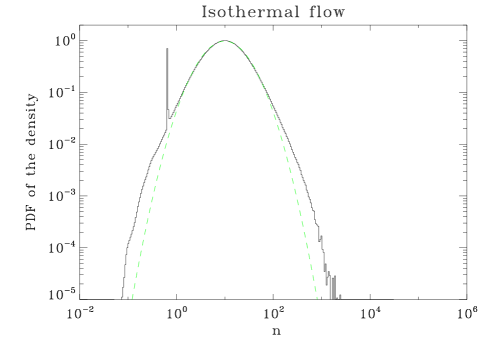
Figure 5: Probability distribution function of the density for the isothermal run. The dashed line is a lognormal fit.

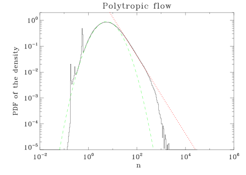
Figure 6: Probability distribution function of the density for the polytropic run. The dashed line is a lognormal fit while the dotted line is a powerlaw fit.

Table 2: Parameters used for the fit of the density pdf

	$\bar{n}$	${\cal M}$	b
2-phase	280	2.48	0.26
Isothermal	6.5	3.49	0.33
polytropic	3.6	2.95	0.4

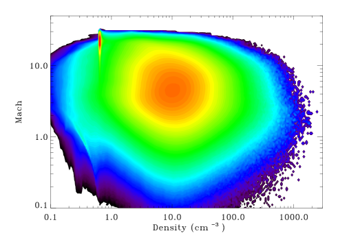
Figure 8: Mass Distribution in the density-Mach number plan for the isothermal flow. The mass excess around $n=0.8$ cm^-3 and ${\cal M}\simeq 15-20$ correspond to the input flow.

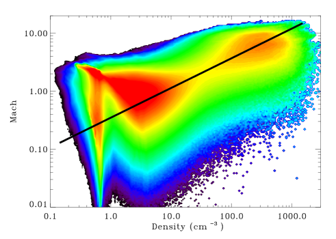
Figure 9: Mass distribution in the density-Mach number plan for the bistable turbulent flow with $\epsilon=1$. The black line corresponds to ${\cal M}\propto\rho^{0.5}$.

4 Properties of CNM structures

In this section, we examine the properties of the dense structures. As in AH05, they are extracted by a simple clipping algorithm using a density threshold, $n_{s}$. In the 2-phase case, 3 values of $n_{s}$ are explored, namely 10, 30 and 100 cm^-3. While the first value lies in the thermally unstable domain, the two others correspond to gas in the cold phase. As for the previous section, we also show corresponding results for isothermal gas. In the isothermal runs however, the value $n_{s}=10$ cm^-3 is too low to allow for structure extraction and therefore only $n_{s}=30$ and 100 cm^-3 are used. This can be clearly seen from Fig. 5 which shows that the density peak is close to 10 cm^-3.

Let us recall that we present the structure properties obtained in the $\epsilon=1$ case for the 2-phase run and $\epsilon=2$ for the isothermal run. The reason is that there are more structures in the $\epsilon=1$ than $\epsilon=2$ case giving better statistics while the distributions are otherwise similar. The corresponding figures for the 2-phase $\epsilon=2$ case are shown in the appendix.

4.1 Relevance of comparison with observations

The question of with which set of data our results should be compared is not entirely straightforward. Strictly speaking, the 2-phase simulations should be compared with HI data such as the one obtained in the Millenium survey (Heiles & Troland 2003). This comparison which was the main purpose of the study performed by Hennebelle et al. (2007), is however restricted. The reason is that the distance of HI clouds is usually unknown because HI is ubiquitous within the Galaxy. Thus, in particular, size and mass spectrum cannot be easily computed. Extragalactic studies such as the one performed by Kim et al. (2007) can get rid of this difficulty, however, the scales that one can probe in nearby galaxies is much larger than the ones tackled in our simulations.

On the other hand, our results are not restricted to 2-phase flows since isothermal and barotropic cases are also considered. These thermal approximations are thought to be fairly reasonable to describe the dense part of molecular clouds (i.e. denser than 10³ cm^-3) and have been used in many studies. Thus it is both interesting and justify to compare the statistics inferred from these numerical simulations with the statistics which have been observationally inferred for molecular clouds.

Finally, the nature of the interclump medium within molecular clouds is still very uncertain. Williams et al. (1995) studied in detail the Rosette molecular cloud and conclude that in this cloud, the interclump medium is a mixture of atomic gas (the density, 2-4 cm^-3, they quote, traditionally corresponds to either warm or thermally unstable HI gas as seen in Fig. 4) and very diffusive H₂. Recent theoretical studies (e.g. Hennebelle et al. 2008, Heitsch et al. 2008, Banerjee et al. 2009) attempting to form molecular gas from the diffusive atomic gas, argue that WNM persists between the clumps inside the molecular clouds. If this assumption is correct, this would imply that molecular clouds are also 2-phase objects, with dense molecular gas embedded into a warm and diffuse atomic phase. For this reason, we believe that with due cautions, comparisons between our 2-phase results and some statistics inferred for molecular clouds are also relevant.

4.2 Clump mass spectrum

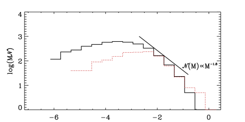
Figure 10: Mass distribution of the structures identified in the 2-phase simulations (A1) with a density threshold $n_{c}=10$ cm^-3. Solid black line shows the 1200³ simulation while red dotted line shows the 600³ simulation. The black straight line shows a clump mass spectrum $dN/dM\propto M^{-1.8}$.

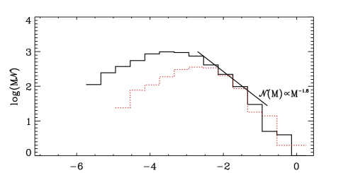
Figure 11: Same as Fig. 10 for a density threshold $n_{c}=30$ cm^-3.

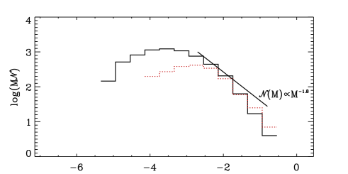
Figure 12: Same as Fig. 10 for a density threshold $n_{c}=100$ cm^-3.

Figure 13: Same as Fig. 10 for the isothermal simulation and a density threshold $n_{c}=30$ cm^-3.

Figures 10-12 show the mass spectrum for the structures extracted from the $600^{3}$ and $1200^{3}$ 2-phase simulations and with a density threshold $n_{s}$ respectively equal to 10, 30 and 100 cm^-3. While the low mass part of the distributions ($<10^{-3}$ solar masses) is spoiled by the numerical resolution, the high mass part ($>0.1$ solar masses) suffer from poor statistics due to the finite size of the box. However, as can be seen by comparing the results of the $600^{3}$ and the $1200^{3}$ simulations, one can see that numerical resolution seems to be nearly reached for intermediate masses. For the three density thresholds, the mass spectrum in this range of masses, approximately follows ${{\cal N}(M)\propto M^{-1.8}}$. It is therefore very similar to what has been inferred in the 2D simulations presented in HA07. It is also similar to the mass spectrum inferred by Dib et al. (2008).

Figure 13 shows the mass spectrum in the isothermal case for $n_{c}=30$ cm^-3. The distribution is rather similar to the 2-phase case except interestingly that more small scale structures are found. We interpret this as being a consequence of the effective (or numerical) Field length preventing the formation of CNM structures of size too close to the mesh. As for the 2-phase case, the mass spectrum between $10^{-3}$ and $10^{-1}$ solar masses, is a powerlaw whose exponent is close to $1.8$.

Let us recalled that in HA07, we propose a theory to explain the mass spectrum of the CNM structures which predicts $\gamma=16/9$ in 3D and is therefore compatible with the numerical results. This theory, which is based on the Press & Schecter (1974) formalism and assume that the structure mass spectrum reflects the density fluctuations arising in the trans-sonic WNM, has been recently extended by Hennebelle & Chabrier (2008) to the supersonic case. In particular, the exponent of the structure mass spectrum is related to the exponent of the powerspectrum of $\log(\rho)$, $n^{\prime}$, through the relation:

$${dN\over dM}\propto M^{-\beta}=M^{-2+{n^{\prime}-3\over 3}}.$$ (3)

In order to verify this relation, we have computed the powerspectrum of $\log(\rho)$. The 2-phase case is presented in Fig. 14 while the isothermal one is shown in Fig. 15. The value of the exponent is measured to be about 3.3 while as in Kritsuk et al. (2007), we identify a bottle neck in which the exponent is slightly shallower. This value of the exponent is similar to what is reported in Schmidt et al. (2009) thought slightly smaller since they infer a value closer to 3.8. We speculate that this maybe due to our boundary conditions since in a significant fraction of the computational box, the flow is not fully turbulent.

Taking $n^{\prime}\simeq 3.3$, we get with Eq.(3), $\beta\simeq 1.9$ which appears to be compatible with the mass spectrum inferred from the simulations. Taking into account the value inferred by Schmidt et al. (2009), i.e. $n^{\prime}=3.8$, we get $\beta\simeq 1.75$. We also note that the theory presented in HA07 and in Hennebelle & Chabrier (2008) predicts that the mass spectrum exponent should not depend on the density threshold which seems to be compatible with the results displayed in Figs. 10-12. Note that with larger values of $n_{c}$, the mass spectrum we get is not sufficiently accurate to obtain reliable estimate of the exponent. Finally, the mass spectra obtained for different values of $\epsilon$, the fluctuation amplitude imposed at the boundaries, are very similar to the mass spectra presented above, as shown in the appendix.

It is remarkable that the mass spectra obtained under different conditions of forcing and for different thermodynamical behaviors are so similar particularly because significant density PDF have been inferred. Indeed, this strongly suggests that turbulence whose behaviour tends to be universal, is mainly responsible of the shape of the mass spectrum as indicated by Eq. (3).

The value of $\beta$ inferred from the simulations are also compatible with the value quoted in various observational studies (e.g. Blitz 1993, Heithausen et al. 1998) for the CO clumps. Interestingly enough, the structure masses in the sample of Heithausen et al. (1998) are as small as one Jupiter mass and therefore compatible with the mass of the structures formed in our simulations. Although straightforward comparison and therefore conclusion should be taken with care at this stage, since the present work focuses on HI and does not treat neither the formation of H₂ nor the formation of the CO molecule, the universality of the mass spectrum that we observed in our simulations suggests that these processes likely do not affect the mass spectrum significantly. We also note that in a recent study, Kim et al. (2007) inferred similar values for the HI clouds in the small magellanic cloud. The mass of these clouds (10^4-6 solar masses) is however much larger than the mass of our simulated clouds.

Figure 14: Compensated power spectrum $P_{k}k^{n^{\prime}}$ of the logarithm of the density with $n^{\prime}=3.3$ for the weakly turbulent simulation. The two dashed horizontal lines correspond to slopes of -3.3 and -3.1.

Figure 15: Compensated power spectrum $P_{k}k^{n^{\prime}}$ of the logarithm of the density with $n^{\prime}=3.3$ for the isothermal simulation. The two dashed horizontal lines correspond to slopes of -3.3 and -3.1.

4.3 Clump mass size relation

In this section, we investigate the mass-size relation. As in HA07, the size is defined by computing the inertia matrix and taking its largest eigenvalue. Note that we have tried other choices, like for example the geometric means of the 3 eigenvalues and it does not change the results significantly.

Figure 16: Mass versus size relation for the CNM structures extracted from the 2-phase $1200^{3}$ cells simulations.

Figure 17: Mass versus size relation for the structures extracted from the isothermal $1200^{3}$ cells simulations.

Figure 16 shows the mass versus size relation for the CNM structures extracted from the $1200^{3}$ cells simulations for a value of $n_{c}$=30 cm^-3. Structures obtained with $n_{c}=$ 10 and 100 cm^-3 show very similar behaviors and are therefore not displayed here for conciseness. This is also the case for the structures formed in simulations with a larger fluctuation amplitude, $\epsilon=2$ as can be seen in the appendix. The straight line represents a linear fit of the whole distribution. The slope is about 2.2. As can be seen, it represents well the distribution over the whole range of masses.

Figure 17 shows the mass versus size relation for the structures of the isothermal simulation. The slope is about 2.25 and therefore very similar to the 2-phase case. The shape of the distribution is slightly different from the 2-phase case and tends to be closer to a straight line. The similar behaviour obtained for isothermal and 2-phase flows, again suggests that turbulence is the main mechanism responsible of the structure’s shape. The slope of 2.25 derived from our simulation, is very close to what is reported in Kritsuk et al. (2007) and Federrath et al. (2009) although they use different definitions and algorithms than ours which is more appropriate to compare with observations.

Finally, it is worthwhile to recall that the value of 2.3 has been obtained by Heithausen et al. (1998) and Kramer et al. (1998) for the CO molecular clumps. Using a larger sample of data, Falgarone et al. (2004) also conclude that $M\propto L^{2.3}$ is more compatible with the data than the relation $M\propto L^{2}$, originally quoted by Larson (1981).

4.4 Velocity dispersion within structures

Figure 18: Velocity dispersion versus size relation of the CNM structures extracted from the 2-phase $1200^{3}$ cells simulations for $n_{c}=10$ cm^-3.

Figure 19: Same as Fig. 18 for $n_{c}=30$ cm^-3.

Figure 20: Same as Fig. 18 for $n_{c}=100$ cm^-3.

Figure 21: Velocity dispersion versus size relation of the structures extracted from the $1200^{3}$ cells isothermal simulations for $n_{c}=30$ cm^-3.

Figure 22: Velocity dispersion versus size relation of the structures extracted from the $1200^{3}$ cells isothermal simulations for $n_{c}=100$ cm^-3.

Figures 18-20 show the total internal velocity dispersion versus size for the CNM structures, i.e. $\sqrt{\delta V_{x}^{2}+\delta V_{y}^{2}+\delta V_{z}^{2}}$ as a function of $L$ for $n_{c}$ equal to respectively 10, 30 and 100 cm^-3 in the 2-phase case, where $\delta V$ is the velocity with respect to the structure mean velocity. The straight line represents a linear fit of the distribution. While the relation $\sigma\simeq 3.3$ km s^-1 ($L$/1 pc)^0.53 is inferred for $n_{c}$=10 cm^-3, we find $\sigma\propto 2$ km s^-1 ($L$/1 pc)^0.43 for $n_{c}$=30 cm^-3 and $\sigma\propto 1.2$ km s^-1 ($L$/1 pc)^0.33 for $n_{c}$=100 cm^-3. It is interesting to note that for the three values of $n_{c}$, $n_{c}\sigma^{2}(L)$ is roughly the same. That is 10$\times$3.3${}^{2}\simeq 30\times 2^{2}\simeq 100\times 1.2^{2}$. This suggests that kinetic energy tends to be equally distributed in the volume rather than in the mass of the flow. Moreover, it is also interesting to note that this dynamical or turbulent pressure is of the same orders as the thermal pressure and incoming ram pressure. Indeed, for $n_{c}$=100 cm^-3 the thermal pressure of the clump is about $10^{4}k_{b}$ K cm^-3 since the temperature is about 50K-100K while the turbulent pressure is about $2\times 10^{4}k_{b}(L/1pc)^{2}$ K cm^-3, as calculated previously the ram pressure of the incoming flow is about $2\times 10^{4}k_{b}$ K cm^-3. Note that in the velocity dispersion, all the motions have been counted irrespectively of the fact that their could be solenoidal, converging or diverging modes. Straighforward interpretation of this velocity dispersion as a turbulent pressure is therefore not entirely obvious and certainly not accurate within more than a factor of a few.

Figures 21-22 show the total velocity dispersion versus size for $n_{c}$ equal to respectively 30 and 100 cm^-3 in the isothermal case. In both cases, we find a similar relation of about $\sigma\simeq 5$ km s^-1 ($L$/1 pc)^0.55 although for $n_{c}=100$ cm^-3, there are no clump of size bigger than 0.5 pc and very few with size bigger than 0.3 pc. Interestingly, this is a different behaviour than for the 2-phase case since the energy is now more concentrated in dense regions.

These results suggest that 2-phase and isothermal flows behave somehow differently. In particular, since the velocity dispersion is about 2 to 3 times higher while the forcing is identical in both cases, energy is more efficiently injected into the dense clumps in isothermal flows than it is in 2-phase flows. Three, not exclusive, interpretations sound possible to us. First, in the 2-phase flow, energy is efficiently radiated away, in particular during the transition between the warm and the cold phase, where the effective adiabatic exponent is negative. Second, in the 2-phase flows, the clumps are long living since they are bounded by the external pressure. Thus, after a crossing time most of the turbulent motions, initially present in the structure have dissipated. This is different from the isothermal case in which the structures do not survive more than an expansion time since they are not confined by the external thermal pressure. Third, since the dense structures possess sharp edges in the 2-phase flow while in the isothermal one, the transition between dense and rarefied gas is continuous, the coupling between the dense material and the external medium is weaker for the former than for the latter. In particular, it sounds likely that sound waves should be more efficiently reflected by the stiff discontinuities in the 2-phase case. Making a quantitative estimate of these effects is difficult at this stage.

The value of the exponent 0.3-0.5 in this relation is again remarkably similar to what is inferred observationally in our galaxy (e.g., Larson 1981). It is also in good agreement with the index of the velocity powerlaw, $P(v)$, being in the range 11/3 to 4 as inferred from many numerical simulations (e.g., Kritsuk et al. 2007). Let us recall that if $\sigma\propto L^{\eta}$ and $P(v)\propto k^{-\alpha}$, then $\alpha-3=2\eta$.

We note however, that while the slope of the velocity-size relation is approximately correct, its value itself may be too high. Indeed one infers from observations of the CO clumps, the value 1 km s^-1 for the line width which corresponds to about 0.4 km s^-1 for the velocity dispersion along the line of sight and therefore to about $\simeq$0.8 km s^-1 for the total velocity dispersion assuming isotropy which is smaller than what we infer here by a factor 1.5 to 3 in the 2-phase case and about 5-6 in the isothermal one. Note that since the density of the CO clumps is of the order of 3000 cm^-3, the comparison cannot be more than indicative at this stage. We also note that the velocity dispersion decreases with increasing density in our 2-phase simulations suggesting that the velocity dispersion could be very similar to what has been inferred by Larson (1981) for denser clumps. Since the velocity dispersion, directly depends on the forcing, another possibility is that the forcing is a little too strong and should be reduced to better fit the mean ISM conditions.

5 Conclusion

In this paper, we perform 3D high resolution numerical simulations of converging flows using either a standard interstellar atomic cooling function, an isothermal or a polytropic equation of state with an adiabatic index of $\gamma=0.7$.

We investigate the density PDF and Mach number-density relation, showing that, as expected, the thermal behaviour of the gas has a drastic influence. While as previous authors, we find that the isothermal runs tend to produce lognormal density distributions, when the adiabatic exponent is smaller than one, namely $\gamma=0.7$, we find that the density distribution follow a powerlaw for high densities confirming the result of Passot & Vázquez-Semadeni (1998). The 2-phase case is very different thought the high density part of the distribution could reasonably be described by a lognormal distribution. We stress that higher numerical resolution may well change this conclusion. However, the distribution of the low density (say in the range 10-300 cm^-3) cold gas departs significantly from it, making unclear the use of the lognormal density distribution an adequate choice for molecular clouds.

We compute the mass spectrum of the clumps for various density thresholds, as well as the mass-size relation and the internal velocity dispersion-size relation. We find that the 3 distributions agree with the statistics inferred for the interstellar clouds (e.g. Heithausen et al. 1998) reasonably well. In particular, the 3 distributions are well fitted by a powerlaw whose exponent values are close to the observed ones. While the first 2 appear to be reasonably similar for isothermal and 2-phase flows, we find that the internal velocity dispersion is about 2 to 3 times larger for the clumps of the isothermal simulation than for the ones of the 2-phase case, suggesting that energy is less efficiently injected into the dense clumps in 2-phase flows than it is in isothermal ones.

Altogether, these results confirm the claim made in HA07 that 2-phase flows behave differently than isothermal flows. Although it appears to us that higher resolution simulations should be performed to further assess this conclusion, the present study suggests that the 2-phase nature of the flow may have significant implications even for the physics of high density gas.

6 Acknowledgments

We thank Christoph Federrath for a critical reading of the manuscript as well as an anonymous referee for his/her help in clarifying the original version of this work significantly. This work was granted access to the HPC resources of CCRT and CINES under the allocation x2009042204 and x2009042036 made by GENCI (Grand Equipement National de Calcul Intensif). EA acknowledge support from the French ANR through the SiNERGHy project, ANR-06-CIS6-009-01.

Appendix A Statistics for clumps in the $\epsilon=2$ simulation

Here, for completeness, we give the various statistics of the clumps formed in the simulation performed with $\epsilon=2$.

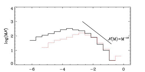
Figure 23: Mass distribution of the structures identified in the 2-phase simulations (A2) with a density threshold $n_{c}=10$ cm^-3. Solid black line shows the 1200³ simulation while red dotted line shows the 600³ simulation. The black straight line shows a clump mass spectrum $dN/dM\propto M^{-1.8}$.

Figure 24: Same as Fig. 23 for a density threshold $n_{c}=30$ cm^-3.

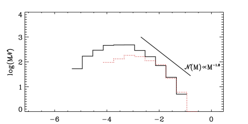
Figure 25: Same as Fig. 23 for a density threshold $n_{c}=100$ cm^-3.

Figure 26: Mass versus size relation for the CNM structures extracted from the $1200^{3}$ cells simulations with $\epsilon=2$ for $n_{c}=10$.

Figure 27: Same as Fig. 26 for $n_{c}=30$ cm^-3.

Figure 28: Same as Fig. 26 for $n_{c}=100$ cm^-3.

Figure 29: Velocity dispersion versus size relation of the CNM structures extracted from the 2-phase $1200^{3}$ cells simulations for $n_{c}=10$ cm^-3.

Figure 30: Same as Fig. 29 for $n_{c}=30$ cm^-3.

Figure 31: Same as Fig. 29 for $n_{c}=100$ cm^-3.

References

- (1) Audit, E., & Hennebelle, P. 2005, A&A 433, 1
- (2) de Avillez, M., & Breitschwerdt, D. 2005, A&A 436, 585
- (3) Banerjee, R., Vázquez-Semadeni, E., Hennebelle, P., Klessen, R., 2009, MNRAS, 398, 1082
- (4) Blitz, L., 1993, prpl.conf, 125
- dib (2008) Dib, S., Brandenburg, A., Kim, J., Gopinathan, M., André, P., 2008, ApJ, 678L, 105
- (6) Dickey, J., & Lockman, F. 1990, ARA&A, 28, 215
- (7) Elmegreen, B., Scalo, J., 2004, ARA&A, 42, 211
- (8) Falgarone, E.; Hily-Blant, P.; Levrier, F.; 2004, Ap&SS, 292, 285
- (9) Federrath, C., Klessen, R., Schmidt, W., 2008, ApJ, 688L, 79
- (10) Federrath, C., Klessen, R., Schmidt, W., 2009, ApJ, 692, 364
- (11) Federrath, C., Duval, J., Klessen, R., Schmidt, W., Mac Low, M.-M., 2009, A&A, submitted, arXiv0905.1060
- (12) Field, G., Goldsmith, D., & Habing, H. 1969, ApJ Lett 155, 149
- (13) Folini, D., & Walder, R. 2006, A&A, 459, 1
- (14) Gazol, A., Luis, L., Kim, J., 2009, ApJ 693, 656
- (15) Gazol, A., Vázquez-Semadeni, E., & Kim, J. 2005, ApJ 630, 911
- (16) Heiles, C., & Troland, T. 2003, ApJ 586, 1067
- (17) Heithausen, A., Bensch, F., Stutzki, J., Falgarone, F., & Panis, J.-F. 1998, A&A 331, L65
- (18) Heitsch, F., Burkert, A., Hartmann, L., Slyz, A., Devriendt, J. 2005, ApJ 633, 113
- (19) Heitsch, F., Slyz, A., Devriendt, J., Hartmann, L., Burkert, A. 2006, ApJ 648, 1052
- (20) Heitsch, F., Hartmann, L., Slyz, A., Devriendt, J., Burkert, A. 2008, ApJ 674, 316
- (21) Heitsch, F., Hartmann, L., Burkert, A. 2008, ApJ 683, 786
- (22) Heitsch, F., Stone, J., Hartmann, L., 2009, ApJ, 695, 248
- (23) Hennebelle, P., & Audit, E. 2007, A&A, 465, 431
- (24) Hennebelle, P., Audit, E., & Miville-Deschènes, M.-A. 2007, A&A, 465, 445
- (25) Hennebelle, P., & Pérault, M. 1999, A&A 351, 309
- (26) Hennebelle, P., & Pérault, M. 2000, A&A 359, 1124
- (27) Hennebelle, P., & Passot, T. 2006, A&A 448, 1083
- (28) Hennebelle, P., Inutsuka, S.-I. 2006, ApJ, 647, 404
- (29) Hennebelle, P., Chabrier, G., 2008, ApJ, 684, 395
- (30) Hennebelle, P., Banerjee, R., Vázquez-Semadeni, E., Klessen, R., Audit, E., 2008, A&A, 486L, 43
- (31) Inoue, T., Inutsuka, S.-i., & Koyama, H. 2006, ApJ, 652, 1331
- (32) Inoue, T., Inutsuka, S.-i., 2008, ApJ, 687, 303
- (33) Inoue, T., Yamazaki, R., Inutsuka, S.-i., 2009, ApJ, 695, 825
- (34) Kim, S.; Rosolowsky, E.; Lee, Y.; et al. 2007, ApJS, 171, 419
- (35) Koyama, H., & Inutsuka, S. 2000, ApJ 532, 980
- (36) Koyama, H., & Inutsuka, S. 2002, ApJ 564, L97
- (37) Kramer, C., Stutzki, J., Rohrig, R., & Corneliussen, U. 1998, A&A 329, 249
- (38) Kritsuk, A. G., & Norman, M. L. 2002, ApJ 569, L127
- (39) Kritsuk, A. G., Norman, M. L., Padoan, P., & Wagner, R. 2007, ApJ, 665, 416
- (40) Larson, R., 1981, MNRAS, 194, 809
- (41) Mac Low, M.-M., & Klessen, R. S. 2004, Rev. Mod. Phys., 76, 125
- (42) Padoan, P., Nordlund, Å., Bernard, J., 1997, ApJ, 288, 145
- (43) Passot, T., Vázquez-Semadeni, E., 1998, Phys. Rev. E., 58, 4501
- (44) Piontek, R., Ostriker, E., 2004, ApJ, 601, 905
- (45) Piontek, R., Ostriker, E., 2005, ApJ, 629, 849
- Press & Schechter (1974) Press, W., Schechter, P., 1974, ApJ, 187, 425
- (47) Sánchez-Salcedo, F. J., Vázquez-Semadeni, E., & Gazol, A. 2002, ApJ 577, 768
- (48) Schmidt, W., Federrath, C., Hupp, M., Kern, S., Niemeyer, J., 2009, A&A, 494, 127
- (49) Scalo, J., Elmegreen, B., 2004, ARA&A, 42, 275
- (50) Vázquez-Semadeni, E., Gazol, A., Passot, T., & Sánchez-Salcedo, F.J. 2003, in Turbulence and Magnetic Fields in Astrophysics, eds. E. Falgarone & T. Passot (Dordrecht: Springer)
- (51) Vázquez-Semadeni, E., Gómez, G. C., Jappsen, A. K., Ballesteros-Paredes, J., González, R. F., & Klessen, R. S. 2007, ApJ, 657, 870
- (52) Vázquez-Semadeni, E., Ryu, D., Passot, T., González, R., & Gazol, A. 2006, ApJ, 643, 245
- (53) Vishniac, E. T. 1994, ApJ, 428, 186
- (54) Williams, J., Blitz, L., & Stark, A. 1995, ApJ, 451, 252
- (55) Wolfire, M.G., Hollenbach, D., & McKee, C.F. 1995, ApJ, 443, 152