Generalised dimensions of measures on almost self-affine sets

Abstract

We establish a generic formula for the generalised $q$-dimensions of measures supported by almost self-affine sets, for all $q>1$. These $q$-dimensions may exhibit phase transitions as $q$ varies. We first consider general measures and then specialise to Bernoulli and Gibbs measures. Our method involves estimating expectations of moment expressions in terms of ‘multienergy’ integrals which we then bound using induction on families of trees.

AMS classification scheme numbers: 28A80, 37C45

1 Introduction

Let $S_{1},\ldots,S_{m}:{\mathbb{R}}^{N}\rightarrow{\mathbb{R}}^{N}$ be a family of contractions; thus there are constants $c_{i}<1$ such that $|S_{i}(x)-S_{i}(y)|\leq c_{i}|x-y|$ for all $x,y\in{\mathbb{R}}^{N}$. Such a family is known as an iterated function system (IFS), and it is well-known that there exists a unique non-empty compact set $E$ satisfying

$$E=\bigcup_{i=1}^{m}S_{i}(E),$$

called the attractor of the system. If the $S_{i}=T_{i}+a_{i}\,(1=1,\ldots,m)$ are affine contractions, where $T_{1},\ldots,T_{m}$ are non-singular contracting linear mappings on ${\mathbb{R}}^{N}$ and $a_{1},\ldots,a_{m}\in{\mathbb{R}}^{N}$ are translation vectors, we call $E$ a self-affine set, see [10].

The Hausdorff and box-counting dimensions of many self-affine sets $E$ are given by $\min\{d(T_{1},\ldots,T_{m}),N\}$, where

$$d(T_{1},\ldots,T_{m})=\inf\Big{\{}s:\sum_{k=1}^{\infty}\sum_{{\bf i}\in I_{k}}\phi^{s}({T_{{\bf i}}})<\infty\Big{\}},$$

a number sometimes called the affinity dimension of $E$, which is defined in terms of the singular values of iterated compositions of the mappings $T_{i}$, see Section 2 for details. This was shown in [5] to hold for almost all $(a_{1},\ldots,a_{m})\in{\mathbb{R}}^{mN}$ provided that $\|T_{i}\|<\frac{1}{3}$ for all $i$, a restriction that was soon weakened to $\|T_{i}\|<\frac{1}{2}$ in [24]. The affinity dimension turns out to give the Hausdorff or box dimensions of self-affine sets in many other cases, see for example [6, 13, 17], and is regarded as a ‘generic’ formula for the dimensions of self-affine sets. Nevertheless, the dimensions of self-affine sets need not vary continuously with the parameters $(a_{1},\ldots,a_{m})$ and for highly regular constructions such as self-affine carpets (where the $S_{i}$ map a square onto rectangles selected from a rectangular grid) the dimension of the self-affine set is in general strictly less than than its affinity dimension, see [3, 20]. For more on the dimensions of self-affine sets, see the surveys [4, 22].

Recently, Jordan, Pollicott and Simon [15] introduced a variant of self-affine sets, which we will term almost self-affine sets, with rather more randomness allowed in the translation parameters than for strictly self-affine sets. Here an independent random perturbation is made at each stage of the iterated construction of the set, yielding a ‘statistically self-affine’ set, and this was shown to have Hausdorff and box dimensions $\min\{d(T_{1},\ldots,T_{m}),N\}$ almost surely, with the only restriction that $\|T_{i}\|<1$ for all $i$; see (2.8) below. (Note that it is often convenient to use the language of probability rather than of measure theory when considering such constructions.)

It is natural to consider multifractal analogues of these dimension formulae, in particular to seek the generalised $q$-dimensions (also termed generalised Rényi dimensions) of measures supported by self-affine sets. The generalised $q$-dimension of a measure $\tau$ reflects the behaviour of moment sums of $\tau$ over small boxes; it is given for $q>0,q\neq 1$ by

$$D_{q}(\tau)=\lim_{r\rightarrow 0}\frac{\log M_{r}(q)}{(q-1)\log r}$$

provided the limit exists (or taking lower and upper values otherwise), where $M_{r}(q)=\sum_{C\in{\cal M}_{r}}\tau(C)^{q}$, with the sum over the set ${\cal M}_{r}$ of mesh cubes of side $r$, see Section 3 for more details.

There is a natural analogue of the affinity dimension that is appropriate for $q$-dimensions of measures supported by self-affine sets, namely (for $q>1$)

$$d_{q}^{-}(T_{1},\ldots,T_{m};\mu)=\sup\{s:\sum_{k=0}^{\infty}\sum_{{\bf i}\in I_{k}}\phi^{s}({T_{{\bf i}}})^{1-q}\mu(C_{{\bf i}})^{q}<\infty\},$$ (1.1)

where $\mu$ is a measure on the underlying code space (for $0<q<1$ the supremum is replaced by an infimum). One might hope that the (lower) generalised dimensions of self-affine measures would equal $\min\{d_{q}^{-},N\}$ in a ‘generic’ sense. Again, examples such as measures on self-affine carpets show that this cannot be true for all constructions, see [1, 16, 21]. Nevertheless, we showed in [9] that $\min\{d_{q}^{-},N\}$ gives an upper bound if $q>0$, and in the case of $1<q\leq 2$ equals the generalised dimension for almost all sets of translation vectors $(a_{1},\ldots,a_{m})\in{\mathbb{R}}^{mN}$, provided that $\|T_{i}\|<\frac{1}{2}$ for all $i$.

To estimate higher moments, that is to find $D_{q}$ for $q>2$, more randomness seems to be needed, and a very natural setting is for measures supported by almost self-affine sets. Our main result, Theorem 8.1, is that the (lower) generalised $q$-dimension of a measure on an almost self-affine set equals $\min\{d_{q}^{-},N\}$ almost surely for all $q>1$. We first consider general measures on almost self-affine sets, and then specialise to Bernoulli measures and Gibbs measures in Corollaries 8.3 and 8.5 As with self-affine measures for $1<q\leq 2$, see [9], the generalised $q$-dimensions can exhibit phase transitions, corresponding to the non-differentiability of $d_{q}^{-}$ at those $q$ where where $d_{q}^{-}$ is an integer.

Upper bounds for the $q$-dimensions follow from routine methods. Obtaining almost sure lower bounds for the $q$-dimensions is much more involved and breaks into two stages. First, in Section 6, we show that the expectation of (an equivalent integral version of) $M_{r}(q)$ is controlled by certain ‘multienegy integrals’ of the form

$$\int\cdots\int\phi^{s}({\bf i}_{1},\ldots,{\bf i}_{q})^{-1}d\mu({\bf i}_{1})\ldots d\mu({\bf i}_{q})$$

(in the special case where q is an integer) where $\phi^{s}({\bf i}_{1},\ldots,{\bf i}_{q})$ is given in terms of products of singular value functions of iterated products of the $T_{i}$. Then in Section 7 we bound these integrals by breaking up the domain of integration and estimating the integral over each such subdomain using induction on families of trees. This leads to the desired almost sure lower bounds for the $q$-dimensions in Section 8.

2 Definitions and notation

We will work throughout with contracting, non-singular, linear mappings $T\in{\cal L}({\mathbb{R}}^{N},{\mathbb{R}}^{N})$; of course products of such mappings will also be contracting and non-singular. Recall that the singular values $\alpha_{i}\equiv\alpha_{i}(T)$ of $T\;(i=1,\ldots,N)$ are the positive square roots of the eigenvalues of $TT^{\ast}$, where $T^{\ast}$ is the transpose of $T$, or equivalently are the lengths of the (mutually perpendicular) principal semiaxes of $T(B)$, where $B$ is the unit ball in ${\mathbb{R}}^{N}$. We adopt the convention that $1>\alpha_{1}\geq\alpha_{2}\geq\ldots\geq\alpha_{N}>0$. The singular value function $\phi^{s}(T)$ is central in the analysis of self-affine sets. For $0\leq s\leq N$ we define

$$\phi^{s}(T)=\alpha_{1}\alpha_{2}\ldots\alpha_{j-1}\alpha_{j}^{s-j+1},$$

where $j$ is the integer such that $j-1<s\leq j$. It is convenient to set $\phi^{s}(T)=(\alpha_{1}\alpha_{2}\ldots\alpha_{N})^{s/N}=(\det T)^{s/N}$ for $s>N$.

Clearly $\phi^{s}({T})$ is continuous and strictly decreasing in $s$, and is sub-multiplicative, that is, for all $s\geq 0$,

$$\phi^{s}({TU})\leq\phi^{s}({T})\phi^{s}({U})$$ (2.1)

for all $T,U\in{\cal L}({\mathbb{R}}^{N},{\mathbb{R}}^{N})$, see [5] for these basic properties.

Many fractals, including self-similar, self-affine and almost self-affine sets may be constructed in a hierarchical manner which can conveniently be indexed by a code space or sequence space. For $k=0,1,2,\ldots$ let $I_{k}$ be the set of all $k$-term sequences or words formed from the integers $1,2,\ldots,m$, that is $I_{k}=\{(i_{1},i_{2},\ldots,i_{k}):\,1\leq i_{j}\leq m\}$; we take $I_{0}$ to contain just the empty word $\emptyset$. We often abbreviate a word in $I_{k}$ by ${\bf i}=(i_{1},i_{2},\ldots,i_{k})$ and write $|{\bf i}|=k$ for the length of ${\bf i}$. We write $I=\cup^{\infty}_{k=0}I_{k}$ for the set of all such finite words, and $I_{\infty}$ for the corresponding set of infinite words, so $I_{\infty}=\{(i_{1},i_{2},\ldots):1\leq i_{j}\leq m\}$. Juxtaposition of ${\bf i}$ and ${\bf j}$ is written ${\bf ij}$. We write ${\bf i}|_{k}=(i_{1},\ldots,i_{k})$ for the curtailment after $k$ terms of ${\bf i}=(i_{1},i_{2},\ldots)\in I_{\infty}$, or of ${\bf i}=(i_{1},\ldots,i_{k^{\prime}})\in I$ if $k\leq k^{\prime}$. We write ${\bf i}\preceq{\bf j}$ to mean that ${\bf i}$ is a curtailment of ${\bf j}$. If ${\bf i,j}\in I_{\infty}$ then ${\bf i}\wedge{\bf j}$ is the maximal sequence such that both ${\bf i}\wedge{\bf j}\preceq{\bf i}$ and ${\bf i}\wedge{\bf j}\preceq{\bf j}$.

We may topologise $I_{\infty}$ in a natural way by the metric $d({\bf i},{\bf j})=2^{-|{\bf i}\wedge{\bf j}|}$ for distinct ${\bf i},{\bf j}\in I_{\infty}$ which makes $I_{\infty}$ into a compact metric space. The cylinders $C_{\bf i}=\{{\bf j}\in I_{\infty}:{\bf i}\preceq{\bf j}\}$ for ${\bf i}\in I$ form a base of open and closed neighbourhoods of $I_{\infty}$.

It is convenient to identify $I$ with the vertices of an $m$-ary rooted tree with root $\emptyset$. The edges of this tree join each vertex ${\bf i}\in I$ to its $m$ ‘children’ ${\bf i}_{1},\ldots,{\bf i}_{m}$. The estimates in Section 7 involve certain automorphisms of this tree.

Compositions of the contractions $T_{1},\ldots,T_{m}$ will be written $T_{\bf i}\equiv T_{i_{1}}T_{i_{2}}\ldots T_{i_{k}}$ where ${\bf i}=(i_{1},i_{2},\ldots,i_{k})$, with $T_{\emptyset}$ the identity mapping. Set

$$a_{-} = \min_{1\leq i\leq m}\alpha_{n}(T_{i})$$ (2.2)

$$a_{+} = \max_{1\leq i\leq m}\alpha_{1}(T_{i})$$ (2.3)

where $\alpha_{j}(T_{i})$ are the singular values of $T_{i}$. Then $0<a_{-}\leq a_{+}<1$, and

$$a_{-}^{|{\bf i}|}\leq\alpha_{j}(T_{{\bf i}})\leq a_{+}^{|{\bf i}|}$$

for all ${\bf i}\in I$ and $j=1,\ldots,n$, so that

$$a_{-}^{s|{\bf i}|}\leq\phi^{s}({T_{{\bf i}}})\leq a_{+}^{s|{\bf i}|}.$$ (2.4)

We also note that, for $h>0$,

$$a_{-}^{h|{\bf i}|}\phi^{s}({T_{{\bf i}}})\leq\phi^{s+h}(T_{{\bf i}})\leq a_{+}^{h|{\bf i}|}\phi^{s}({T_{{\bf i}}}).$$ (2.5)

We now introduce a notation that will permit a random perturbation at each stage of the hierarchical construction of the attractor as in [15]. Let $D$ be a bounded region of ${\mathbb{R}}^{N}$ and for each ${\bf i}\in I$ let $\omega_{{\bf i}}\equiv\omega_{i_{1},\ldots,i_{k}}\in D$ be a ‘displacement’ or ‘perturbation’ which will eventually be random. Let $\omega=\{\omega_{\bf i}:{\bf i}\in I\}$ denote the aggregate of the $\omega_{{\bf i}}$. Define the projection $\Pi^{\omega}:I_{\infty}\to{\mathbb{R}}^{N}$ by

$$\Pi^{\omega}({\bf i}) = \lim_{k\to\infty}(T_{i_{1}}+\omega_{i_{1}})(T_{i_{2}}+\omega_{i_{1},i_{2}})\cdots(T_{i_{k}}+\omega_{i_{1},\ldots,i_{k}})(x)$$ (2.6)

$$= \omega_{i_{1}}+T_{i_{1}}\omega_{i_{1},i_{2}}+T_{i_{1}}T_{i_{2}}\omega_{i_{1},i_{2},i_{3}}+\cdots.$$ (2.7)

It is easily checked that this limit exists and is independent of $x\in{\mathbb{R}}^{N}$, and that the map ${\bf i}\mapsto\Pi^{\omega}({\bf i})$ is continuous.

We term the compact set

$$E^{\omega}=\bigcup_{{\bf i}\in I_{\infty}}\Pi^{\omega}({\bf i})\subseteq{\mathbb{R}}^{N},$$ (2.8)

an almost self-affine set. Note that if $B\subseteq{\mathbb{R}}^{N}$ is a ball large enough so that $T_{i_{1}}(B)+\omega_{i_{1},\dots,i_{k}}\subseteq B$ for all $i_{1},\dots,i_{k}$ then

$$E^{\omega}=\bigcap_{k=0}^{\infty}\bigcup_{i_{1},\dots,i_{k}\in I_{k}}(T_{i_{1}}+\omega_{i_{1}})(T_{i_{2}}+\omega_{i_{1},i_{2}})\cdots(T_{i_{k}}+\omega_{i_{1},\ldots,i_{k}})(B),$$ (2.9)

which represents the standard hierachical way of constructing $E^{\omega}$.

A standard covering argument, involving dividing up each of the sets in (2.9) into appropriate pieces, shows that for all $\omega$, the Hausdorff and lower and upper box-counting dimensions satisfy

$$\mbox{\rm dim}_{\rm H}\,(E^{\omega})\leq\underline{\mbox{\rm dim}}_{\rm B}\,(E^{\omega})\leq\overline{\mbox{\rm dim}}_{\rm B}\,(E^{\omega})\leq\min\{d(T_{1},\ldots,T_{m}),N\},$$ (2.10)

where

$$d(T_{1},\ldots,T_{m})=\inf\Big{\{}s:\sum_{k=1}^{\infty}\sum_{{\bf i}\in I_{k}}\phi^{s}({T_{{\bf i}}})<\infty\Big{\}};$$ (2.11)

see [5, 15].

There are many situations where equality holds in (2.10). These include self-affine sets (where $\omega_{i_{1},\ldots,i_{k}}=\omega_{i_{1}}$ depends only on the first subscript) for ${\cal L}^{mN}$-almost all $\omega_{i_{1}},\ldots,\omega_{i_{m}}$, provided $\|T_{i}\|<\frac{1}{2}$ for all $i$, see [5, 24]. Equality also holds with probability one for the almost self-affine sets introduced in [15], where the $\{\omega_{\bf i}:{\bf i}\in I\}$ are independent with identical distributions of bounded density within a region $D$.

We now introduce measures supported on $E^{\omega}$ by projecting a measure from $I_{\infty}$. Let $\mu$ be a finite Borel measure (with respect to the metric $d$) on $I_{\infty}$. For each $\omega=\{\omega_{\bf i}:{\bf i}\in I\}$ let $\mu^{\omega}$ be the image of $\mu$ under the projection $\Pi^{\omega}$, that is

$$\mu^{\omega}(A)=\mu\{{\bf i}:\Pi^{\omega}({\bf i})\in A\}$$ (2.12)

for $A\subseteq{\mathbb{R}}^{N}$, or equivalently by

$$\int f(x)d\mu^{\omega}(x)=\int f(\Pi^{\omega}({\bf i}))d\mu({\bf i})$$ (2.13)

for continuous $f:{\mathbb{R}}^{N}\rightarrow{\mathbb{R}}$. For each $\omega$ the measure $\mu^{\omega}$ is supported by the almost self-affine set $E^{\omega}$. If $\omega_{i_{1},\ldots,i_{k}}=w_{i_{1}}$ for all ${\bf i}=i_{1},\ldots,i_{k}$ we get the self-affine measures studied in [9].

3 Generalised $q$-dimensions

One approach to multifractal analysis of a measure on ${\mathbb{R}}^{N}$ involves generalised $q$-dimensions; see [8, 11, 12, 19, 23] for various treatments. The generalised dimensions of a finite Borel measure $\tau$ of bounded support may be defined along the lines of box-counting dimension using $r$-mesh cubes, that is cubes in ${\mathbb{R}}^{N}$ of the form $[j_{1}r,(j_{1}+1)r)\times\cdots\times[j_{n}r,(j_{n}+1)r)$ where $j_{1},\ldots,j_{n}$ are integers. We write ${\cal M}_{r}$ for the set of $r$-mesh cubes in ${\mathbb{R}}^{N}$. The $q$-dimensions reflect the power law behaviour of moment sums of $\tau$. For $q>0$ and $r>0$ set

$$M_{r}(q)=\sum_{C\in{\cal M}_{r}}\tau(C)^{q},$$ (3.1)

where the sum is over the $r$-mesh cubes $C$ such that $\tau(C)>0.$ We identify the power law behaviour of $M_{r}(q)$ by defining, for $q\neq 1$, the lower and upper generalised q-dimensions of $\tau$

$$\underline{D}_{q}\,(\tau)=\liminf_{r\rightarrow 0}\frac{\log M_{r}(q)}{(q-1)\log r}\quad\mbox{and}\quad\overline{D}_{q}\,(\tau)=\limsup_{r\rightarrow 0}\frac{\log M_{r}(q)}{(q-1)\log r}.$$ (3.2)

If, as frequently happens, $\underline{D}_{q}\,(\tau)=\overline{D}_{q}\,(\tau)$, we write $D_{q}(\tau)$ for the common value which we refer to as the generalised q-dimension.

It is easily verified that $\underline{D}_{q}\,(\tau)$ and $\overline{D}_{q}\,(\tau)$ are each nonincreasing in $q$ and continuous (for $q\neq 1$), and that $0\leq\underline{D}_{q}\,(\tau)\leq\overline{D}_{q}\,(\tau)\leq N$ for all $q$.

In this paper we will be entirely concerned with higher moments and will assume that $q>1$ throughout. In this case, the definitions of $q$ dimensions are independent of the origin and orientation chosen for the mesh cubes.

There are useful integral forms of $\underline{D}_{q}\,$ and $\overline{D}_{q}\,$. For $q>1$,

$$\underline{D}_{q}\,(\tau) = \liminf_{r\rightarrow 0}\frac{\log\int\tau(B(x,r))^{q-1}d\tau(x)}{(q-1)\log r}$$ (3.3)

$$\mbox{and}\quad\overline{D}_{q}\,(\tau) = \limsup_{r\rightarrow 0}\frac{\log\int\tau(B(x,r))^{q-1}d\tau(x)}{(q-1)\log r},$$ (3.4)

see [18].

4 Upper bounds for generalised dimensions

It is not difficult to derive natural upper bounds for $\underline{D}_{q}\,(\mu^{\omega})$ and $\overline{D}_{q}\,(\mu^{\omega})$ valid for a general measure $\mu$ and all $\omega$. For given $s>0$ and $0<r<1$ let $j$ be the integer such that $j-1<s\leq j$ and define

$$J^{s}(r)=\{{\bf i}=(i_{1},\ldots,i_{k})\in I:\alpha_{j}(T_{i_{1},\ldots,i_{k}})\leq r<\alpha_{j}(T_{i_{1},\ldots,i_{k-1}})\}.$$ (4.1)

The finite set of sequences $J^{s}(r)$ is a cut-set or stopping in the sense that for every ${\bf i}\in I_{\infty}$ there is a unique integer $k$ such that ${\bf i}|_{k}\in J^{s}(r)$. From (2.2) $a_{-}r<\alpha_{j}(T_{{\bf i}})\leq r$ for all ${\bf i}\in J_{r}.$ The basic estimate is as follows.

Proposition 4.1

Let $\mu$ be a finite Borel measure on $I_{\infty}$, let $\mu^{\omega}$ be the measure on $E^{\omega}$ defined by (2.12). For $q\geq 1$ and $0<s\leq N$ there is a number $c>0$ such that, for all $\omega$ and all sufficiently small $r$,

$$r^{s(1-q)}\sum_{C\in{\cal M}_{r}}\mu^{\omega}(C)^{q}\geq c\sum_{{\bf i}\in J^{s}(r)}\phi^{s}({T_{{\bf i}}})^{1-q}\mu(C_{{\bf i}})^{q}.$$ (4.2)

Proof. The proof in [5, Proposition 4.1] holds virtually unchanged, by covering the ellipsoids $(T_{i_{1}}+\omega_{i_{1}})(T_{i_{2}}+\omega_{i_{1},i_{2}})\cdots(T_{i_{k}}+\omega_{i_{1},\ldots,i_{k}})(B)$ for $(i_{1},\ldots,i_{k})\in J^{s}(r)$ by cubes of sidelengths $\alpha_{j}(T_{i_{1}}T_{i_{2}}\cdots T_{i_{k}})$, where $j$ is the integer such that $j-1<s\leq j$, and summing the measures of these cubes and using Jensen’s and Minkowski’s inequalities. $\Box$

This leads us to define quantities that one might hope would give the lower and upper generalised $q$-dimensions for $q>1$.

$$d_{q}^{-} \equiv d_{q}^{-}(T_{1},\ldots,T_{m};\mu)=\sup\{s:\limsup_{r\rightarrow 0}\sum_{{\bf i}\in J^{s}(r)}\phi^{s}({T_{{\bf i}}})^{1-q}\mu(C_{{\bf i}})^{q}<\infty\},$$ (4.3)

$$d_{q}^{+} \equiv d_{q}^{+}(T_{1},\ldots,T_{m};\mu)=\sup\{s:\liminf_{r\rightarrow 0}\sum_{{\bf i}\in J^{s}(r)}\phi^{s}({T_{{\bf i}}})^{1-q}\mu(C_{{\bf i}})^{q}<\infty\},$$ (4.4)

Note that in taking these upper and lower limits it is enough to consider $r\to 0$ through any discrete sequence of $r$ that converges no faster than at a geometric rate. For $d_{q}^{-}$ there are convenient alternative forms.

Lemma 4.2

For $q>1$

$$d_{q}^{-} = \sup\{s:\limsup_{k\rightarrow\infty}\sum_{{\bf i}\in I_{k}}\phi^{s}({T_{{\bf i}}})^{1-q}\mu(C_{{\bf i}})^{q}<\infty\},$$ (4.5)

$$= \sup\{s:\sum_{k=0}^{\infty}\sum_{{\bf i}\in I_{k}}\phi^{s}({T_{{\bf i}}})^{1-q}\mu(C_{{\bf i}})^{q}<\infty\}.$$ (4.6)

Proof. Note that, from (2.5),

$$\phi^{s_{1}}(T_{\bf i})\geq\alpha_{+}^{-k(s-s_{1})}\phi^{s}(T_{\bf i})$$ (4.7)

if $|{\bf i}|=k$ and $0<s_{1}<s$. Thus if $\limsup_{k\rightarrow\infty}\sum_{{\bf i}\in I_{k}}\phi^{s}({T_{{\bf i}}})^{1-q}\mu(C_{{\bf i}})^{q}=M<\infty$ for some $s$, then

$$\sum_{k=0}^{\infty}\sum_{{\bf i}\in I_{k}}\phi^{s_{1}}(T_{{\bf i}})^{1-q}\mu(C_{{\bf i}})^{q}\leq\sum_{k=0}^{\infty}M\alpha_{+}^{k(s-s_{1})(q-1)}<\infty$$

for all $s_{1}<s$, and in particular $\limsup_{r\rightarrow 0}\sum_{{\bf i}\in J^{s_{1}}(r)}\phi^{s_{1}}(T_{{\bf i}})^{1-q}\mu(C_{{\bf i}})^{q}<\infty$.

On the other hand, if $\limsup_{r\rightarrow 0}\sum_{{\bf i}\in J^{s}(r)}\phi^{s}(T_{{\bf i}})^{1-q}\mu(C_{{\bf i}})^{q}<\infty$ for some $s$, then $\sum_{{\bf i}\in J^{s}(r)}\phi^{s_{1}}(T_{{\bf i}})^{1-q}\mu(C_{{\bf i}})^{q}\leq Mr^{a}$ for some $a>0$, since (4.1) and (4.7) imply that $\phi^{s_{1}}(T_{\bf i})\geq r^{-c}\phi^{s}(T_{\bf i})$ if ${\bf i}\in J^{s}(r)$, for some $c>0$. If we choose $\rho$ such that $\alpha_{+}<\rho<1$ then $I=\cup_{k=0}^{\infty}I_{k}\subseteq\cup_{l=0}^{\infty}J^{s}(\rho^{l})$, so

$$\sum_{k=0}^{\infty}\sum_{{\bf i}\in I_{k}}\phi^{s_{1}}(T_{{\bf i}})^{1-q}\mu(C_{{\bf i}})^{q}\leq\sum_{l=0}^{\infty}\sum_{{\bf i}\in J^{s}(\rho^{l})}\phi^{s_{1}}(T_{{\bf i}})^{1-q}\mu(C_{{\bf i}})^{q}\leq\sum_{l=0}^{\infty}M\rho^{la}<\infty$$

for all $s_{1}<s$, and in particular $\limsup_{k\rightarrow\infty}\sum_{{\bf i}\in I_{k}}\phi^{s_{1}}(T_{{\bf i}})^{1-q}\mu(C_{{\bf i}})^{q}<\infty$. We conclude that the numbers in (4.3), (4.5) and (4.6) are equal. $\Box$

There are not, in general, expressions for $d_{q}^{+}$ analogous to (4.5) and (4.6). However, we will see in Section 8 that for many measures $\mu$ on $I_{\infty}$, including Bernoulli measures and Gibbs measures, $d_{q}^{-}=d_{q}^{+}$ so that all these expressions are equal.

It is easy to obtain upper bounds on the $q$-dimensions of the $\mu^{\omega}$ from Proposition 4.1.

Corollary 4.3

Let $\mu$ be a finite Borel measure on $I_{\infty}$, let $\mu^{\omega}$ be the measure on $E^{\omega}$ defined by (2.12) and let $q>1$. Then for all $\omega$

$$\underline{D}_{q}\,(\mu^{\omega})\leq\min\{d_{q}^{-}(T_{1},\ldots,T_{m};\mu),N\},$$

and

$$\overline{D}_{q}\,(\mu^{\omega})\leq\min\{d_{q}^{+}(T_{1},\ldots,T_{m};\mu),N\}.$$

Proof. This is immediate from (4.2) taken in conjunction with the definitions (4.3) and (4.4), noting that generalised dimensions never exceed the dimension of the ambient space. $\Box$

5 The random model

Generalised dimensions of measures on (almost) self-affine sets are not everywhere continuous in the defining parameters so we can only hope for generic or almost sure results. More over, as is usually the case, it is harder to get good lower bounds than upper bounds.

One might hope that generically that one would have $\underline{D}_{q}\,(\mu^{\omega})=\min\{d_{q}^{-},N\}$. This was shown to be the case in [9] for almost all (with respect to translates) self-affine measures with $\|T_{i}\|<\frac{1}{2}$ for all $i$ in the case $1<q\leq 2$. However, varying the translates did not provide enough randomness in such strictly self-affine constructions to be able to extend this to larger $q$. Here we address this difficulty by working with an almost self-affine model, our ultimate aim being to show that $\underline{D}_{q}\,(\mu^{\omega})=\min\{d_{q}^{-},N\}$ almost surely for measures on random almost self-affine sets.

Let $D$ be a bounded region in ${\mathbb{R}}^{N}$. For each ${\bf i}$, let $\omega_{\bf i}\in D$ be a random vector distributed according to some Borel probability measure ${\sf P}_{\bf i}$ that is absolutely continuous with respect to $N$-dimensional Lebesgue measure. We assume that the $\omega_{\bf i}$ are independent identically distributed random vectors. We let ${\sf P}$ denote the product probability measure ${\sf P}=\prod_{{\bf i}\in T}{\sf P}_{\bf i}$ on the family of displacements $\omega=\{\omega_{\bf i}:{\bf i}\in T\}$.

In this context, the points $\Pi^{\omega}({\bf i})\in{\mathbb{R}}^{N}$ given by (2.6)-(2.7) are now random points whose aggregate form the random set $E^{\omega}$ of (2.8), and the measure $\mu^{\omega}$ defined by (2.12)- (2.13) is supported by $E^{\omega}$.

The main theorem of [15] states that, in this setting, the dimension of $E^{\omega}$ equals the affinity dimension almost surely.

Theorem 5.1

Provided that $\|T_{i}\|<1$ for $i=1,\ldots,m$, for almost all $\omega$,

$(1)$ $\mbox{\rm dim}_{\rm H}\,E^{\omega}={\mbox{\rm dim}}_{\rm B}(E^{\omega})=d(T_{1},\ldots,T_{m})$ if $d(T_{1},\ldots,T_{m})\leq N,$

$(2)$ ${\cal L}^{N}(E^{\omega})>0$ if $d(T_{1},\ldots,T_{m})>N,$

where $d(T_{1},\ldots,T_{m})$ is given by $(\ref{dimexp})$.

Proof. This is established using a potential theoretic method in [15, Theorem 1.5]. $\Box$

Our aim now is to obtain an analogue of this result for the generalised $L^{q}$-dimensions $\underline{D}_{q}\,(\mu^{\omega})$ of the measures $\mu^{\omega}$ for $q>1$. The upper estimate was addressed in Section 4. For the lower estimate we proceed in two stages. We first obtain an upper bound for ${\sf E}\int\mu^{\omega}(B(x,r))^{q-1}d\mu^{\omega}(x)$, the expectation of the quantity that occurs in the definition of the generalised dimensions (3.3), in terms of a ‘multienergy integral’ (6.4). We then use an induction on trees to show that this integral is bounded if $\sum_{|{\bf i}|=k}\phi^{s}(T_{\bf i})^{1-q}\mu(C_{{\bf i}})^{q}\to 0$ geometrically as $k\to\infty$.

For the first stage, we recall that the inverse singular values $\phi^{s}({T_{{\bf i}\wedge{\bf j}}})^{-1}$, which depend on the join ${\bf i}\wedge{\bf j}$ of ${\bf i},{\bf j}\in I_{\infty}$, play an important rôle in estimates involving dimensions of self-affine sets. Multienergy kernels may be regarded as a generalisation of such expressions to several points of $I_{\infty}$. The join set of ${\bf i}_{1},\ldots,{\bf i}_{n}\in I_{\infty}$ is the set of join points

$$J\equiv\bigwedge({\bf i}_{1},\ldots,{\bf i}_{n})=\{{\bf i}_{p}\wedge{\bf i}_{q}:p\neq q\}$$ (5.1)

with repetitions counted by multiplicity in a natural way. The multiplicity of ${\bf v}\in J$ is $r-1$, where $r$ is the greatest integer such that there are distinct ${\bf i}_{i_{1}},\ldots,{\bf i}_{i_{r}}$ with ${\bf i}_{i_{p}}\wedge{\bf i}_{i_{q}}={\bf v}$ for all $1\leq p<q\leq r$; this ensures that $J$ contains exactly $n-1$ points including repetitions. In the simplest case where $m=2$, every vertex of a join set has multiplicity $1$. It is natural to think of the join points as vertices of the $m$-ary tree $I$ where the paths from $\emptyset$ to the ${\bf i}_{j}$ meet, see Figure 1.

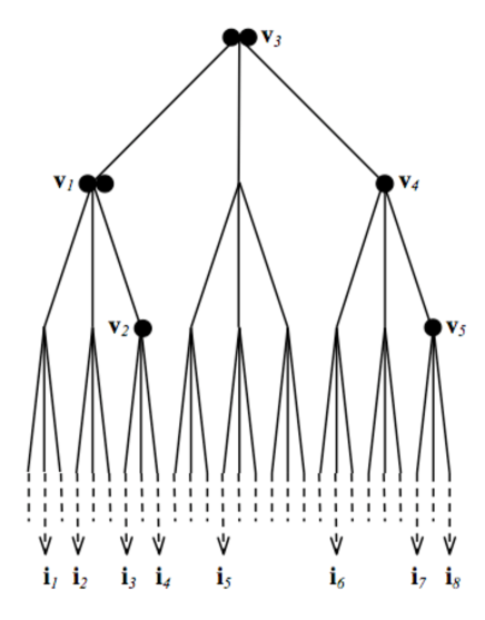
Figure 1: The join set $\{{\bf v}_{1},{\bf v}_{1},{\bf v}_{2},{\bf v}_{3},{\bf v}_{3},{\bf v}_{4},{\bf v}_{5}\}$ of $\{{\bf i}_{1},{\bf i}_{2},{\bf i}_{3},{\bf i}_{4},{\bf i}_{5},{\bf i}_{6},{\bf i}_{7},{\bf i}_{8}\}$

We define multienergy kernels by forming products of the singular value functions at the vertices of join sets. For ${\bf i}_{1},\ldots,{\bf i}_{n}\in I_{\infty}$ let

$$\phi^{s}({\bf i}_{1},\ldots,{\bf i}_{n})=\phi^{s}(T_{{\bf v}_{1}})\phi^{s}(T_{{\bf v}_{2}})\cdots\phi^{s}(T_{{\bf v}_{n-1}})\mbox{ where }\{{\bf v}_{1},\ldots,{\bf v}_{n-1}\}=\bigwedge({\bf i}_{1},\ldots,{\bf i}_{n}).$$ (5.2)

We will consider multienergy integrals of the form

$$\int\cdots\int\phi^{s}({\bf i}_{1},\ldots,{\bf i}_{n})^{-1}d\mu({\bf i}_{1})\ldots d\mu({\bf i}_{n})$$

which provide bounds for the expectation ${\sf E}\int\mu^{\omega}(B(x,r))^{q-1}d\mu^{\omega}(x)$.

The second stage involves showing that, for suitable $s$, certain multienergy integrals are finite, implying that $\int\mu^{\omega}(B(x,r))^{q-1}d\mu^{\omega}(x)<\infty$ almost surely, to give a lower bound for $\underline{D}_{q}\,(\mu^{w})$.

These two stages are executed in the next two sections.

6 Probabilistic estimates

The aim of this section is to bound the expectation of $\int\mu^{\omega}(B(x,r))^{q-1}d\mu^{\omega}(x)$, that is the integral which occurs in the definition of the generalised dimensions (3.4), in terms of a multienergy integral.

Let ${\sf E}$ denote expectation. Given $J\subseteq I$ we write ${\cal F}=\sigma\{\omega_{\bf i}:{\bf i}\in J\}$ for the sigma-field generated by the random displacements $\omega_{\bf i}\in J$ and write ${\sf E}(Z\mid{\cal F})$ for the expectation of a random variable $Z$ conditional on ${\cal F}$; intuitively this is the expectation of $Z$ given all the displacements $\{\omega_{\bf i}:{\bf i}\in J\}$.

Note that the constant $c$ may differ in each of the following lemmas. The first lemma is a ‘transversality’ property of a form often encountered in work on self-affine sets.

Lemma 6.1

Let $0<s\leq N$ with $s$ not an integer. Then there exists $c>0$ such that

$${\sf E}(|\Pi^{\omega}({\bf u})-\Pi^{\omega}({\bf v})|^{-s}\mid{\cal F})\leq c\phi^{s}(T_{{\bf u}\wedge{\bf v}})^{-1}$$

for all ${\bf u},{\bf v}\in I$, where ${\cal F}=\sigma\{\omega_{\bf i}:{\bf i}\in J\}$ for any subset $J$ of $T$ such that ${\bf v}|_{k+1},{\bf v}|_{k+2},\ldots\in J$ and ${\bf u}|_{k+2},{\bf u}|_{k+3},\ldots\in J$ but ${\bf u}|_{k+1}\notin J$, where $|{\bf u}\wedge{\bf v}|=k$.

Proof. From (2.7), for each ${\bf u},{\bf v}$,

$$\Pi^{\omega}({\bf u})-\Pi^{\omega}({\bf v})=T_{{\bf u}\wedge{\bf v}}\big{(}( \omega_{{\bf u}|_{k+1}}+T_{{\bf u}|_{k+1}}\omega_{{\bf u}|_{k+2}}+T_{{\bf u}|_{k+1}}T_{{\bf u}|_{k+2}}\omega_{{\bf u}|_{k+3}}+\cdots)$$

$$-(\omega_{{\bf v}|_{k+1}}+T_{{\bf v}|_{k+1}}\omega_{{\bf v}|_{k+2}}+T_{{\bf v}|_{k+1}}T_{{\bf v}|_{k+2}}\omega_{{\bf v}|_{k+3}}+\cdots)\big{)}$$

$$=T_{{\bf u}\wedge{\bf v}}\big{(}( \omega_{{\bf u}|_{k+1}}+x(\omega)\big{)}$$

where $x(\omega)$ is ${\cal F}$-measurable. Thus

$${\sf E}(|\Pi^{\omega}({\bf u})-\Pi^{\omega}({\bf v})|^{-s}\mid{\cal F})= \int\frac{d{\sf P}(\omega_{{\bf u}|_{k+1}})}{|T_{{\bf u}\wedge{\bf v}}\big{(}(\omega_{{\bf u}|_{k+1}}+x(\omega)\big{)}|^{s}}$$

$$\leq c\phi^{s}(T_{{\bf u}\wedge{\bf v}})^{-1},$$

where the integral may be estimated just as in [5, Lemma 3.1] or [15, Lemmas 4.5, 5.2]. $\Box$

We next use a sequence of conditional expectations to extend Lemma 6.1 from $2$ to $n+1$ points of $I_{\infty}$.

Lemma 6.2

For all $0<s\leq N$ with $s$ not an integer, there exist numbers $c>0$ and $r_{0}>0$ such that for all ${\bf i}_{1},\ldots,{\bf i}_{n},{\bf j}\in I_{\infty}$ and $0<r\leq r_{0}$,

$${\sf P}\big{\{}|\Pi^{\omega}({\bf i}_{1})-\Pi^{\omega}({\bf j})|\leq r,\ldots,|\Pi^{\omega}({\bf i}_{n})-\Pi^{\omega}({\bf j})|\leq r\big{\}}\leq cr^{sn}\phi^{s}({\bf i}_{1},\ldots,{\bf i}_{n},{\bf j})^{-1}.$$ (6.1)

Proof. We may renumber the points ${\bf i}_{1},\ldots,{\bf i}_{n}$ in such a manner that $\{{\bf i}_{1}\wedge{\bf i}_{2},{\bf i}_{2}\wedge{\bf i}_{3},\ldots,{\bf i}_{n-1}\wedge{\bf i}_{n},{\bf i}_{n}\wedge{\bf j}\}$ are precisely the points of the join set $\bigwedge({\bf i}_{1},\ldots,{\bf i}_{n})$, including any repeated points. (One way to achieve this renumbering is to transform the tree $I$ by an automorphism fixing the root $\emptyset$ in such a way that ${\bf j}$ is the ‘extreme right’ point of the tree and renumber the ${\bf i}_{k}$ from left to right.) Note that this renumbering does not affect the value of $\phi^{s}({\bf i}_{1},\ldots,{\bf i}_{n},{\bf j})$. Thus

$${\sf P}\big{\{} |\Pi^{\omega}({\bf i}_{1})-\Pi^{\omega}({\bf j})|\leq r,\ldots,|\Pi^{\omega}({\bf i}_{n})-\Pi^{\omega}({\bf j})|\leq r\big{\}}$$

$$\leq{\sf P}\big{\{}|\Pi^{\omega}({\bf i}_{1})-\Pi^{\omega}({\bf i}_{2})|\leq 2r,\ldots,|\Pi^{\omega}({\bf i}_{n-1})-\Pi^{\omega}({\bf i}_{n})|\leq 2r,|\Pi^{\omega}({\bf i}_{n})-\Pi^{\omega}({\bf j})|\leq 2r\big{\}}$$

$$\leq 2^{n}r^{sn}{\sf E}\big{(}|\Pi^{\omega}({\bf i}_{1})-\Pi^{\omega}({\bf i}_{2})|^{-s}\cdots|\Pi^{\omega}({\bf i}_{n-1})-\Pi^{\omega}({\bf i}_{n})|^{-s}|\Pi^{\omega}({\bf i}_{n})-\Pi^{\omega}({\bf j})|^{-s}\big{)}.$$ (6.2)

We estimate this expectation through a tower of conditional expectations. Define a sequence of sigma-fields ${\cal F}_{1}\supset{\cal F}_{2}\supset\cdots\supset{\cal F}_{n}$ by ${\cal F}_{l}=\sigma\{\omega_{\bf i}:{\bf i}\neq{\bf i}_{1}|_{k_{1}+1},\ldots,{\bf i}_{l}|_{k_{l}+1}\}$ where $k_{l}=|{\bf i}_{l}\wedge{\bf i}_{l+1}|\,(1\leq l\leq n-1)$ and $k_{n}=|{\bf i}_{n}\wedge{\bf j}|$.

For brevity of notation, write $Z^{\omega}_{l}=|\Pi^{\omega}({\bf i}_{l})-\Pi^{\omega}({\bf i}_{l+1})|^{-s}\,(1\leq l\leq n-1)$ with $Z^{\omega}_{n}=|\Pi^{\omega}({\bf i}_{n})-\Pi^{\omega}({\bf j})|^{-s}$, so that $Z^{\omega}_{l+1},\ldots,Z^{\omega}_{n}$ are all ${\cal F}_{l}$-measurable for $l=1,\ldots,n-1$. Using the tower property for conditional expectation, that $Z^{\omega}_{2}\ldots Z^{\omega}_{n}$ is ${\cal F}_{1}$-measurable, and then applying Lemma 6.1,

$${\sf E}\big{(}Z^{\omega}_{1}\ldots Z^{\omega}_{n}\big{|}{\cal F}_{n}\big{)} ={\sf E}\Big{(}{\sf E}\big{(}Z^{\omega}_{1}\ldots Z^{\omega}_{n}\big{|}{\cal F}_{1}\big{)}\big{|}{\cal F}_{n}\Big{)}$$

$$={\sf E}\Big{(}{\sf E}\big{(}Z^{\omega}_{1}\big{|}{\cal F}_{1}\big{)}Z^{\omega}_{2}\ldots Z^{\omega}_{n}\big{|}{\cal F}_{n}\Big{)}$$

$$\leq{\sf E}\big{(}c\phi^{s}(T_{{\bf i}_{1}\wedge{\bf i}_{2}})^{-1}Z^{\omega}_{2}\ldots Z^{\omega}_{n}\big{|}{\cal F}_{n}\big{)}$$

$$=c\phi^{s}(T_{{\bf i}_{1}\wedge{\bf i}_{2}})^{-1}{\sf E}\big{(}Z^{\omega}_{2}\ldots Z^{\omega}_{n}\big{|}{\cal F}_{n}\big{)}.$$

Repeating this argument $n-1$ times, we obtain that

$${\sf E}\big{(}Z^{\omega}_{1}\ldots Z^{\omega}_{n}\big{|}{\cal F}_{n}\big{)}\leq c^{n}\phi^{s}(T_{{\bf i}_{1}\wedge{\bf i}_{2}})^{-1}\ldots\phi^{s}(T_{{\bf i}_{n-1}\wedge{\bf i}_{n}})^{-1}\phi^{s}(T_{{\bf i}_{n}\wedge{\bf j}})^{-1}=c^{n}\phi^{s}({\bf i}_{1},\ldots,{\bf i}_{n},{\bf j})^{-1},$$

giving the bound for the unconditional expectation

$${\sf E}\big{(}|\Pi^{\omega}({\bf i}_{1})-\Pi^{\omega}({\bf i}_{2})|^{-s} \cdots|\Pi^{\omega}({\bf i}_{n-1})-\Pi^{\omega}({\bf i}_{n})|^{-s}|\Pi^{\omega}({\bf i}_{n})-\Pi^{\omega}({\bf j})|^{-s}\big{)}$$

$$={\sf E}\big{(}Z^{\omega}_{1}\ldots Z^{\omega}_{n})\leq c^{n}\phi^{s}({\bf i}_{1},\ldots,{\bf i}_{n},{\bf j})^{-1}.$$

Combining this with (6.2) gives (6.1). $\Box$

We now integrate (6.1) over the ${\bf i}_{l}$.

Lemma 6.3

For all $0<s\leq N$ with $s$ not an integer, there exist numbers $c>0$ and $r_{0}>0$ such that for all ${\bf j}\in I_{\infty}$ and $0<r\leq r_{0}$,

$${\sf E}\big{(}\mu^{\omega}(B(\Pi^{\omega}({\bf j}),r))^{n}\big{)}\leq cr^{sn}\int\cdots\int\phi^{s}({\bf i}_{1},\ldots,{\bf i}_{n},{\bf j})^{-1}d\mu({\bf i}_{1})\ldots d\mu({\bf i}_{n}).$$ (6.3)

Proof. Using Fubini’s theorem,

$${\sf E}\big{(}\mu^{\omega} (B(\Pi^{\omega}({\bf j}),r))^{n}\big{)}$$

$$={\sf E}\big{(}\mu\{{\bf i}:|\Pi^{\omega}({\bf i})-\Pi^{\omega}({\bf j})|\leq r\}^{n}\big{)}$$

$$=\big{(}{\sf P}\times\mu\times\cdots\times\mu\big{)}\big{\{}(\omega,{\bf i}_{1},\ldots,{\bf i}_{n}):|\Pi^{\omega}({\bf i}_{1})-\Pi^{\omega}({\bf j})|\leq r,\ldots,|\Pi^{\omega}({\bf i}_{n})-\Pi^{\omega}({\bf j})|\leq r\big{\}}$$

$$=\int\cdots\int{\sf P}\big{\{}|\Pi^{\omega}({\bf i}_{1})-\Pi^{\omega}({\bf j})|\leq r,\ldots,|\Pi^{\omega}({\bf i}_{n})-\Pi^{\omega}({\bf j})|\leq r\big{\}}d\mu({\bf i}_{1})\ldots d\mu({\bf i}_{n})$$

$$\leq cr^{sn}\int\cdots\int\phi^{s}({\bf i}_{1},\ldots,{\bf i}_{n},{\bf j})^{-1}d\mu({\bf i}_{1})\ldots d\mu({\bf i}_{n}),$$

by Lemma 6.2. $\Box$

Finally, integration of an appropriate power of (6.3) with respect to ${\bf j}$ gives the main estimate (note the simpler form of (6.4) if $q=n+1$ is an integer).

Proposition 6.4

Let $n\geq 1$ and $1<q\leq n+1$. Then for all $0<s\leq N$ with $s$ not an integer, there exist numbers $c>0$ and $r_{0}>0$ such that for all $0<r\leq r_{0}$,

$${\sf E}\int\mu^{\omega} (B(x,r))^{q-1}d\mu^{\omega}(x)$$

$$\leq cr^{s(q-1)}\int\bigg{[}\int\cdots\int\phi^{s}({\bf i}_{1},\ldots,{\bf i}_{n},{\bf j})^{-1}d\mu({\bf i}_{1})\ldots d\mu({\bf i}_{n})\bigg{]}^{(q-1)/n}d\mu({\bf j})$$ (6.4)

Proof. Since $n/(q-1)\geq 1$, Jensen’s inequality and (6.3) give

$${\sf E}\int\mu^{\omega}(B(x, r))^{q-1}d\mu^{\omega}(x)$$

$$={\sf E}\int\mu^{\omega}(B(\Pi^{\omega}({\bf j}),r))^{q-1}d\mu({\bf j})$$

$$\leq\int\Big{[}{\sf E}\big{(}\mu^{\omega}(B(\Pi^{\omega}({\bf j}),r))^{n}\big{)}\Big{]}^{(q-1)/n}d\mu({\bf j})$$

$$\leq cr^{s(q-1)}\int\bigg{[}\int\cdots\int\phi^{s}({\bf i}_{1},\ldots,{\bf i}_{n},{\bf j})^{-1}d\mu({\bf i}_{1})\ldots d\mu({\bf i}_{n})\bigg{]}^{(q-1)/n}d\mu({\bf j}).$$

$\Box$

7 Integral estimates

This section is devoted to estimating the integral (6.4). To do this we identify the code space $I$ with the vertices of a rooted $m$-ary tree with root $\emptyset$, in the obvious way. Thus the edges of the tree join each ${\bf i}\in I$ to its $m$ ‘children’ ${\bf i}1,\ldots,{\bf i}m$. To estimate (6.4) we will split the domain of integration into subdomains consisting of $n$-tuples $({\bf i}_{1},\ldots,{\bf i}_{n})$ whose join sets lie in certain families of automorphisms of the tree $I$. We will use induction over classes of join sets to estimate the integrals over each such domain, with Hölder’s inequality playing a very natural rôle at each step.

We require a little terminology. A join set $J$ with root ${\bf w}\in I$ consists of a family of vertices $\{{\bf v}_{1},\ldots,{\bf v}_{r}\}$ of $I$, with repetitions allowed, such that ${\bf v}_{i}\succeq{\bf w}$ for all $i$ and with the property that ${\bf v}_{i}\wedge{\bf v}_{j}\in J$ for all ${\bf v}_{i},{\bf v}_{j}\in J$. The root may or may not be a vertex of the join set. The number $r+1$ is called the spread of the join set. The multiplicity of a given vertex is the number of times it occurs in $J$.

Join sets occur naturally in connection with the integrals (6.4): given ${\bf i}_{1},\ldots,{\bf i}_{n}\in I_{\infty}$ then $J=\bigwedge({\bf i}_{1},\ldots,{\bf i}_{n})$ is a join set of spread $n$, and the multiplicity of a vertex ${\bf v}\in J$ is $r-1$ where $r$ is the greatest integer such that there are distinct ${\bf i}_{i_{1}},\ldots,{\bf i}_{i_{r}}$ with ${\bf i}_{i_{p}}\wedge{\bf i}_{i_{q}}={\bf v}$ for all $1\leq p<q\leq r$. (In a binary tree every vertex of a join set has multiplicity 1.)

A join class ${\cal J}$ with root ${\bf w}\in I$ is an equivalence class of join sets all with root ${\bf w}$, two such join sets $J$ and $J^{\prime}$ being equivalent if there is an automorphism of the rooted subtree of $I$ with root ${\bf w}$ that maps $J$ onto $J^{\prime}$ (preserving multiplicities). The spread of a join class ${\cal J}$ is the common value of the spreads of all $J\in{\cal J}$.

The level of a vertex ${\bf v}\in I$ is just $|{\bf v}|$. Thus the set of levels $L(J)$ of a join set $J=\{{\bf v}_{1},\ldots,{\bf v}_{r}\}$ is $\{|{\bf v}_{1}|,\ldots,|{\bf v}_{r}|\}$, allowing repetitions, and the set of levels $L({\cal J})$ of a join class is the common set of levels of the join sets in the class.

Note that in (7.1) and below, the product is over the set of levels in a join class. The symbol $[n-1]$ above the product sign merely indicates that there are $n-1$ terms in this product; this convention is helpful when keeping track of terms through the proofs.

Proposition 7.1

Let $q>1$ and $n\geq 2$ be such that $q\geq n$. Let ${\cal J}$ be a join class with root ${\bf v}$ and spread $n$. Then

$$\int_{\bigwedge({\bf i}_{1},\ldots,{\bf i}_{n})\in{\cal J}} \phi^{s}({\bf i}_{1},\ldots,{\bf i}_{n})^{-1}d\mu({\bf i}_{1})\ldots d\mu({\bf i}_{n})$$

$$\leq\mu(C_{\bf v})^{(q-n)/(q-1)}\prod_{l\in L({\cal J})}^{[n-1]}\Big{(}\sum_{|{\bf u}|=l,{\bf u}\succeq{\bf v}}\phi^{s}(T_{\bf u})^{1-q}\mu(C_{{\bf u}})^{q}\Big{)}^{1/(q-1)}.$$ (7.1)

Proof. We proceed by induction on the number of distinct vertices of ${\cal J}$. To start the inductive process, suppose that the join sets in ${\cal J}$ consist of a single vertex ${\bf v}$ of multiplicity $n-1$ for some $n\geq 2$. First assume that ${\bf v}$ is itself the root of the join sets of ${\cal J}$. Then

$$\int_{\bigwedge({\bf i}_{1},\ldots,{\bf i}_{n})\in{\cal J}}\phi^{s}({\bf i}_{1},\ldots,{\bf i}_{n})^{-1} d\mu({\bf i}_{1})\ldots d\mu({\bf i}_{n})=\int_{\bigwedge({\bf i}_{1},\ldots,{\bf i}_{n})\in{\cal J}}\phi^{s}(T_{\bf v})^{-(n-1)}d\mu({\bf i}_{1})\ldots d\mu({\bf i}_{n})$$

$$\leq\phi^{s}(T_{\bf v})^{-(n-1)}\mu(C_{\bf v})^{n}$$

$$=\mu(C_{\bf v})^{(q-n)/(q-1)}\big{(}\phi^{s}(T_{\bf v})^{1-q}\mu(C_{\bf v})^{q}\big{)}^{(n-1)/(q-1)},$$ (7.2)

which is (7.1), noting that $L({\cal J})$ has just one level $|{\bf v}|$ which is of multiplicity $n-1$, with the sums in each multiplicand of (7.1) having just one term each.

If, now, the join class ${\cal J}$ has root ${\bf w}$ and contains join sets $J$ consisting of a single vertex ${\bf v}$, distinct from ${\bf w}$, of multiplicity $n-1$ at level $l$, we may sum (7.2) over ${\bf v}$ such that ${\bf v}\succeq{\bf w}$ and $|{\bf v}|=l$ to get, using Hölder’s inequality,

$$\int_{\bigwedge({\bf i}_{1},\ldots,{\bf i}_{n})\in{\cal J}} \phi^{s}({\bf i}_{1},\ldots,{\bf i}_{n})^{-1}d\mu({\bf i}_{1})\ldots d\mu({\bf i}_{n})$$

$$\leq\sum_{|{\bf v}|=l,{\bf v}\succeq{\bf w}}\mu(C_{\bf v})^{(q-n)/(q-1)}\big{(}\phi^{s}(T_{\bf v})^{1-q}\mu(C_{\bf v})^{q}\big{)}^{(n-1)/(q-1)}$$

$$\leq\Big{(}\sum_{|{\bf v}|=l,{\bf v}\succeq{\bf w}}\mu(C_{\bf v})\Big{)}^{(q-n)/(q-1)}\Big{(}\sum_{|{\bf v}|=l,{\bf v}\succeq{\bf w}}\phi^{s}(T_{\bf v})^{1-q}\mu(C_{\bf v})^{q}\Big{)}^{(n-1)/(q-1)}$$

$$=\mu(C_{\bf w})^{(q-n)/(q-1)}\Big{(}\sum_{|{\bf v}|=l,{\bf v}\succeq{\bf w}}\phi^{s}(T_{\bf v})^{1-q}\mu(C_{\bf v})^{q}\Big{)}^{(n-1)/(q-1)},$$

which is (7.1) for join classes with a single vertex of any multiplicity.

Now assume inductively that (7.1) holds for all join sets with fewer than $k$ distinct vertices for some $k\geq 2$. Let ${\cal J}$ be a join class with root ${\bf v}$ and $k\geq 2$ distinct vertices and spread $n$ where $n\leq q$. Again, first consider the case where that the root ${\bf v}$ belongs to the join sets in ${\cal J}$ as the ‘top’ vertex. In each join set $J\in{\cal J}$ there is a (possibly empty) set of $r\geq 0$ vertices $\{{\bf v}_{1},\ldots,{\bf v}_{r}\}$ in $J$ distinct from and ‘immediately below’ ${\bf v}$, that is with the path joining ${\bf v}_{i}$ to ${\bf v}$ in the tree $I$ containing no other vertices of $J$. For a given class ${\cal J}$ these sets of vertices (with multiplicity) are equivalent under automorphisms of the tree that fix the root ${\bf v}$.

For each $i$, the join set $J\in{\cal J}$ induces a join set that we denote by $J_{i}$ with root ${\bf v}$ and vertices $\{{\bf u}\in J:{\bf u}\succeq{\bf v}_{i}\}$, that is the vertices of ${\cal J}$ below and including ${\bf v}_{i}$. These join sets are equivalent under automorphisms of the tree that fix the root ${\bf v}$ and we write ${\cal J}_{i}=\{J_{i}:J\in{\cal J}\}$ for this equivalence class of join sets, which has spread $n_{i}\geq 2$, say, and set of levels $L_{i}$ (counted with repetitions).

Let

$$n_{1}+\cdots+n_{r}+t=n,$$ (7.3)

where $t\geq 0$. To integrate over $\{{\bf i}_{1},\ldots,{\bf i}_{n}\}$ such that $\bigwedge({\bf i}_{1},\ldots,{\bf i}_{n})\in{\cal J}$ we decompose the integral so that for each $J\in{\cal J}$, for each $i\,(1\leq i\leq r)$, the $n_{i}$ integration variables, $\{{\bf i}_{1}^{i},\ldots,{\bf i}_{n_{i}}^{i}\}$ say, are such that $\bigwedge({\bf i}_{1}^{i},\ldots,{\bf i}_{n_{i}}^{i})=J_{i}$, and $t$ of them, $\{{\bf i}_{1}^{0},\ldots,{\bf i}_{t}^{0}\}$, such that ${\bf i}_{l}^{0}\wedge{\bf i}_{r}={\bf v}$ for all ${\bf i}_{r}\neq{\bf i}_{l}^{0}$. Thus, noting that the multiplicity of ${\bf v}$ is $r+t-1$,

$$I \equiv\int_{\bigwedge({\bf i}_{1},\ldots,{\bf i}_{n})\in{\cal J}}\phi^{s}({\bf i}_{1},\ldots,{\bf i}_{n})^{-1}d\mu({\bf i}_{1})\ldots d\mu({\bf i}_{n})$$

$$\leq\phi^{s}(T_{\bf v})^{-(r+t-1)}\mu(C_{\bf v})^{t}\int_{\bigwedge({\bf i}_{1}^{1},\ldots,{\bf i}_{n_{1}}^{1})\in{\cal J}_{1}}\phi^{s}({\bf i}_{1}^{1},\ldots,{\bf i}_{n_{1}}^{1})^{-1}d\mu({\bf i}_{1}^{1})\ldots d\mu({\bf i}_{n_{1}}^{1})$$

$$\quad\quad\times\cdots\times\int_{\bigwedge({\bf i}_{1}^{r},\ldots,{\bf i}_{n_{r}}^{r})\in{\cal J}_{r}}\phi^{s}({\bf i}_{1}^{r},\ldots,{\bf i}_{n_{r}}^{r})^{-1}d\mu({\bf i}_{1}^{r})\ldots d\mu({\bf i}_{n_{r}}^{r})$$

$$\leq\phi^{s}(T_{\bf v})^{1-r-t}\mu(C_{\bf v})^{t}\mu(C_{{\bf v}})^{(q-n_{1})/(q-1)}\prod_{l\in L_{1}}^{[n_{1}-1]}\Big{(}\sum_{|{\bf u}|=l,{\bf u}\succeq{\bf v}}\phi^{s}(T_{\bf u})^{1-q}\mu(C_{{\bf u}})^{q}\Big{)}^{1/(q-1)}$$

$$\quad\quad\times\cdots\times\mu(C_{{\bf v}})^{(q-n_{r})/(q-1)}\prod_{l\in L_{r}}^{[n_{r}-1]}\Big{(}\sum_{|{\bf u}|=l,{\bf u}\succeq{\bf v}}\phi^{s}(T_{\bf u})^{1-q}\mu(C_{{\bf u}})^{q}\Big{)}^{1/(q-1)},$$

where we have applied the inductive assumption (7.1) to join sets in ${\cal J}_{i}$ (which all have root ${\bf v}$) for each $i$.

Combining terms,

$$I \leq\mu(C_{{\bf v}})^{(q-n_{1}-\cdots-n_{r}-t)/(q-1)}\big{(}\phi^{s}(T_{\bf v})^{1-q}\mu(C_{\bf v})^{q}\big{)}^{(r+t-1)/(q-1)}$$

$$\qquad\qquad\qquad\qquad\qquad\times\prod_{l\in L_{1}\cup\cdots\cup L_{r}}^{[n_{1}+\cdots+n_{r}-r]}\Big{(}\sum_{|{\bf u}|=l,{\bf u}\succeq{\bf v}}\phi^{s}(T_{\bf u})^{1-q}\mu(C_{{\bf u}})^{q}\Big{)}^{1/(q-1)}$$

$$\leq\mu(C_{{\bf v}})^{(q-n)/(q-1)}\prod_{l\in L}^{[n-1]}\Big{(}\sum_{|{\bf u}|=l,{\bf u}\succeq{\bf v}}\phi^{s}(T_{\bf u})^{1-q}\mu(C_{{\bf u}})^{q}\Big{)}^{1/(q-1)},$$

where $L$ is the complete set of levels of ${\cal J}$, where we have used (7.3), and incorporated the terms $\phi^{s}(T_{\bf v})^{1-q}\mu(C_{\bf v})^{q}$ (taken as a sum over the single vertex ${\bf v}$) in the main product with multiplicity $(r+t-1)$. This is (7.1) in the case where the root of the join sets in ${\cal J}$ belongs to the join sets.

Finally, if the root ${\bf w}$ is not a vertex of the join sets in ${\cal J}$, then summing (7.1) over join sets with top vertex ${\bf v}\preceq{\bf w}$ with $|{\bf v}|=l^{\prime}$ and using Hölder’s inequality,

$$\int_{\bigwedge({\bf i}_{1},\ldots,{\bf i}_{n})\in{\cal J}} \phi^{s}({\bf i}_{1},\ldots,{\bf i}_{n})^{-1}d\mu({\bf i}_{1})\ldots d\mu({\bf i}_{n})$$

$$\leq\sum_{|{\bf v}|=l^{\prime},{\bf v}\succeq{\bf w}}\mu(C_{\bf v})^{(q-n)/(q-1)}\prod_{l\in L({\cal J})}^{[n-1]}\Big{(}\sum_{|{\bf u}|=l,{\bf u}\succeq{\bf v}}\phi^{s}(T_{\bf u})^{1-q}\mu(C_{{\bf u}})^{q}\Big{)}^{1/(q-1)}$$

$$\leq\Big{(}\sum_{|{\bf v}|=l^{\prime},{\bf v}\succeq{\bf w}}\mu(C_{\bf v})\Big{)}^{(q-n)/(q-1)}\prod_{l\in L({\cal J})}^{[n-1]}\Big{(}\sum_{|{\bf v}|=l^{\prime},{\bf v}\succeq{\bf w}}\sum_{|{\bf u}|=l,{\bf u}\succeq{\bf v}}\phi^{s}(T_{\bf u})^{1-q}\mu(C_{{\bf u}})^{q}\Big{)}^{1/(q-1)}$$

$$=\mu(C_{\bf w})^{(q-n)/(q-1)}\prod_{l\in L({\cal J})}^{[n-1]}\Big{(}\sum_{|{\bf u}|=l,{\bf u}\succeq{\bf w}}\phi^{s}(T_{\bf u})^{1-q}\mu(C_{{\bf u}})^{q}\Big{)}^{1/(q-1)},$$

which completes the induction and the proof. $\Box$

Proposition 7.1 would be adequate for our needs for the cases when $q$ is an integer. However for non-integral $q>1$ we need a generalisation where one of the variables of integration is distinguished. Whilst the proof of Proposition 7.2 again uses induction on join sets and Hölder’s inequality, the details are more intricate than in Proposition 7.1, and indeed depends on Proposition 7.1 at several points.

Let $0\leq k_{1}<k_{2}<\ldots<k_{p}$ be levels, where $1\leq p\leq n$. For ${\bf j}\in I_{\infty}$ write ${\bf j}_{r}={\bf j}|_{k_{r}}$. For each $r=1,\ldots,p$, let ${\cal J}_{r}$ be a given join class with root at level $k_{r}$ and spread $m_{r}$, see Figure 2. Write ${\cal J}_{r}({\bf j}_{r})$ for the corresponding join class with the root mapped to ${\bf j}_{r}$, that is so that the tree automorphisms of $I$ that map ${\bf j}_{r}$ to ${\bf j}_{r}^{\prime}$ map the join sets in ${\cal J}_{r}({\bf j}_{r})$ onto those in ${\cal J}_{r}({\bf j}_{r}^{\prime})$ in a bijective manner.

We need to include the cases where ${\cal J}_{r}({\bf j}_{r})$ is a join class with root ${\bf j}_{r}$ and of spread $1$. In this case we interpret integration over $\bigwedge({\bf i}_{l})\in{\cal J}_{r}({\bf j}_{r})$ as integration over all ${\bf i}_{l}$ such that ${\bf i}_{l}\wedge{\bf j}={\bf j}_{r}$, and we take $\phi^{s}({\bf i}_{l})=1$ where this occurs in the next proof.

Proposition 7.2

Let $q>1$ and let $n$ be an integer with $n\geq q-1$. With notation as above, for each $r=1,\ldots,p$ let ${\cal J}_{r}$ be a join class with root at level $k_{r}$ and spread $m_{r}\geq 1$, with $m_{1}+\cdots+m_{p}=n$. Then

$$\int_{{\bf j}\in I}\bigg{[}\int_{\bigwedge({\bf i}_{1},\ldots,{\bf i}_{m_{1}})\in{\cal J}_{1}({\bf j}_{1})}\cdots\int_{\bigwedge({\bf i}_{n-m_{p}+1},\ldots,{\bf i}_{n})\in{\cal J}_{p}({\bf j}_{p})} \phi^{s}({\bf i}_{1},\ldots,{\bf i}_{n},{\bf j})^{-1}d\mu({\bf i}_{1})\ldots d\mu({\bf i}_{n})\bigg{]}^{(q-1)/n}d\mu({\bf j})$$

$$\leq\prod_{l\in L}^{[n]}\Big{(}\sum_{|{\bf u}|=l}\phi^{s}(T_{\bf u})^{1-q}\mu(C_{{\bf u}})^{q}\Big{)}^{1/n},$$ (7.4)

where $L$ denotes the aggregate set of levels of $\{L({\cal J}_{1}),\ldots,L({\cal J}_{p}),k_{1},\ldots,k_{p}\}$.

Proof. We proceed by induction on $r$, starting with $r=p$ and working up to $r=1$, taking as the inductive hypothesis:

For all ${\bf j}_{r}\in I_{k_{r}}$,

$$\int_{{\bf j}\succeq{\bf j}_{r}}\bigg{[} \int_{\bigwedge({\bf i}^{r}_{1},\ldots,{\bf i}^{r}_{m_{r}})\in{\cal J}_{r}({\bf j}_{r})}\cdots\int_{\bigwedge({\bf i}^{p}_{1},\ldots,{\bf i}^{p}_{m_{p}})\in{\cal J}_{p}({\bf j}_{p})}\phi^{s}({\bf i}^{r}_{1},\ldots,{\bf i}^{r}_{m_{r}})^{-1}\phi^{s}(T_{{\bf j}_{r}})^{-1}\times\cdots$$

$$\qquad\times\phi^{s}({\bf i}^{p}_{1},\ldots,{\bf i}^{p}_{m_{p}})^{-1}\phi^{s}(T_{{\bf j}_{p}})^{-1}d\mu({\bf i}^{r}_{1})\ldots d\mu({\bf i}^{r}_{m_{r}})\cdots d\mu({\bf i}^{p}_{1})\ldots d\mu({\bf i}^{p}_{m_{p}})\bigg{]}^{(q-1)/n}d\mu({\bf j})$$

$$\leq\mu(C_{{\bf j}_{r}})^{(n-n_{r})/n}\prod_{l\in L_{r}}^{[n_{r}]}\Big{(}\sum_{|{\bf u}|=l,{\bf u}\succeq{\bf j}_{r}}\phi^{s}(T_{\bf u})^{1-q}\mu(C_{{\bf u}})^{q}\Big{)}^{1/n},$$ (7.5)

where $n_{r}=m_{r}+\cdots+m_{p}$ and $L_{r}$ denotes the set of levels of $\{L({\cal J}_{r}),\ldots,L({\cal J}_{p}),k_{r},\ldots,k_{p}\}$ counted by multiplicity (so that $L_{r}$ consists of $m_{r}+\cdots+m_{p}=n_{r}-1$ levels).

Figure 2: Part of the tree $I$ indicating the notation of Proposition 7.2

To start the induction, we apply Proposition 7.1 to get

$$\int_{{\bf j}\succeq{\bf j}_{p}} \bigg{[}\int_{\bigwedge({\bf i}^{p}_{1},\ldots,{\bf i}^{p}_{m_{p}})\in{\cal J}_{p}({\bf j}_{p})}\phi^{s}({\bf i}^{p}_{1},\ldots,{\bf i}^{p}_{m_{p}})^{-1}\phi^{s}(T_{{\bf j}_{p}})^{-1}d\mu({\bf i}^{p}_{1})\ldots d\mu({\bf i}^{p}_{m_{p}})\bigg{]}^{(q-1)/n}d\mu({\bf j})$$ (7.6)

$$\leq\int_{{\bf j}\succeq{\bf j}_{p}}\bigg{[}\mu(C_{{\bf j}_{p}})^{(q-m_{p})/(q-1)}\phi^{s}(T_{{\bf j}_{p}})^{-1}\prod_{l\in L({\cal J}_{p}({\bf j}_{p}))}^{[m_{p}-1]}\Big{(}\sum_{|{\bf u}|=l,{\bf u}\succeq{\bf j}_{p}}\phi^{s}(T_{\bf u})^{1-q}\mu(C_{{\bf u}})^{q}\Big{)}^{1/(q-1)}\bigg{]}^{(q-1)/n}d\mu({\bf j})$$

$$=\mu(C_{{\bf j}_{p}})^{(n-m_{p})/n}\big{(}\phi^{s}(T_{{\bf j}_{p}})^{1-q}\mu(C_{{\bf j}_{p}})^{q}\big{)}^{1/n}\prod_{l\in L({\cal J}_{p}({\bf j}_{p}))}^{[m_{p}-1]}\Big{(}\sum_{|{\bf u}|=l,{\bf u}\succeq{\bf j}_{p}}\phi^{s}(T_{\bf u})^{1-q}\mu(C_{{\bf u}})^{q}\Big{)}^{1/n}$$

$$=\mu(C_{{\bf j}_{p}})^{(n-n_{p})/n}\prod_{l\in L_{r}}^{[n_{p}]}\Big{(}\sum_{|{\bf u}|=l,{\bf u}\succeq{\bf j}_{p}}\phi^{s}(T_{\bf u})^{1-q}\mu(C_{{\bf u}})^{q}\Big{)}^{1/n},$$

on incorporating $(\phi^{s}(T_{{\bf j}_{p}})^{1-q}\mu(C_{{\bf j}_{p}})^{q})^{1/n}$ in the main product and noting that $m_{p}=n_{p}$. (Observe that this remains valid if $m_{p}=1$, in which case the inner integral in (7.6) is with respect to the single variable ${\bf i}^{p}_{1}$ over the cylinder $C_{{\bf j}_{p}}$, taking $\phi^{s}({\bf i}^{p}_{1})=1$.) This establishes the inductive hypothesis (7.5) when $r=p$.

Now assume that (7.5) is valid for $r=k,\ldots,p$ for some $2\leq k\leq p$. Then

$$I\equiv \int_{{\bf j}\succeq{\bf j}_{k-1}}\bigg{[}\int_{\bigwedge({\bf i}^{k-1}_{1},\ldots,{\bf i}^{k-1}_{m_{k-1}})\in{\cal J}_{k-1}({\bf j}_{k-1})}\int_{\bigwedge({\bf i}^{k}_{1},\ldots,{\bf i}^{k}_{m_{k}})\in{\cal J}_{k}({\bf j}_{k})}\cdots\int_{\bigwedge({\bf i}^{p}_{1},\ldots,{\bf i}^{p}_{m_{p}})\in{\cal J}_{p}({\bf j}_{p})}$$

$$\quad\Big{(}\phi^{s}({\bf i}^{k-1}_{1},\ldots,{\bf i}^{k-1}_{m_{k-1}})^{-1}\phi^{s}(T_{{\bf j}_{k-1}})^{-1}\phi^{s}({\bf i}^{k}_{1},\ldots,{\bf i}^{k}_{m_{k}})^{-1}\phi^{s}(T_{{\bf j}_{k}})^{-1}\cdots\phi^{s}({\bf i}^{p}_{1},\ldots,{\bf i}^{p}_{m_{p}})^{-1}\phi^{s}(T_{{\bf j}_{p}})^{-1}\Big{)}$$

$$\qquad\qquad\qquad d\mu({\bf i}^{k-1}_{1})\ldots d\mu({\bf i}^{k-1}_{m_{k-1}})d\mu({\bf i}^{k}_{1})\ldots d\mu({\bf i}^{k}_{m_{k}})\cdots d\mu({\bf i}^{p}_{1})\ldots d\mu({\bf i}^{p}_{m_{p}})\bigg{]}^{(q-1)/n}d\mu({\bf j})$$

$$=\phi^{s}(T_{{\bf j}_{k-1}})^{(1-q)/n}\bigg{[}\int_{\bigwedge({\bf i}^{k-1}_{1},\ldots,{\bf i}^{k-1}_{m_{k-1}})\in{\cal J}_{k-1}({\bf j}_{k-1})}\phi^{s}({\bf i}^{k-1}_{1},\ldots,{\bf i}^{k-1}_{m_{k-1}})^{-1}d\mu({\bf i}^{k-1}_{1})\ldots d\mu({\bf i}^{k-1}_{m_{k-1}})\bigg{]}^{(q-1)/n}$$

$$\qquad\times\sum_{{\bf j}_{k}\succeq{\bf j}_{k-1}}\int_{{\bf j}\succeq{\bf j}_{k}}\bigg{[}\int_{\bigwedge({\bf i}^{k}_{1},\ldots,{\bf i}^{k}_{m_{k}})\in{\cal J}_{k}({\bf j}_{k})}\cdots\int_{\bigwedge({\bf i}^{p}_{1},\ldots,{\bf i}^{p}_{m_{p}})\in{\cal J}_{p}({\bf j}_{p})}\Big{(}\phi^{s}({\bf i}^{k}_{1},\ldots,{\bf i}^{k}_{m_{k}})^{-1}\phi^{s}(T_{{\bf j}_{k}})^{-1}\times\cdots$$

$$\qquad\qquad\qquad\times\phi^{s}({\bf i}^{p}_{1},\ldots,{\bf i}^{p}_{m_{p}})^{-1}\phi^{s}(T_{{\bf j}_{p}})^{-1}\Big{)}d\mu({\bf i}^{k}_{1})\ldots d\mu({\bf i}^{k}_{m_{k}})\cdots d\mu({\bf i}^{p}_{1})\ldots d\mu({\bf i}^{p}_{m_{p}})\bigg{]}^{(q-1)/n}d\mu({\bf j})$$

$$\leq\phi^{s}(T_{{\bf j}_{k-1}})^{(1-q)/n}\bigg{[}\mu(C_{{\bf j}_{k-1}})^{(q-m_{k-1})/n}\prod_{l\in L({\cal J}_{k-1}({\bf j}_{k-1}))}^{[m_{k-1}-1]}\Big{(}\sum_{|{\bf u}|=l,{\bf u}\succeq{\bf j}_{k-1}}\phi^{s}(T_{\bf u})^{1-q}\mu(C_{{\bf u}})^{q}\Big{)}^{1/n}\bigg{]}$$

$$\qquad\qquad\times\sum_{{\bf j}_{k}\succeq{\bf j}_{k-1}}\mu(C_{{\bf j}_{k}})^{(n-n_{k})/n}\prod_{l\in L_{k}}^{[n_{k}]}\Big{(}\sum_{|{\bf u}|=l,{\bf u}\succeq{\bf j}_{k}}\phi^{s}(T_{\bf u})^{1-q}\mu(C_{{\bf u}})^{q}\Big{)}^{1/n},$$ (7.7)

where we have used Proposition 7.1 to estimate the first part and the inductive hypothesis (7.5) for the second part. Using Hölder’s inequality for each ${\bf j}_{k-1}$:

$$\sum_{{\bf j}_{k}\succeq{\bf j}_{k-1}} \mu(C_{{\bf j}_{k}})^{(n-n_{k})/n}\prod_{l\in L_{k}}^{[n_{k}]}\Big{(}\sum_{|{\bf u}|=l,{\bf u}\succeq{\bf j}_{k}}\phi^{s}(T_{\bf u})^{1-q}\mu(C_{{\bf u}})^{q}\Big{)}^{1/n}$$

$$\leq\Big{(}\sum_{{\bf j}_{k}\succeq{\bf j}_{k-1}}\mu(C_{{\bf j}_{k}})\Big{)}^{(n-n_{k})/n}\prod_{l\in L_{k}}^{[n_{k}]}\Big{(}\sum_{{\bf j}_{k}\succeq{\bf j}_{k-1}}\sum_{|{\bf u}|=l,{\bf u}\succeq{\bf j}_{k}}\phi^{s}(T_{\bf u})^{1-q}\mu(C_{{\bf u}})^{q}\Big{)}^{1/n}$$

$$=\mu(C_{{\bf j}_{k-1}})^{(n-n_{k})/n}\prod_{l\in L_{k}}^{[n_{k}]}\Big{(}\sum_{|{\bf u}|=l,{\bf u}\succeq{\bf j}_{k-1}}\phi^{s}(T_{\bf u})^{1-q}\mu(C_{{\bf u}})^{q}\Big{)}^{1/n}.$$

Thus from (7.7)

$$I\leq\mu (C_{{\bf j}_{k-1}})^{(n-n_{k}-m_{k-1})/n}\big{(}\phi^{s}(T_{{\bf j}_{k-1}})^{(1-q)}\mu(C_{{\bf j}_{k-1}})^{q}\big{)}^{1/n}$$

$$\times\prod_{l\in L({\cal J}_{k-1}({\bf j}_{k-1}))}^{[m_{k-1}-1]}\Big{(}\sum_{|{\bf u}|=l,{\bf u}\succeq{\bf j}_{k-1}}\phi^{s}(T_{\bf u})^{1-q}\mu(C_{{\bf u}})^{q}\Big{)}^{1/n}\prod_{l\in L_{k}}^{[n_{k}]}\Big{(}\sum_{|{\bf u}|=l,{\bf u}\succeq{\bf j}_{k-1}}\phi^{s}(T_{\bf u})^{1-q}\mu(C_{{\bf u}})^{q}\Big{)}^{1/n}$$

$$=\mu (C_{{\bf j}_{k-1}})^{(n-n_{k}-m_{k-1})/n}\prod_{l\in L_{k-1}}^{[m_{k-1}+n_{k}]}\Big{(}\sum_{|{\bf u}|=l,{\bf u}\succeq{\bf j}_{k-1}}\phi^{s}(T_{\bf u})^{1-q}\mu(C_{{\bf u}})^{q}\Big{)}^{1/n},$$

which is (7.5) with $r=k-1$, noting that $m_{k-1}+n_{k}=n_{k-1}$.

Finally, taking $r=1$ in (7.5) and noting that $n_{1}=n$,

$$\int_{{\bf j}\succeq{\bf j}_{1}}\bigg{[}\int_{\bigwedge({\bf i}_{1},\ldots,{\bf i}_{m_{1}})\in{\cal J}_{1}({\bf j}_{1})}\cdots\int_{\bigwedge({\bf i}_{n-m_{p}+1},\ldots,{\bf i}_{n})\in{\cal J}_{p}({\bf j}_{p})} \phi^{s}({\bf i}_{1},\ldots,{\bf i}_{n},{\bf j})^{-1}d\mu({\bf i}_{1})\ldots d\mu({\bf i}_{n})\bigg{]}^{(q-1)/n}d\mu({\bf j})$$

$$\leq\prod_{l\in L_{1}}^{[n]}\Big{(}\sum_{|{\bf u}|=l,{\bf u}\succeq{\bf j}_{1}}\phi^{s}(T_{\bf u})^{1-q}\mu(C_{{\bf u}})^{q}\Big{)}^{1/n},$$

and summing over all ${\bf j}_{1}$ at level $k_{1}$ and using Hölder’s inequality again, gives (7.4). $\Box$

To use (7.2) to determine when the integral in (6.4) converges we need to bound the number of distinct join classes that have a prescribed set of levels. Let $0\leq l_{1}\leq\cdots\leq l_{n}$ be (not necessarily distinct) levels. Write

$$N(l_{1},\ldots,l_{n})=\#\big{\{}(k_{1}, \ldots,k_{p},{\cal J}_{1},\ldots,{\cal J}_{p}):1\leq p\leq n,0\leq k_{1}<\cdots<k_{p},$$

$${\cal J}_{r}\mbox{ is a join class with root at level }k_{r},$$

$$\mbox{ such that }L({\cal J}_{1},\ldots,{\cal J}_{p},k_{1},\ldots,k_{p})=\{l_{1},\ldots,l_{n}\}\big{\}}.$$ (7.8)

Lemma 7.3

Let $n\in{\mathbb{N}}$ and $0<\lambda<1$. Then

$$\sum_{0\leq l_{1}\leq\cdots\leq l_{n}}N(l_{1},\ldots,l_{n})\lambda^{(l_{1}+\cdots+l_{n})/n}<\infty.$$

Proof. Let $N_{0}(l_{1},\ldots,l_{n})$ be the total number of join classes with root $\emptyset$ (the root of the tree $I$) and levels $l_{1}\leq\cdots\leq l_{n}$. Every join set with levels $0\leq l_{1}\leq\cdots\leq l_{n}\leq l_{n+1}$ may be obtained by joining a vertex at level $l_{n+1}$ to some vertex of a join set with levels $0\leq l_{1}\leq\cdots\leq l_{n}$ through a path in the tree $I$, and this may be done in at most $n$ inequivalent ways to within tree automorphism. Thus $N_{0}(l_{1},\ldots,l_{n+1})\leq nN_{0}(l_{1},\ldots,l_{n})$, so since $N_{0}(l_{1})=1$, we have

$$N(l_{1},\ldots,l_{n})\leq N_{0}(l_{1},\ldots,l_{n})\leq(n-1)!.$$

Thus

$$\sum_{0\leq l_{1}\leq\cdots\leq l_{n}}N(l_{1},\ldots,l_{n})\lambda^{(l_{1}+\cdots+l_{n})/n} \leq(n-1)!\sum_{0\leq l_{1}\leq\cdots\leq l_{n}}\lambda^{(l_{1}+\cdots+l_{n})/n}$$

$$\leq(n-1)!\sum_{k=1}^{\infty}P(k)\lambda^{k/n},$$ (7.9)

where $P(k)$ is the number of distinct ways of partitioning the integer $k$ into a sum of $n$ integers $k=l_{1}+\cdots+l_{n}$ where $0\leq l_{1}\leq\cdots\leq l_{n}$. Since $P(k)$ is polynomially bounded (trivially $P(k)\leq(k+1)^{n-1}$), (7.9) converges for $0<\lambda<1$. $\Box$

Using Lemma 7.3 to count the domains of integration to which Proposition 7.2 is applied leads to the main estimate.

Theorem 7.4

Let $s>0$ be such that

$$\limsup_{k\to\infty}\frac{\log\sum_{|{\bf u}|=k}\phi^{s}(T_{\bf u})^{1-q}\mu(C_{{\bf u}})^{q}}{\log k}<1.$$ (7.10)

Then

$$I\equiv\int\bigg{[}\int\cdots\int\phi^{s}({\bf i}_{1},\ldots,{\bf i}_{n},{\bf j})^{-1}d\mu({\bf i}_{1})\ldots d\mu({\bf i}_{n})\bigg{]}^{(q-1)/n}d\mu({\bf j})<\infty.$$

Proof. For each ${\bf j}$ we decompose the integral inside the square brackets as a sum of integrals taken over all $0\leq k_{1}<\cdots<k_{p}$ and all $m_{1},\dots,m_{p}\geq 1$ such that $m_{1}+\cdots+m_{p}=n$, and all join classes ${\cal J}_{1}({\bf j}_{1}),\ldots,{\cal J}_{p}({\bf j}_{p})$ where ${\cal J}_{r}({\bf j}_{r})$ has root ${\bf j}_{r}={\bf j}|_{k_{r}}$ and spread $m_{r}$:

$$I=$$

$$\int\bigg{[}\sum_{{\scriptsize\begin{array}[]{c}0\leq k_{1}<\cdots<k_{p}\\ m_{1}+\cdots+m_{p}=n\\ {\cal J}_{1},\ldots,{\cal J}_{p}\end{array}}}\int_{\bigwedge({\bf i}_{1},\ldots,{\bf i}_{m_{1}})\in{\cal J}_{1}({\bf j}_{1})}\cdots\int_{\bigwedge({\bf i}_{n-m_{p}+1},\ldots,{\bf i}_{n})\in{\cal J}_{p}({\bf j}_{p})}\phi^{s}({\bf i}_{1},\ldots,{\bf i}_{n},{\bf j})^{-1}d\mu({\bf i}_{1})\ldots d\mu({\bf i}_{n})\bigg{]}^{(q-1)/n}d\mu({\bf j})$$

$$\leq\sum_{{\scriptsize\begin{array}[]{c}0\leq k_{1}<\cdots<k_{p}\\ m_{1}+\cdots+m_{p}=n\\ {\cal J}_{1},\ldots,{\cal J}_{p}\end{array}}}\int\bigg{[}\int_{\bigwedge({\bf i}_{1},\ldots,{\bf i}_{m_{1}})\in{\cal J}_{1}({\bf j}_{1})}\cdots\int_{\bigwedge({\bf i}_{n-m_{p}+1},\ldots,{\bf i}_{n})\in{\cal J}_{p}({\bf j}_{p})}\phi^{s}({\bf i}_{1},\ldots,{\bf i}_{n},{\bf j})^{-1}d\mu({\bf i}_{1})\ldots d\mu({\bf i}_{n})\bigg{]}^{(q-1)/n}d\mu({\bf j})$$

$$\leq\sum_{{\scriptsize\begin{array}[]{c}0\leq k_{1}<\cdots<k_{p}\\ m_{1}+\cdots+m_{p}=n\\ {\cal J}_{1},\ldots,{\cal J}_{p}\end{array}}}\prod_{l\in L}^{[n]}\Big{(}\sum_{{\bf u}\in l}\phi^{s}(T_{\bf u})^{1-q}\mu(C_{{\bf u}})^{q}\Big{)}^{1/n}$$

where the product is over the set of levels $L=\{L({\cal J}_{r}),\ldots,L({\cal J}_{p}),k_{r},\ldots,k_{p}\}$ counted with repetitions, and we have used Minkowski’s inequality and (7.4).

Condition (7.10) implies that $\sum_{|{\bf u}|=k}\phi^{s}({\bf u})^{1-q}\mu(C_{{\bf u}})^{q}\leq c\lambda^{k}$ for all $k$, for some $c>0$ and some $\lambda<1$. Thus

$$I \leq\sum_{{\scriptsize\begin{array}[]{c}0\leq k_{1}<\cdots<k_{p}\\ m_{1}+\cdots+m_{p}=n\\ {\cal J}_{1},\ldots,{\cal J}_{p}\end{array}}}\prod_{l\in L}^{[n]}(c\lambda^{l})^{1/n}$$

$$\leq c\sum_{l_{1},\ldots,l_{n}}N(l_{1},\ldots,l_{n})\lambda^{(l_{1}+\cdots+l_{n})/n}<\infty$$

using Lemma 7.3. $\Box$

8 Main results

We now put together the estimates from the two preceding sections to obtain an almost sure lower bound for the lower $q$-dimension of measures on almost self-affine sets, which coincides with the upper bound of Corollary 4.3. We then consider the special cases where the underlying measure $\mu$ is a Bernoulli measure or a Gibbs measure on $I_{\infty}$ when it turns out that the lower and upper $q$-dimensions coincide almost surely and there are further natural expressions for this common value. Recall the expressions for $d_{q}^{-}$ and $d_{q}^{+}$ given by (4.3)-(4.6).

Theorem 8.1

Let $T_{i}$ be linear contractions on ${\mathbb{R}}^{N}$ with $\|T_{i}\|<1$ for all $i=1,\ldots,m$. Let $\mu$ be a finite Borel measure on $I_{\infty}$ and let $\mu^{\omega}$ be the measure defined by $(\ref{mesdef})$ in the random model described in Section 5. For $q>1$, we have that, for almost all $\omega$,

$$\underline{D}_{q}\,(\mu^{\omega})=\min\{d_{q}^{-}(T_{1},\ldots,T_{m};\mu),N\},$$

where

$$d_{q}^{-}(T_{1},\ldots,T_{m};\mu)=\sup\{s:\sum_{k=0}^{\infty}\sum_{{\bf i}\in I_{k}}\phi^{s}({T_{{\bf i}}})^{1-q}\mu(C_{{\bf i}})^{q}<\infty\}.$$

Proof. Corollary 4.3 gives that $\underline{D}_{q}\,(\mu^{\omega})\leq\min\{d_{q}^{-}(T_{1},\ldots,T_{m};\mu),N\}$.

Taking non-integral $s$ and $s_{1}$ such that $0<s<s_{1}<d_{q}^{-}$, it follows from (4.3) (noting, as before, that $\phi^{s}(T_{\bf i})\geq\alpha_{+}^{-k(s_{1}-s)}\phi^{s_{1}}(T_{\bf i})$ if $|{\bf i}|=k$) that

$$\sum_{|{\bf i}|=k}\phi^{s}(T_{\bf i})^{1-q}\mu(C_{{\bf i}})^{q}\leq c_{2}\lambda^{k}$$

for some $\lambda<1$, so condition (7.10) is satisfied It follows from Theorem 7.4 and Proposition 6.4 that, for all $0<s_{2}<s$,

$${\sf E}\int r^{s_{2}(1-q)}\mu^{\omega}(B(x,r))^{q-1}d\mu^{\omega}(x)\leq Mr^{(s-s_{2})(q-1)}$$

for all sufficiently small $r$, for some $M<\infty$. For any $0<\rho<1$, the Borel-Cantelli Lemma implies that almost surely the sequence

$$\int(\rho^{k})^{s_{2}(1-q)}\mu^{\omega}(B(x,\rho^{k})^{q-1}d\mu^{\omega}(x)\quad(k=1,2,\ldots)$$

converges to $0$, so, since the asymptotic behaviour of the multifractal integrals is controlled by their values on any such sequence of $r=\rho^{k}$, we conclude that

$$\lim_{r\to 0}\int r^{s_{2}(1-q)}\mu^{\omega}(B(x,r))^{q-1}d\mu^{\omega}(x)=0$$

almost surely. This is true for all $s_{2}<d_{q}^{-}$, so $\underline{D}_{q}\,(\mu^{\omega})\geq\min\{d_{q}^{-}(T_{1},\ldots,T_{m};\mu),N\}$ almost surely. $\Box$

We now specialise to Bernoulli measures on almost self-affine sets, which might be termed ‘almost self-affine measures’. Let $p_{1},\ldots,p_{m}$ be ‘probabilities’, with $p_{i}>0$ for all $i$ and $\sum_{i=1}^{m}p_{i}=1$. We may define a self-similar Borel measure $\mu$ on $I_{\infty}$ by setting

$$\mu(C_{{\bf i}})=p_{{\bf i}}\equiv p_{i_{1}}p_{i_{2}}\ldots p_{i_{k}},$$ (8.1)

on the cylinders $C_{{\bf i}}$, where ${\bf i}=(i_{1},\ldots,i_{k})$, and extending to general Borel and measurable subsets of $I_{\infty}$ in the usual way. (The measure $\mu$ may be thought of as an invariant measure on the code space $I_{\infty}$ under the shift map.) We refer to the measures $\mu^{\omega}$ on the almost self-affine sets $E^{\omega}$ as Bernoulli measures on $E^{\omega}$ or almost self-affine measures.

Lemma 8.2

Let $\mu$ be defined by $(\ref{probs})$. For all $q>1$, the limit

$$\lim_{k\rightarrow\infty}\Big{(}\sum_{{\bf i}\in I_{k}}\phi^{{s}}({T_{\bf i}})^{1-q}\mu(C_{\bf i})^{q}\Big{)}^{1/k}=\lim_{k\rightarrow\infty}\Big{(}\sum_{{\bf i}\in I_{k}}\phi^{{s}}({T_{\bf i}})^{1-q}p_{{\bf i}}^{q}\Big{)}^{1/k}$$ (8.2)

exists for all $s>0$ and is strictly increasing in $s$. In particular there is a unique number $d_{q}\equiv d_{q}(T_{1},\ldots,T_{m};\mu)$ such that

$$\lim_{k\rightarrow\infty}\Big{(}\sum_{{\bf i}\in I_{k}}\phi^{{d_{q}}}({T_{\bf i}})^{1-q}\mu(C_{\bf i})^{q}\Big{)}^{1/k}=1,$$ (8.3)

and, moreover, $d_{q}=d_{q}^{-}=d_{q}^{+}$.

Proof. With $\mu$ a Bernoulli measure, it follows from (8.1) and (2.1) that $\big{\{}\sum_{{\bf i}\in I_{k}}\phi^{{s}}({T_{\bf i}})^{1-q}\mu(C_{\bf i})^{q}\big{\}}_{k=0}^{\infty}$ is a supermultiplicative sequence, so by the standard property of such sequences, the limit (8.2) exists. Monotonicity, and thus the existence of a unique $d_{q}$ satisfying (8.3), follows from (2.5). That $d_{q}^{-}=d_{q}$ follows from (4.5). The argument of [9, Proposition 6.1] establishes that $d_{q}^{+}=d_{q}$. $\Box$

Our result for almost self-affine measures now follows easily.

Corollary 8.3

(Almost self-affine measures) Let $T_{i}$ be linear contractions on ${\mathbb{R}}^{N}$ with $\|T_{i}\|<1$ for all $i=1,\ldots,m$. Let $\mu$ be the Bernoulli measure on $I_{\infty}$ given by $(\ref{probs})$ and let $\mu^{\omega}$ be the almost self-affine measure defined by $(\ref{mesdef})$ on the random set $E^{\omega}$. Then, for almost all $\omega$,

$$D_{q}\,(\mu^{\omega})=\underline{D}_{q}\,(\mu^{\omega})=\overline{D}_{q}\,(\mu^{\omega})=\min\{d_{q}(T_{1},\ldots,T_{m};\mu),N\},$$

for all $q>1$, where $d_{q}(T_{1},\ldots,T_{m};\mu)$ is the unique positive number satisfying

$$\lim_{k\rightarrow\infty}\Big{(}\sum_{{\bf i}\in I_{k}}\phi^{{d_{q}}}({T_{\bf i}})^{1-q}\mu(C_{\bf i})^{q}\Big{)}^{1/k}=1.$$

Proof. By Theorem 8.1 and Corollary 4.3 and we have that, almost surely,

$$\min\{d_{q}^{-},N\}=\underline{D}_{q}\,(\mu^{\omega})\leq\overline{D}_{q}\,(\mu^{\omega})\leq\min\{d_{q}^{+},N\},$$

so the conclusion follows from Lemma 8.2. $\Box$.

As might be anticipated, if $\mu$ is a Gibbs measure on $I_{\infty}$ we get similar results to those for $\mu$ a Bernoulli measure. Let $\sigma$ be the shift map on $I_{\infty}$, so $\sigma(i_{1},i_{2},\ldots)=(i_{2},i_{3},\ldots)$. For $f:I_{\infty}\rightarrow{\mathbb{R}}$ we define the sums

$$S_{k}f({\bf i})=\sum_{j=0}^{k-1}f(\sigma^{j}({\bf i})),$$ (8.4)

where ${\bf i}=(i_{1},i_{2},\ldots)\in I_{\infty}$, and $\sigma^{j}$ is the $j$th iterate of $\sigma$. A Borel probability measure $\mu$ on $I_{\infty}$ is a Gibbs measure on $I_{\infty}$ if there exists a continuous $f:I_{\infty}\rightarrow{\mathbb{R}}$, a number $P(f)$ termed the pressure of $f$, and $a>0$, such that for all $k$ and all ${\bf i}=(i_{1},\ldots,i_{k})\in I_{k}$ we have

$$a\leq\frac{\mu(C_{{\bf i}})}{\exp(-kP(f)+S_{k}f({\bf i}))}\leq a^{-1}.$$ (8.5)

Thus the pressure is given by

$$P(f)=\lim_{k\rightarrow\infty}\frac{1}{k}\log\sum_{{\bf i}\in I_{k}}\exp(S_{k}f({\bf i})).$$

By a standard result from the thermodynamic formalism, see for example [8, 23], if $f$ satisfies an $\epsilon$-Hölder condition of the form $|f({\bf i})-f({\bf j})|\leq cd({\bf i},{\bf j})^{\epsilon}$ for all ${\bf i},{\bf j}\in I_{\infty}$ for some $\epsilon>0$, then there exists an invariant Gibbs measure $\mu$ satisfying (8.5) for some $P(f)$.

From (8.4)

$$S_{k+l}f({\bf i})=S_{k}f({\bf i})+S_{l}f(\sigma^{k}{\bf i})$$

for $k,l=1,2,\ldots$, so from (8.5)

$$a^{3}\leq\frac{\mu(C_{{\bf i},{\bf j}})}{\mu(C_{{\bf i}})\mu(C_{{\bf j}})}\leq a^{-3}.$$ (8.6)

for all ${\bf i},{\bf j}\in I$. This inequality leads to analogues of Lemma 8.2 and Corollary 8.3 for Gibbs measures.

Lemma 8.4

The conclusions of Lemma 8.2 hold if $\mu$ is a Gibbs measure satisfying $(\ref{gibbs})$.

Proof. It follows from (8.6) and (2.1) that $\big{\{}a^{3q}\sum_{{\bf i}\in I_{k}}\phi^{{s}}({T_{\bf i}})^{1-q}\mu(C_{\bf i})^{q}\big{\}}_{k=0}^{\infty}$ is a supermultiplicative sequence, so again the limits (8.2) exist. The other conclusions follow just as in Lemma 8.2, see also [9, Proposition 7.1]. $\Box$

The result for Gibbs measures now follows.

Corollary 8.5

(Gibbs measures) Let $T_{i}$ be linear contractions on ${\mathbb{R}}^{N}$ with $\|T_{i}\|<1$ for all $i=1,\ldots,m$. Let $\mu$ be a Gibbs measure on $I_{\infty}$ satisfying $(\ref{gibbs})$ and let $\mu^{\omega}$ be the almost self-affine measure on $E^{\omega}$ defined by $(\ref{mesdef})$. For the random model described in Section 5, for almost all $\omega$ we have

$$D_{q}\,(\mu^{\omega})=\underline{D}_{q}\,(\mu^{\omega})=\overline{D}_{q}\,(\mu^{\omega})=\min\{d_{q}(T_{1},\ldots,T_{m};\mu),N\},$$

for all $q>1$, where $d_{q}(T_{1},\ldots,T_{m};\mu)$ is the unique positive number satisfying

$$\lim_{k\rightarrow\infty}\Big{(}\sum_{{\bf i}\in I_{k}}\phi^{{d_{q}}}({T_{\bf i}})^{1-q}\mu(C_{\bf i})^{q}\Big{)}^{1/k}=1.$$

Proof. This is precisely as in Corollary 8.3, using Lemma 8.4 rather than Lemma 8.2. $\Box$.

The expression $\lim_{k\rightarrow\infty}\left(\sum_{{\bf i}\in I_{k}}\phi^{{s}}({T_{\bf i}})^{1-q}\mu(C_{\bf i})^{q}\right)^{1/k}=1$, that gives the generalised dimensions for Gibbs measures satisfying $(\ref{gibbs})$, may be regarded as (the exponential of a) pressure expression in the context of a subadditive or generalised thermodynamic formalism, see [2, 7]. With an appropriate definition of generalised pressure $P(\{g_{k}\})$ for a subadditive family of functions $\{g_{k}\}$, the number $d_{q}$ is the unique value of $s$ such that

$$P\big{(}\big{\{}(1-q)\log\phi^{s}(T_{\cdot|k})+q(S_{k}f(\cdot)-kP(f))\big{\}}_{k}\big{)}=0$$

or equivalently

$$P\big{(}\big{\{}(1-q)\log\phi^{s}(T_{\cdot|k})+q\mu(C_{\cdot|k}\big{\}}_{k}\big{)}=0,$$

see [9] for more details.

9 Further remarks

(1) The numbers $d_{q}$ can have discontinuous derivatives at values of $q$ for which $d_{q}$ is an integer, since for $s$ non-integral

$$\frac{d\phi^{s}({T})}{ds}=\phi^{s}({T})\log\alpha_{j},$$

where $j$ is the integer such that $j-1<s<j$, which is discontiouous at the integer $s$ if $\alpha_{s}(T)>\alpha_{s+1}(T)$. Thus the $q$-dimensions of measures on almost self-affine sets typically exhibit phase transitions, that is have discontinuous derivatives with respect to $q$.

For a simple example, let $T:{\mathbb{R}}^{N}\rightarrow{\mathbb{R}}^{N}$ be a self-adjoint linear mapping with distinct singular values and with $|T|<1$, let $T_{1}=\cdots=T_{m}=T$, and let $\mu$ be the Bernoulli measures defined by (8.1). It is easily checked that $d_{q}$ is defined by the requirement that $\phi^{{d_{q}}}({T})=\left(\sum_{i=1}^{m}p_{i}^{q}\right)^{1/(q-1)}$, so almost surely, the generalised dimensions will not be differentiable at values of $q$ where $D_{q}\,(\mu^{\omega})$ takes integer values.

(2) The conditions on the distribution of random displacements $\omega_{\bf i}$ stated in Section 5 can be weakened considerably with the main results of Section 8 still holding. The arguments go through unchanged if the random vectors $\omega_{\bf i}\in D$ are independent with uniformly bounded density – identical distribution is not essential.

(3) It is natural to ask under what other conditions the ‘generic’ formula (8.3) gives the generalised dimensions. In particular, what can be said for measures on self-affine sets rather than almost self-affine sets? Whilst the formula holds for almost all strictly self-affine sets (with respect to translates $a_{1},\ldots,a_{m}\in{\mathbb{R}}^{N}$) if $1<q\leq 2$, more randomness seems to be unavoidable if $q>2$.

Finding generic expressions for $q$-dimensions of self-affine-like sets if $0<q<1$ needs a different approach. Whilst $d_{q}$ (defined with an infimum in (1.1)) provides an upper bound it seems awkward to show that this is the generic value. In view of examples related to the projection of measures where the ‘natural’ formulae for $q$-dimensions fail for $0<q<1$, see [14], a generic formula might well be more subtle.

(4) It would be of interest to develop a ‘fine’ multifractal analysis of measures on (almost) self-affine sets, and to find generic forms of the (Hausdorff) multifractal spectrum $f_{\rm H}(\alpha)$ of $\mu^{\omega}$, that is

$$f_{\rm H}(\alpha)=\dim_{H}\{x\in{\mathbb{R}}^{N}:\lim_{r\rightarrow 0}\log\mu^{\omega}(B(x,r))/\log r=\alpha\},$$

where $\dim_{H}$ denotes Hausdorff dimension. From general results on coarse and fine multifractal theory and their relationships, see, for example, [8, Chapter 11].

References

[1] J. Barral and M. Mensi. Gibbs measures on self-affine Sierpinski carpets and their singularity
spectrum. Ergod. Th. Dynam. Sys. 27 (2007) 1419-1443.
[2] L.M. Barreira. A non-additive thermodynamic
formalism and applications to dimension theory of hyperbolic
dynamical systems, Ergod. Th. Dynam. Sys. 16
(1996) 871-927.
[3] T. Bedford. Crinkly curves, Markov partitions and box
dimensions in self-similar sets (PhD thesis, University of
Warwick, 1984).
[4]G.A. Edgar. Fractal dimension of self-affine sets: some examples. Rend. Circ. Mat.
Palermo (2) Suppl. 28(1988) 341-358.
[5] K.J. Falconer. The Hausdorff dimension of
self-affine fractals, Math. Proc. Cambridge Philos.
Soc. 103 (1988) 339-350.
[6] K.J. Falconer. The dimension of
self-affine fractals II, Math. Proc. Cambridge Philos.
Soc. 111 (1992) 169-179.
[7] K.J. Falconer. Bounded distortion and dimension for
non-conformal repellers, Math. Proc. Cambridge Philos.
Soc. 115 (1994) 315-334.
[8] K.J. Falconer. Techniques in Fractal Geometry
(John Wiley, 1997).
[9] K.J. Falconer. Generalized dimensions of measures on
self-affine sets, Nonlinearity 12 (1999) 877-891.
[11] P. Grassberger. Generalised dimension of strange
attractors, Phys. Rev. Lett. A 97 (1983) 227-230.
[12] D. Harte. Multifractals: Theory and Applications
(Chapman and Hall, 2001).
[13] I. Heuter and S. Lalley. Falconer’s formula for the
Hausdorff dimension of a self-affine set in ,
Ergod. Th. Dynam. Sys. 15
(1995) 77-97.
[14] V.Y. Hunt and B.R. Kaloshin. How projections affect
the dimensions of fractal measures, Nonlinearity 10
(1997) 1031-1046.
[15] T. Jordan, M. Pollicott and K. Simon. Hausdorff dimension for randomly
perturbed self affine attractors, Commun. Math. Phys. 270
(2007) 519-544.
[16] J. King. The singularity spectrum for general
Sierpinski carpets, Adv. Math. 116 (1995) 1-8.
[17] A. Käenmäki and P. Shmirkin. Overlapping self-affine sets of Kakeya type,
Ergod. Th. Dynam. Sys. 29 (2009) 941-965.
[18] K.-S. Lau. Self-similarity, -spectrum and
multifractal formalism, in Fractal Geometry and Stochastics,
Eds. C. Bandt, S. Graf and M. Zähle, Progress in Probability 37
55-90 (Birkhäuser,
1995).
[19] B. Mandelbrot. Negative fractal dimensions and
multifractals, Physica A 163 (1990) 306-315.
[20] C. McMullen. The Hausdorff dimension of
general Sierpiński carpets, Nagoya Math.
J. 96 (1984) 1-9.
[21] L. Olsen. Self-affine multifractal Sierpinski sponges in
, Pacific J. Math. 183 (1998) 143-199.
[22]
Y. Peres and B. Solomyak, Problems on self-similar sets and self-affine sets: an update, in Fractal Geometry and Stochastics II, Eds. C. Bandt, S. Graf, and M. Z hle,
Progress in Probability 46 95-106, Birkhäuser, 2000.
[23] Y. B. Pesin. Dimension theory in dynamical
systems (University of Chicago Press, 1997).
[24] B. Solomyak. Measure and dimensions for some
fractal families, Math. Proc. Cambridge Philos. Soc. 124 (1998) 531 546.