Multiple Description Coding of Discrete Ergodic Sources

Abstract

We investigate the problem of Multiple Description (MD) coding of discrete ergodic processes. We introduce the notion of MD stationary coding, and characterize its relationship to the conventional block MD coding. In stationary coding, in addition to the two rate constraints normally considered in the MD problem, we consider another rate constraint which reflects the conditional entropy of the process generated by the third decoder given the reconstructions of the two other decoders. The relationship that we establish between stationary and block MD coding enables us to devise a universal algorithm for MD coding of discrete ergodic sources, based on simulated annealing ideas that were recently proven useful for the standard rate distortion problem.

I INTRODUCTION

Consider a packet network where a signal is to be described to several receivers. In a basic setup, the source is coded by a lossy encoder, and several copies of the packet containing the source description is sent over the network to make sure that each receiver gets at least one copy. Receiving more than one copy of these packets is not advantageous, because all the packets contain similar information. In contrast to this setup, one can think of a more reasonable scenario where the packets flooded into the network are not exactly the same; They are designed such that receiving each one of them is sufficient for recovering the source, but receiving more packets improves the quality of the reconstructed signal. The described scenario is referred to as multiple description.

The information-theoretic statement of the MD problem, and early results on the MD problem can be found in [1]-[4]. Even for the seemingly simple case where there are only two receivers, and the source is i.i.d., the characterization of the achievable rate-distortion region is not known in general. For this case, there are two well-known inner bounds due to El Gamal-Cover [5] and Zhang-Berger [6]. There is also a combined region, introduced in [7], which includes both regions, but recently shown to be no better than the Zhang-Berger region [8]. In any case, full characterization of the achievable region is not yet known.

Since even for i.i.d. sources, the single-letter characterization of the achievable rate-distortion region is not known in general, there are few works done on the MD of non-i.i.d. sources. The rate-distortion region of Gaussian processes is derived in [10], and is shown to be achievable using a scheme based on transform lattice quantization. In [9], a multi-letter characterization of the achievable weighted rate-distortion region of discrete stationary ergodic sources is derived.

In this paper, we consider the MD of discrete ergodic processes where the distribution of the source is not known to the encoder and decoder. We introduce a universal algorithm which can asymptotically achieve any point in the achievable rate-distortion region. In order to get this result, we start by defining two notions of MD coding, namely, (i) conventional block coding, and (ii) stationary coding. In the normal block-coding MD, there are two rates but three reconstruction processes. In the stationary coding setup, there are three rates and three reconstruction processes. The additional rate corresponds to the conditional entropy rate of the the ergodic process reconstructed by the privileged decoder, which receives two descriptions of the source, given the two other ergodic reconstruction processes. We show that these two setups are closely related and, in fact, characterize each other. The beneficial point of the new definition is that it enables us to devise a universal MD algorithm. The introduced algorithm takes advantage of simulated annealing which was used recently in [15] to design an asymptotically optimal universal algorithm for lossy compression of discrete ergodic sources.

The outline of this paper is as follows: In Section II some preliminary notation, and definitions are presented. Section III studies a simple example, which, as made clear later, is closely related to the MD problem. Section IV formally defines the MD problems, and the two notions of block MD coding and stationary MD coding, and shows the relationship between the two. Based on these results, a universal MD algorithm is described in Section V, and in Section VI some simulation results demonstrating the performance of the proposed algorithm on simulated data are presented. Finally, Section VII discusses some future research directions.

II NOTATION

Let $\mathbf{X}=\{X_{i};\forall\;i\in\mathds{N}^{+}\}$ be a stochastic process defined on a probability space $(\mathbf{X},\Sigma,\mu)$, where $\mu$ is a probability measure defined on $\Sigma$, the $\sigma$-algebra generated by the cylinder sets $\mathcal{C}$. For a process $\mathbf{X}$, let $\mathcal{X}$ denote the alphabet set of $X_{i}$, which is assumed to be finite in this paper. The shift operator $T:\mathcal{X}^{\infty}\to\mathcal{X}^{\infty}$ is defined by

$$(T\mathbf{x})_{n}=x_{n+1},\quad\mathbf{x}\in\mathcal{X}^{\infty},n\geq 1.$$

Moreover, for a stationary process $\mathbf{X}$, let $\bar{H}(\mathbf{X})$ denote its entropy rate defined as $\bar{H}(\mathbf{X})=\lim\limits_{n\to\infty}H(X_{n+1}|X^{n})$.

Let $\mathcal{X}$ and $\hat{\mathcal{X}}$ denote the source and reconstruction alphabets respectively. For $y^{n}\in\mathcal{Y}^{n}$, define the matrix $\mathbf{m}(y^{n})$ to be the $|\mathcal{Y}|\times|\mathcal{Y}|^{k}$ matrix representing the $(k+1)^{\rm th}$ order empirical distribution of $y^{n}$, i.e., its $(\beta,\mathbf{b})^{\rm th}$ element is defined as

$$m_{\beta,\mathbf{b}}(y^{n})=\frac{1}{n}\left|\left\{1\leq i\leq n:y_{i-k}^{i-1}=\mathbf{b},y_{i}=\beta]\right\}\right|,$$ (1)

where $\mathbf{b}\in\mathcal{Y}^{k}$, and $\beta\in\mathcal{Y}$. In (1) and throughout we assume a cyclic convention whereby $y_{i}\triangleq y_{n+i}$ for $i\leq 0$. Let $H_{k}(y^{n})$ denote the conditional empirical entropy of order $k$ induced by $y^{n}$, i.e.

$$H_{k}(y^{n})=H(Y_{k+1}|Y^{k}),$$ (2)

where $Y^{k+1}$ on the right hand side of (2) is distributed according to

$$\operatorname{P}(Y^{k+1}=[\mathbf{b},\beta])=m_{\beta,\mathbf{b}}(y^{n}).$$ (3)

The conditional empirical entropy in (2) can be expressed as a function of $\mathbf{m}(y^{n})$ as follows

$$H_{k}(y^{n})=\frac{1}{n}\sum_{\mathbf{b}}\mathcal{H}\left(\mathbf{m}_{\cdot,\mathbf{b}}(y^{n})\right)\mathbf{1}^{T}\mathbf{m}_{\cdot,\mathbf{b}}(y^{n}),$$ (4)

where $\mathbf{1}$ and $\mathbf{m}_{\cdot,\mathbf{b}}(y^{n})$ denote the all-ones column vector of length $|\mathcal{Y}|$, and the column in $\mathbf{m}(y^{n})$ corresponding to $\mathbf{b}$ respectively. For a vector $\mathbf{v}=(v_{1},\ldots,v_{\ell})^{T}$ with non-negative components, we let $\mathcal{H}(\mathbf{v})$ denote the entropy of the random variable whose probability mass function (pmf) is proportional to $\mathbf{v}$. Formally,

$$\mathcal{H}(\mathbf{v})=\left\{\begin{array}[]{cc}\sum_{i=1}^{\ell}\frac{v_{i}}{\|\mathbf{v}\|_{1}}\log\frac{\|\mathbf{v}\|_{1}}{v_{i}}&\mbox{ if }\mathbf{v}\neq(0,\ldots,0)^{T}\\ 0&\mbox{ if }\mathbf{v}=(0,\ldots,0)^{T}.\end{array}\right.$$ (5)

Let $\mathbf{m}(w^{n}|y^{n},z^{n})$ denote the conditional $k^{\rm th}$ order empirical distribution of $w^{n}$ given $y^{n}$ and $z^{n}$, whose $(\beta,\mathbf{b}_{0},\mathbf{b}_{1},\mathbf{b}_{2})^{\rm th}$ element is defined as

$$m_{\beta,\mathbf{b}_{0},\mathbf{b}_{1},\mathbf{b}_{2}}=$$

$$\frac{1}{n}\left|\left\{i:w_{i}=\beta,w_{i-k}^{i-1}=\mathbf{b}_{0},y_{i-k_{1}}^{i+k_{1}}=\mathbf{b}_{1},z_{i-k_{1}}^{i+k_{1}}=\mathbf{b}_{2}\right\}\right|,$$ (6)

where $\beta\in\mathcal{W}$, $\mathbf{b}_{0}\in\mathcal{W}^{k}$, $\mathbf{b}_{1}\in\mathcal{Y}^{2k_{1}+1}$, and $\mathbf{b}_{2}\in\mathcal{Z}^{2k_{1}+1}$. Now define the conditional empirical entropy of $w^{n}$ given $y^{n}$ and $z^{n}$, $H_{k,k_{1}}(y^{n}|w^{n},z^{n})$, in terms of $\mathbf{m}(w^{n}|y^{n},z^{n})$ as

$$H_{k,k_{1}}(w^{n}|y^{n},z^{n}) =\sum\limits_{\mathbf{b}_{0},\mathbf{b}_{1},\mathbf{b}_{2}}\mathbf{1}^{T}\mathbf{m}_{\cdot,\mathbf{b}_{0},\mathbf{b}_{1},\mathbf{b}_{2}}\mathcal{H}\left(\mathbf{m}_{\cdot,\mathbf{b}_{0},\mathbf{b}_{1},\mathbf{b}_{2}}\right).$$ (7)

\psfrag{R1}[r]{$R_{1}$ bits}\psfrag{R2}[r]{$R_{2}$ bits}\psfrag{S}[r]{$(S_{1},S_{2},S_{0})$}\psfrag{S1}[l]{$\hat{S_{1}}$}\psfrag{S2}[l]{$\hat{S_{2}}$}\psfrag{S0}[l]{$\hat{S_{0}}$}\includegraphics[width=99.58464pt]{MD_simple.eps}

Figure 1: Example setup

III SIMPLE EXAMPLE

Before formally defining the MD problem, consider the setup shown in Fig. 1. This example is meant to provide some insight into the MD problem. Also, the results of this section will be used in the proof of Theorem 2 in Appendix A. Here $S_{1}\in\mathcal{S}_{1}$, $S_{2}\in\mathcal{S}_{2}$ and $S_{0}\in\mathcal{S}_{0}$ denote three correlated discrete-valued random variables, and $(S_{1},S_{2},S_{0})\sim\operatorname{P}(s_{1},s_{2},s_{0})$. The Encoder’s goal is to send $R_{1}$ bits to Decoder $1$, and $R_{2}$ bits to Decoder $2$ such that Decoder $1$ and $2$ are able to reconstruct $S_{1}$ and $S_{2}$ respectively. Moreover, the transmitted bits are required to be such that receiving both of them enables Decoder $0$ to reconstruct $S_{0}$. In all three cases, the probability of error is assumed to be zero. Let $M_{1}\in\{1,\ldots,2^{R_{1}}\}$, and $M_{2}\in\{1,\ldots,2^{R_{2}}\}$ denote the messages sent to the decoders $1$ and $2$ respectively. The question is to find the set of achievable rates $(R_{1},R_{2})$. The following theorem states some necessary conditions for $(R_{1},R_{2})$ to be achievable. It is very similar to Theorem 2 of [5], and the two theorems are in fact easily seen to prove each other. The version we give here is most suited for our later needs.

Theorem 1

For any achievable rate $(R_{1},R_{2})$ for the setup shown in Fig. 1,

$$R_{1}\geq H(S_{1})$$

$$R_{2}\geq H(S_{2})$$

$$R_{1}+R_{2}\geq H(S_{1})+H(S_{2})+H(S_{0}|S_{1},S_{2}).$$ (8)

Proof:

$R_{1}\geq H(M_{1})$ and $R_{2}\geq H(M_{2})$ follow from Shannon’s lossless coding Theorem. It is also clear that we should have

$$R_{1}+R_{2} \geq H(S_{1},S_{2},S_{0})$$

$$=H(S_{1},S_{2})+H(S_{0}|S_{1},S_{2}).$$ (9)

But, perhaps somewhat counterintuitively, (9) is just an outer bound, and is not enough. $R_{1}+R_{2}$ in fact satisfies the tighter condition stated in (8), as can be seen via the following chain of inequalities:

$$R_{1}+R_{2} \geq H(M_{1})+H(M_{2}),$$

$$=H(M_{1},S_{1})+H(M_{2},S_{2}),$$

$$=H(S_{1})+H(M_{1}|S_{1})+H(S_{2})+H(M_{2}|S_{2}),$$

$$\geq H(S_{1})+H(S_{2})+H(M_{1}|S_{1},S_{2})+$$

$$\hskip 14.22636ptH(M_{2}|S_{1},S_{2}),$$

$$\geq H(S_{1})+H(S_{2})+H(M_{1},M_{2}|S_{1},S_{2}),$$

$$\geq H(S_{1})+H(S_{2})+H(M_{1},M_{2},S_{0}|S_{1},S_{2}),$$

$$\geq H(S_{1})+H(S_{2})+H(S_{0}|S_{1},S_{2}).$$ (10)

∎

IV MULTIPLE DESCRIPTION PROBLEM

Consider the basic setup of MD problem shown in Fig. 2. In this figure, $X^{n}$ is generated by a stationary ergodic source $\mathbf{X}$.

\psfrag{X}[c]{$X^{n}$}\psfrag{M1}[b]{$M_{1}$}\psfrag{M2}[t]{$M_{2}$}\psfrag{enc}[c]{\rm Encoder}\psfrag{dec1}[c]{\rm Decoder 1}\psfrag{dec2}[c]{\rm Decoder 2}\psfrag{dec12}[c]{\rm Decoder 0}\psfrag{X1}[l]{$\hat{X}_{1}^{n}$}\psfrag{X2}[l]{$\hat{X}_{2}^{n}$}\psfrag{X12}[l]{$\hat{X}_{0}^{n}$}\includegraphics[width=199.16928pt]{MD.eps}

Figure 2: MD coding setup

Remark: In order to see the connection between the example described in Section III, and the MD problem, note that letting $S_{i}=\hat{X}_{i}^{n}$, $i\in\{1,2\}$, and $S_{0}=\hat{X}_{0}^{n}$, the MD problem can be described as the problem of describing $(S_{1},S_{2},S_{0})$ to the respected receivers error-free. In other words, for each code design, we have a problem equivalent to the one described in Section III.

IV-A Block coding:

MD coding problem can be described in terms of encoding mapping $f$, and decoding mappings $(g_{1},g_{2},g_{0})$ as follows

1. $f:\mathcal{X}^{n}\to[1:2^{nR_{1}}]\times[1:2^{nR_{2}}]$,

2. $g_{i}:[1:2^{nR_{i}}]\to\hat{\mathcal{X}}^{n}$, for $i=1,2$,

3. $g_{0}:[1:2^{nR_{1}}]\times[1:2^{nR_{2}}]\to\hat{\mathcal{X}}^{n}$,

4. $(M_{1},M_{2})=f(X^{n})$,

5. $\hat{X}^{n}_{i}=g_{i}(M_{i})$, for $i=1,2$,

6. $\hat{X}^{n}_{0}=g_{0}(M_{1},M_{2})$.

$(R_{1},R_{2},D_{1},D_{2},D_{0})$ is said to be achievable for this setup, if there exists a sequence of codes
$(f^{(n)},g^{(n)}_{1},g^{(n)}_{2},g^{(n)}_{0})$ such that

$$\limsup\limits_{n}\operatorname{E}d_{n}(X^{n},\hat{X}^{n}_{i}) \leq D_{i},\textmd{ for }\;i=1,2,$$

$$\limsup\limits_{n}\operatorname{E}d_{n}(X^{n},\hat{X}^{n}_{0}) \leq D_{0}.$$

Let $\mathscr{R}^{\rm B}$ be the set of all $(R_{1},R_{2},D_{1},D_{2},D_{0})$ that are achievable by block MD coding of source $\mathbf{X}$.

IV-B Stationary coding:

Define $(R_{11},R_{22},R_{0},D_{1},D_{2},D_{0})$ to be achievable by stationary coding of source $\mathbf{X}$, if for any $\epsilon>0$, there exist processes $\hat{\mathbf{X}}_{1}^{(\epsilon)}$, $\hat{\mathbf{X}}^{(\epsilon)}_{2}$ and $\hat{\mathbf{X}}_{0}^{(\epsilon)}$ such that $(\mathbf{X},\hat{\mathbf{X}}^{(\epsilon)}_{1},\hat{\mathbf{X}}^{(\epsilon)}_{2},\hat{\mathbf{X}}^{(\epsilon)}_{0})$ are jointly stationary ergodic processes, and

$$\bar{H}(\hat{\mathbf{X}}^{(\epsilon)}_{1}) \leq R_{11}+\epsilon$$ (11)

$$\bar{H}(\hat{\mathbf{X}}^{(\epsilon)}_{2}) \leq R_{22}+\epsilon$$ (12)

$$\bar{H}(\hat{\mathbf{X}}^{(\epsilon)}_{0}|\hat{\mathbf{X}}^{(\epsilon)}_{1},\hat{\mathbf{X}}^{(\epsilon)}_{2})+ \leq R_{0}+\epsilon$$ (13)

$$\operatorname{E}d(X_{0},\hat{X}^{(\epsilon)}_{1,0}) \leq D_{1}+\epsilon$$ (14)

$$\operatorname{E}d(X_{0},\hat{X}^{(\epsilon)}_{2,0}) \leq D_{2}+\epsilon$$ (15)

$$\operatorname{E}d(X_{0},\hat{X}^{(\epsilon)}_{0,0}) \leq D_{0}+\epsilon.$$ (16)

Let $\mathscr{R}^{\rm P}$ denote the set of all $(R_{11},R_{22},R_{0},D_{1},D_{2},D_{0})$ that are achievable by stationary MD coding of source $\mathbf{X}$. The following theorem characterizes $\mathscr{R}^{\rm B}$ in terms of $\mathscr{R}^{\rm P}$ .

Theorem 2

Let $\mathbf{X}$ be a stationary ergodic source. For any $(R_{1},R_{2},D_{1},D_{2},D_{0})\in\mathscr{R}^{\rm B}$, there exists $(R_{11},R_{22},R_{0},D_{1},D_{2},D_{0})\in\mathscr{R}^{\rm P}$ such that

$$R_{11} \leq R_{1}$$ (17)

$$R_{22} \leq R_{2}$$ (18)

$$R_{11}+R_{22}+R_{0} \leq R_{1}+R_{2}$$ (19)

On the other hand, if $(R_{11},R_{22},R_{0},D_{1},D_{2},D_{0})\in\mathscr{R}^{\rm P}$, any point $(R_{1},R_{2},D_{1},D_{2},D_{0})$ satisfying (17)-(19) belongs to $\mathscr{R}^{\rm B}$.

Proof:

Refer to Appendix A for an outline of the proof. ∎

Remark: The theorem implies that $\mathscr{R}^{\rm B}$ can be characterized as the set of $(R_{1},R_{2},D_{1},D_{2},D_{0})$ such that

$$\bar{H}(\hat{\mathbf{X}}_{1}) \leq R_{1}$$

$$\bar{H}(\hat{\mathbf{X}}_{2}) \leq R_{2}$$

$$\bar{H}(\hat{\mathbf{X}}_{1})+\bar{H}(\hat{\mathbf{X}}_{2})+\bar{H}(\hat{\mathbf{X}}_{0}|\hat{\mathbf{X}}_{1},\hat{\mathbf{X}}_{2}) \leq R_{1}+R_{2},$$

for some jointly stationary ergodic processes $(\mathbf{X},\hat{\mathbf{X}}_{1},\hat{\mathbf{X}}_{2},\hat{\mathbf{X}}_{0})$ which satisfy (14)-(16).

V UNIVERSAL MULTIPLE DESCRIPTION CODING

Equipped with the characterization of the achievable region established in the previous section, we now turn to our construction of a universal scheme for this problem. Consider the following MD algorithm for the setup shown in Fig. 2. Let

$$(\hat{x}_{1}^{n},\hat{x}_{2}^{n},\hat{x}_{0}^{n})\triangleq$$

$$\operatorname*{arg\,min}\limits_{(y^{n},z^{n},w^{n})}\left[\gamma_{1}H_{k}(y^{n})+\gamma_{2}H_{k}(z^{n})+\gamma_{0}H_{k,k_{1}}(w^{n}|y^{n},z^{n})\right.$$

$$\left.+\alpha_{1}d_{n}(x^{n},y^{n})+\alpha_{2}d_{n}(x^{n},z^{n})+\alpha_{0}d_{n}(x^{n},w^{n})\right],$$ (20)

Assume that $\gamma_{i}\geq 0$ and $\alpha_{i}\geq 0$, for $i\in\{0,1,2\}$, are given Lagrangian coefficients. Also, assume that $k_{1}\leq k=o(\log n)$ such that $k_{1}\to\infty$ as $n\to\infty$.

Theorem 3

Let $\mathbf{X}$ be a stationary ergodic process, and $(\hat{X}_{1}^{n},\hat{X}_{2}^{n},\hat{X}_{0}^{n})$ denote the output of the above algorithm to input sequence $X^{n}$. Then,

$$\limsup\limits_{n}$$

$$\left[\gamma_{1}H_{k}(\hat{X}_{1}^{n})+\gamma_{2}H_{k}(\hat{X}_{2}^{n})+\gamma_{0}H_{k,k_{1}}(\hat{X}_{0}^{n}|\hat{X}_{1}^{n},\hat{X}_{2}^{n})+\right.$$

$$\left.\alpha_{1}d_{n}(X^{n},\hat{X}_{1}^{n})+\alpha_{2}d_{n}(X^{n},\hat{X}_{2}^{n})+\alpha_{0}d_{n}(X^{n},\hat{X}_{0}^{n})\right]$$

$$=\min\;[\gamma_{1}R_{11}+\gamma_{2}R_{22}+\gamma_{0}R_{0}+\alpha_{1}D_{1}+\alpha_{2}D_{2}+\alpha_{0}D_{0}]$$ (21)

almost surely, where the minimization is over all $(R_{11},R_{22},R_{0},D_{1},D_{2},D_{0})\in\mathscr{R}^{\rm P}$.

The proof of Theorem 3 is presented in Appendix B.

After finding $(\hat{x}_{1}^{n},\hat{x}_{2}^{n},\hat{x}_{0}^{n})$, $\hat{x}_{1}^{n}$ and $\hat{x}_{2}^{n}$ will be described to Decoders 1 and 2 respectively using one of the well-known universal lossless compression algorithms, e.g., Lempel Ziv algorithm. Then Encoder forms a description of $\hat{x}_{0}^{n}$ conditioned on knowing $\hat{x}_{1}^{n}$ and $\hat{x}_{2}^{n}$ using conditional Lempel Ziv algorithm or some other universal algorithm for lossless coding with side information [11]. A portion $0\leq\theta\leq 1$ of these bits will be included in the message $M_{1}$ and the rest in message $M_{2}$.

For finding an approximate solution of (20) instead of doing the required exhaustive search directly, as done in [15], one can employ simulated annealing [14]. To do this, we assign a cost to each $(y^{n},z^{n},w^{n})\in\hat{\mathcal{X}}^{n}\times\hat{\mathcal{X}}^{n}\times\hat{\mathcal{X}}^{n}$ as follows

$$\mathcal{E}(y^{n} ,z^{n},w^{n}):=$$

$$\gamma_{1}H_{k}(y^{n})+\gamma_{2}H_{k}(z^{n})+\gamma_{0}H_{k,k_{1}}(w^{n}|y^{n},z^{n})$$

$$+\alpha_{1}d_{n}(x^{n},y^{n})+\alpha_{2}d_{n}(x^{n},z^{n})+\alpha_{0}d_{n}(x^{n},w^{n}),$$

and then define the Boltzmann probability distribution at temperature $T=1/{\beta}$ as

$$p_{\beta}(y^{n},z^{n},w^{n}):=\frac{1}{Z}e^{-\beta\mathcal{E}(y^{n},z^{n},w^{n})},$$ (22)

where $Z$ is a normalizing constant. Sampling from this distribution at a very low temperature yields $(\hat{X}_{1}^{n},\hat{X}_{2}^{n},\hat{X}_{0}^{n})$ with energy close to the minimum possible energy, i.e.,

$$\mathcal{E}(\hat{X}_{1}^{n},\hat{X}_{2}^{n},\hat{X}_{0}^{n})\approx\min\limits_{(y^{n},z^{n},w^{n})}\mathcal{E}(y^{n},z^{n},w^{n}).$$ (23)

Since sampling from (22) at low temperatures is almost as hard as doing the exhaustive search, we turn to simulated annealing (SA) which is a known method for solving discrete optimization problems. The SA procedure works as follows: it first defines Boltzmann distribution over the optimization space, and then tries to sample from the defined distribution while gradually decreasing the temperature from some high $T$ to zero according to a properly chosen annealing schedule.

Given $\mathcal{E}(y^{n},z^{n},w^{n})$, similarly as in [15], the number of computations required for calculating
$\mathcal{E}(y^{i-1}ay_{i+1}^{n},z^{i-1}bz_{i+1}^{n},w^{i-1}cw_{i+1}^{n})$ , when only one of the following is true: $a\neq y_{i}$, $b\neq z_{i}$, or $c\neq w_{i}$, for some $i\in\{1,\ldots,n\}$ and $a,b,c\in\hat{\mathcal{X}}$, is linear in $k$ and $k_{1}$, and is independent of $n$. Therefore, this energy function lends itself to a heat bath type algorithm as simply and naturally as the one in the original setting of [15] did.

Now consider Algorithm 1 which is based on the Gibbs sampling method for sampling from $p_{\beta}$, and let $(\hat{X}^{n}_{1,r},\hat{X}^{n}_{2,r},\hat{X}^{n}_{0,r})$ denote its random outcome for the input sequence $X^{n}$ after $r$ iterations , when taking $k_{1}=k_{1,n}$ , $k=k_{n}$ and $\beta=\{\beta_{t}\}_{t}$ to be deterministic sequences satisfying $k_{1,n}=o(\log n)$, $k_{n}=o(\log n)$ such that $k,k_{1}\to\infty$ as $n\to\infty$, and $\beta_{t}=\frac{1}{T_{0}^{(n)}}\log(\lfloor\frac{t}{n}\rfloor+1)$, for some $T_{0}^{(n)}>n\max(\Delta_{1},\Delta_{2},\Delta_{0})$, where

$$\Delta_{1}= \max\left|\mathcal{E}(y^{i-1}ay_{i+1}^{n},z^{n},w^{n})-\mathcal{E}(y^{i-1}by_{i+1}^{n},z^{n},w^{n})\right|,$$

$$i\in\{1,\ldots,n\}$$

$$y^{i-1}\in\hat{\mathcal{X}}^{i-1},y_{i+1}^{n}\in\hat{\mathcal{X}}^{n-i},$$

$$a,b\in\hat{\mathcal{X}},$$

$$z^{n}\in\hat{\mathcal{X}}^{n},w^{n}\in\hat{\mathcal{X}}^{n},$$ (24)

$$\Delta_{2}= \max\left|\mathcal{E}(y^{n},z^{i-1}az_{i+1}^{n},w^{n})-\mathcal{E}(y^{n},z^{i-1}bz_{i+1}^{n},w^{n})\right|,$$

$$i\in\{1,\ldots,n\}$$

$$z^{i-1}\in\hat{\mathcal{X}}^{i-1},z_{i+1}^{n}\in\hat{\mathcal{X}}^{n-i},$$

$$a,b\in\hat{\mathcal{X}},$$

$$y^{n}\in\hat{\mathcal{X}}^{n},w^{n}\in\hat{\mathcal{X}}^{n},$$ (25)

$$\Delta_{0}= \max|\mathcal{E}(y^{n},z^{n},w^{i-1}aw_{i+1}^{n})-\mathcal{E}(y^{n},z^{n},w^{i-1}bw_{i+1}^{n})|.$$

$$i\in\{1,\ldots,n\}$$

$$w^{i-1}\in\hat{\mathcal{X}}^{i-1},w_{i+1}^{n}\in\hat{\mathcal{X}}^{n-i},$$

$$a,b\in\hat{\mathcal{X}},$$

$$y^{n}\in\hat{\mathcal{X}}^{n},z^{n}\in\hat{\mathcal{X}}^{n},$$ (26)

As discussed before, the computational complexity of the algorithm at each iteration is independent of $n$ and linear in $k$ and $k_{1}$. Following exactly the same steps as in the proof of Theorem 2 in [15], we can prove the following theorem which established universal optimality of Algorithm 1.

Theorem 4

For any ergodic process $\mathbf{X}$,

$$\lim\limits_{n\to\infty}\lim\limits_{r\to\infty}\mathcal{E}(\hat{X}_{1}^{n},\hat{X}_{2}^{n},\hat{X}_{0}^{n})$$

$$=\min\;[\gamma_{1}R_{11}+\gamma_{2}R_{22}+\gamma_{0}R_{0}+\alpha_{1}D_{1}+\alpha_{2}D_{2}+\alpha_{0}D_{0}]$$ (27)

almost surely, where the minimization is over all $(R_{11},R_{22},R_{0},D_{1},D_{2},D_{0})\in\mathscr{R}^{\rm P}(\mathbf{X})$.

Algorithm 1 Generating the reconstruction sequences

0:  $x^{n}$, $k_{1}$, $k$, $\{\alpha_{i}\}_{i=0}^{2}$, $\{\beta_{i}\}_{i=0}^{2}$ $\{\beta_{t}\}_{t=1}^{r}$, $r$

0:  a reconstruction sequences $(\hat{x}_{1}^{n},\hat{x}_{2}^{n},\hat{x}_{0}^{n})$

1:  $y^{n}\leftarrow x^{n}$

2:  $z^{n}\leftarrow x^{n}$

3:  $w^{n}\leftarrow x^{n}$

4:  for $t=1$ to $r$ do

5:     Draw an integer $i\in\{1,\ldots,n\}$ uniformly at random

6:     For each $y\in\hat{\mathcal{X}}$ compute $q_{1}(y)=p_{\beta_{t}}(Y_{i}=y|Y^{n\setminus i}=y^{n\setminus i},Z^{n}=z^{n},W^{n}=w^{n})$

7:     Update $y^{n}$ by letting $y_{i}=V_{1}$, where $V_{1}\sim q_{1}$

8:     For each $z\in\hat{\mathcal{X}}$ compute $q_{2}(z)=p_{\beta_{t}}(Z_{i}=z|Y^{n}=y^{n},Z^{n\setminus i}=z^{n\setminus i},W^{n}=w^{n})$

9:     Update $z^{n}$ by letting $z_{i}=V_{2}$, where $V_{2}\sim q_{2}$

10:     For each $y\in\hat{\mathcal{X}}$ compute $p_{\beta_{t}}(Y_{i}=y|Y^{n\setminus i}=y^{n\setminus i})$

11:     Update $w^{n}$ by letting $w_{i}=V_{0}$, where $V_{0}\sim q_{0}$

12:     Update $\mathbf{m}(y^{n})$, $\mathbf{m}(z^{n})$ and $\mathbf{m}(w^{n}|y^{n},z^{n})$

13:  end for

14:  $\hat{x}^{n}\leftarrow y^{n}$

VI SIMULATION RESULTS

In this section, we present some results showing the actual implementation of the algorithm described in Section V. The simulated source here is a sym metric binary Markov source with transition probability $p=0.2$. The considered block length is $n=10^{4}$, and the context sizes are $k=5$ and $k_{1}=1$. The annealing schedule was chosen according to

$$T(t)=\frac{1}{2nt^{\small{1/10}}},$$

where $t$ is the iteration number. The number of iterations, $r$, is equal to $50n$. The algorithm with the specified parameters, for $\gamma_{1}=\gamma_{2}=\gamma_{0}=\alpha_{1}=\alpha_{2}=a_{0}=1$, achieves the following set of rates and distortions:

$$H_{k}(\hat{x}^{n}_{1}) =0.5503,$$

$$H_{k}(\hat{x}^{n}_{2}) =0.5586,$$

$$H_{k,k_{1}}(\hat{x}^{n}_{0}|\hat{x}^{n}_{1},\hat{x}^{n}_{2}) =0.0038,$$

$$d_{n}(x^{n},\hat{x}^{n}_{1}) =0.0505,$$

$$d_{n}(x^{n},\hat{x}^{n}_{2}) =0.0483,$$

$$d_{n}(x^{n},\hat{x}^{n}_{0}) =0.0036.$$

Fig. 3 shows how the total cost is reducing in this case, as the number of iterations increases. One interesting thing to note here is that although the sequences $\hat{x}^{n}_{1}$ and $\hat{x}^{n}_{2}$ have almost the same distance from the original sequence $x^{n}$, they are far from being equal. In fact, $d_{n}(\hat{x}^{n}_{1},\hat{x}^{n}_{2})=0.0966$, which, given $d_{n}(x^{n},\hat{x}^{n}_{1})=0.0505$ and $d_{n}(x^{n},\hat{x}^{n}_{2})=0.0483$, suggests that they are almost maximally distant.

As another example, consider the case where $n=5\times 10^{4}$ and $\alpha_{1}=\alpha_{2}=2$. The rest of the parameters are left unchanged. The achieved point in this case is going to be

$$H_{k}(\hat{x}^{n}_{1}) =0.6091,$$

$$H_{k}(\hat{x}^{n}_{2}) =0.5951,$$

$$H_{k,k_{1}}(\hat{x}^{n}_{0}|\hat{x}^{n}_{1},\hat{x}^{n}_{2}) =0,$$

$$d_{n}(x^{n},\hat{x}^{n}_{1}) =0.0200,$$

$$d_{n}(x^{n},\hat{x}^{n}_{2}) =0.0240,$$

$$d_{n}(x^{n},\hat{x}^{n}_{0}) =0.0010.$$

Here, $H_{k,k_{1}}(\hat{x}^{n}_{0}|\hat{x}^{n}_{1},\hat{x}^{n}_{2})=0$ implies that $\hat{x}_{0,i}$ is a deterministic function of its context, $(\hat{x}_{0,i-k_{1}}^{i-1},\hat{x}_{1,i-k_{1}}^{i+k_{1}},\hat{x}_{2,i-k_{1}}^{i+k_{1}})$. This of course does not mean that no additional rate is required for describing $\hat{x}^{n}_{0}$ when the decoder already knows $\hat{x}^{n}_{1}$ and $\hat{x}^{n}_{2}$, because this deterministic mapping itself is not known to the decoder beforehand. Here again $\hat{x}^{n}_{1}$ and $\hat{x}^{n}_{2}$ are almost maximally distant because $d_{n}(\hat{x}^{n}_{1},\hat{x}^{n}_{2})=0.0436$.

Note that the fundamental performance limits are unknown even for memoryless sources and, a fortiori, for the Markov source in our experiment. Thus the performance of our algorithm cannot be compared to the corresponding optimum performance. The results of the preceding section, however, imply that our algorithm attains that performance in the limit of many iterations and large block length. Thus, the performance attained by our algorithm, can alternatively be viewed as approximating the unknown optimum.

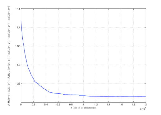
Figure 3: Reduction in the cost. At the end of the process, the final achived point is: $(H_{k}(\hat{x}^{n}_{1}),H_{k}(\hat{x}^{n}_{2}),H_{k,k_{1}}(\hat{x}^{n}_{0}|\hat{x}^{n}_{1},\hat{x}^{n}_{2}),d_{n}(x^{n},\hat{x}^{n}_{1}),d_{n}(x^{n},\hat{x}^{n}_{2}),$ $d_{n}(x^{n},\hat{x}^{n}_{0}))$ $=(0.5503,0.5586,0.0038,0.0505,0.0483,0.0036)$

VII FUTURE DIRECTIONS

Simulated annealing was recently employed in [15] to design a universal lossy compression algorithm. In this paper, we proved that in fact the same tool can be applied to devise a universal MD algorithm. We started by defining the equivalent of MD problem for ergodic processes, and defined the idea of stationary MD coding which includes three rate constraints instead of two. Extensions of these results to additional distributed coding scenarios are under current investigation.

Appendix A: Outline of the proof of Theorem 2

Outline of the proof of the first part: Let $(R_{1},R_{2},D_{1},D_{2},D_{0})\in\mathscr{R}^{\rm B}$. We need to find $(R_{11},R_{22},R_{0})$ such that $(R_{11},R_{22},R_{0},D_{1},D_{2},D_{0})\in\mathscr{R}^{\rm P}$, and (17) -(19) are satisfied.

Let $(f^{(n)},g_{1}^{(n)},g_{2}^{(n)},g_{0}^{(n)})$ be a sequence of codes at rate $(R_{1},R_{2})$ that achieves the point $(R_{1},R_{2},D_{1},D_{2},D_{0})\in\mathscr{R}^{\rm B}$. Note that for a given code, $(\hat{X}_{1}^{n},\hat{X}_{2}^{n},\hat{X}_{0}^{n})$ is a deterministic function of $X^{n}$. Using the same method used in [12], we can generate jointly stationary ergodic processes $(\hat{\mathbf{X}}_{1}^{(n)},\hat{\mathbf{X}}_{2}^{(n)},\hat{\mathbf{X}}_{0}^{(n)})$ by appropriately embedding these block codes into ergodic processes. Here the superscript $(n)$ indicates the dependence of the constructed processes on $n$. In order to code an ergodic process into another ergodic process using a block code of length $n$, we need to cover an infinite length sequence by non-overlapping blocks of length $n$ up to a set of negligible measure, and then replace each block by its reconstruction generated by the block code. The challenging part is the partitioning which should preserve the ergodicity. This can be done using R-K Theorem [13] which states that:

Theorem 5 (Rohlin-Kakutani Theorem)

Given the ergodic source X, integers $N$, $n\leq N$, and $\epsilon>0$, there exists an event $F$ (called the base) such that

1. $F,TF,\ldots,T^{N-1}F$ are disjoint,

2. $\operatorname{P}\left(\bigcup\limits_{i=0}^{N-1}T^{i}F\right)\geq 1-\epsilon$,

3. $\operatorname{P}\left(\mathcal{S}(a^{n})|F\right)=\operatorname{P}\left(\mathcal{S}(a^{n})\right)$, where $\mathcal{S}(a^{n})=\{\mathbf{x}:x^{n}=a^{n}\}$.

Since the sequence of MD block codes were assumed to achieve the point $(R_{1},R_{2},D_{1},D_{2},D_{0})$, the constructed process $(\mathbf{\hat{X}}^{(n)}_{1},\mathbf{\hat{X}}^{(n)}_{2},\mathbf{\hat{X}}^{(n)}_{0})$ satisfies the distortion constraints given in (14)-(16) at $(D_{1}+\epsilon_{n},D_{2}+\epsilon_{n},D_{0}+\epsilon_{n})$, where $\epsilon_{n}\to 0$ as $n\to\infty$. Therefore, $(\bar{H}_{n}(\mathbf{\hat{X}}^{(n)}_{1}),\bar{H}_{n}(\mathbf{\hat{X}}^{(n)}_{2}),\bar{H}_{n}(\mathbf{\hat{X}}^{(n)}_{0}|\mathbf{\hat{X}}^{(n)}_{1},\mathbf{\hat{X}}^{(n)}_{2}),D_{1}+\epsilon_{n},D_{2}+\epsilon_{n},D_{0}+\epsilon_{n})\in\mathscr{R}^{\rm P}$. Let

$$R_{11}^{(n)} :=\frac{1}{n}H(\hat{X}^{n}_{1}),$$ (A-1)

$$R_{22}^{(n)} :=\frac{1}{n}H(\hat{X}^{n}_{2}),$$ (A-2)

$$R_{0}^{(n)} :=\frac{1}{n}H(\hat{X}^{n}_{0}|\hat{X}^{n}_{1},\hat{X}^{n}_{2}),$$ (A-3)

where $\hat{X}^{n}_{i}=g_{i}^{(n)}(M_{i})$, for $i\in\{1,2\}$ and $\hat{X}^{n}_{0}=g_{0}^{(n)}(M_{1},M_{2})$. Note that since the encoder knows $(\hat{X}^{n}_{1},\hat{X}^{n}_{2},\hat{X}^{n}_{0})$, by Theorem 1, $R_{11}^{(n)}\leq R_{1}$, $R_{22}^{(n)}\leq R_{2}$, and $R_{11}^{(n)}+R_{22}^{(n)}+R_{0}^{(n)}\leq R_{1}+R_{2}$. The only remaining step is to find the relationship between $(\bar{H}_{n}(\mathbf{\hat{X}}^{(n)}_{1}),\bar{H}_{n}(\mathbf{\hat{X}}^{(n)}_{2}),\bar{H}_{n}(\mathbf{\hat{X}}^{(n)}_{0}|\mathbf{\hat{X}}^{(n)}_{1},\mathbf{\hat{X}}^{(n)}_{2}))$ and $(R_{11}^{(n)},R_{22}^{(n)},R_{0}^{(n)})$, which is not hard from the way the processes are constructed.

Outline of the proof of the second part: Let $(R_{11},R_{22},R_{0},D_{1},D_{2},D_{0})\in\mathscr{R}^{\rm P}$. This means that there exist processes $\hat{\mathbf{X}}_{1}$, $\hat{\mathbf{X}}_{2}$ and $\hat{\mathbf{X}}_{0}$ jointly stationary and ergodic with $\mathbf{X}$ which satisfy (11)-(16). Based on these processes, for block length $n$, we use the following block coding strategy: For coding sequence $X^{n}$, describe $\hat{X}_{1}^{n}$ and $\hat{X}_{2}^{n}$ losslessly to the decoders 1 and 2 using $n(\bar{H}(\hat{\mathbf{X}}_{1})+\epsilon_{n})$ and $n(\bar{H}(\hat{\mathbf{X}}_{2})+\epsilon_{n})$ bits respectively. Given $\hat{X}_{1}^{n}$ and $\hat{X}_{2}^{n}$, $n(\bar{H}(\hat{\mathbf{X}}_{0}|\hat{\mathbf{X}}_{1},\hat{\mathbf{X}}_{2})+\epsilon_{n})$ bits suffice to describe $\hat{X}_{0}^{n}$ losslessly to Decoder $0$. These bits can be divided into two parts: the first part will be included in the message $M_{1}$, and the rest in the message $M_{2}$. Decoders $1$ and $2$ just ignore these extra bits, but Decoder $0$ combines them with the two other messages to reconstruct $\hat{X}_{0}^{n}$. Since $R_{1}$ and $R_{2}$ satisfy (17)-(19), it is possible to do this.

Appendix B: Proof of Theorem 3

For an ergodic source $\mathbf{X}$, let

$$\mu(\mathbf{\boldsymbol{\gamma}},\boldsymbol{\alpha}):=$$

$$\min\limits_{\mathscr{R}^{\rm P}(\mathbf{X})}\left[\gamma_{1}R_{11}+\gamma_{2}R_{22}+\gamma_{0}R_{0}+\alpha_{1}D_{1}+\alpha_{2}D_{2}+\alpha_{0}D_{0}\right].$$ (B-1)

No coding strategy can beat $\mu(\mathbf{\boldsymbol{\gamma}},\boldsymbol{\alpha})$ on a set of non-zero probability. Therefore, the left hand side of (21) is lower bounded by its right hand side. Therefore, we only need to prove the other direction. By definition, for any $(R_{11},R_{22},R_{0},D_{1},D_{2},D_{0})\in\mathscr{R}^{\rm P}(\mathbf{X})$, there exist processes $\hat{\mathbf{X}}_{1}$, $\hat{\mathbf{X}}_{2}$ and $\hat{\mathbf{X}}_{0}$ such that (11)-(16) are satisfied. On the other hand, if $(\hat{X}_{1}^{n},\hat{X}_{2}^{n},\hat{X}_{0}^{n})$ is generated by jointly ergodic processes $(\hat{\mathbf{X}}_{1},\hat{\mathbf{X}}_{2},\hat{\mathbf{X}}_{0})$, then for $k=o(\log n)$ and $k_{1}=o(\log n)$ such that $k,k_{1}\to\infty$ as $n\to\infty$, $H_{k}(\hat{X}_{i}^{n})\to\bar{H}(\hat{\mathbf{X}}_{i})$, for $i\in\{1,2\}$, and moreover $H_{k,k_{1}}(\hat{X}_{0}^{n}|\hat{X}_{1}^{n},\hat{X}_{2}^{n})\to\bar{H}(\hat{\mathbf{X}}_{0}|\hat{\mathbf{X}}_{1},\hat{\mathbf{X}}_{2})$. This implies that

$$\limsup\min[ \gamma_{1}H_{k}(\hat{X}_{1}^{n})+\alpha_{2}d_{n}(X^{n},\hat{X}_{2}^{n})+$$

$$\gamma_{2}H_{k}(\hat{X}_{2}^{n})+\alpha_{1}d_{n}(X^{n},\hat{X}_{1}^{n})+$$

$$\gamma_{0}H_{k,k_{1}}(\hat{X}_{0}^{n}|\hat{X}_{1}^{n},\hat{X}_{2}^{n})+\alpha_{0}d_{n}(X^{n},\hat{X}_{0}^{n})]$$ (B-2)

is upper-bounded by $\mu(\mathbf{\boldsymbol{\gamma}},\boldsymbol{\alpha})+\epsilon_{n}$, where $\epsilon_{n}\to 0$. Combining these two results in the desired conclusion.

References

• [1] H. Witsenhausen, “On source networks with minimal breakdown degradation,” Bell Syst. Tech. J., vol. 59, no. 6, pp.  1083-1087, July-Aug. 1980.
• [2] J. Wolf, A. Wyner, and J. Ziv, “Source coding for multiple descriptions,” Bell Syst. Tech. J., vol. 59, no. 8, pp. 1417-1426, Oct. 1980.
• [3] L. Ozarow, “On a source coding problem with two channels and three receivers,” Bell Syst. Tech. J., vol. 59, no. 10, pp. 1909-1921, Dec. 1980.
• [4] H.S. Witsenhausen and A.D. Wyner, “Source coding for multiple descriptions II: A binary source,” Bell Lab. Tech. Rep.  TM-80-1217, Dec. 1980.
• [5] A. El Gamal and T. M. Cover, “Achievable rates for multiple descriptions,” IEEE Transactions on Information Theory, vol. 28, no. 6, pp. 851-857, Nov. 1982.
• [6] Z.  Zhang and T. Berger, “New results in binary multiple descriptions,” IEEE Trans. Inform. Theory, vol. 33, no. 4, pp. 502-521, July 1987.
• [7] R. Venkataramani, G. Kramer, and V.K. Goyal, “Multiple description coding with many channels,” IEEE Trans. Inf. Theory, vol. 49, no. 9, pp. 2106-2114, Sept. 2003.
• [8] L. Zhao, P. Cuff and H. Permuter, “Consolidating Achievable Regions of Multiple Descriptions,” submitted to IEEE Inter. Symp. on Inf. Theory, Seoul, Korea, 2009.
• [9] M. Fleming and M. Effros, “The rate distortion region for the multiple description problem,” Proc. IEEE Int. Symp. Information Theory Sorrento, Italy, Jun. 2000, p. 208.
• [10] J. Chen, C. Tian, S. Diggavi, “Multiple description coding for stationary and ergodic sources,” Proc. Data Compression Conference (DCC), pp. 73-82, 2007.
• [11] H. Cai, S. R. Kulkarni and S. Verd$\acute{u}$, “An Algorithm for Universal Lossless Compression With Side Information,” IEEE Trans. Inf. Theory, vol. 52, no. 9, Sept. 2006.
• [12] R. M. Gray, “Sliding-block source coding,” IEEE Trans. on Inform. Theory, vol. 21, pp. 357-368, July 1975.
• [13] P. C. Shields, The theory of Bernoulli shifts, Univ. of Chicago press, Chicago, 1973.
• [14] P. Br$\acute{e}$maud, Markov chains, Gibbs fields, Monte Carlo simulation, and queues, Springer, New York, 1998.
• [15] S. Jalali, T. Weissman, “Rate-Distortion via Markov Chain Monte Carlo,” submitted to IEEE Trans.  on Info. Theory. (available on arxiv at http://arxiv.org/PS$\_$cache/arxiv/pdf/0808/0808.4156v1.pdf)