Simulating the physics and mass assembly of distant galaxies out to z$\sim$6 with the E-ELT

Abstract

One of the main science goal of the future European Extremely Large Telescope will be to understand the mass assembly process in galaxies as a function of cosmic time. To this aim, a multi-object, AO-assisted integral field spectrograph will be required to map the physical and chemical properties of very distant galaxies. In this paper, we examine the ability of such an instrument to obtain spatially resolved spectroscopy of a large sample of massive ($0.1\leq M_{stellar}\leq 5\times 10^{11}M_{\odot}$) galaxies at $2\leq z<6$, selected from future large area optical-near IR surveys. We produced a set of about one thousand numerical simulations of 3D observations using reasonable assumptions about the site, telescope, and instrument, and about the physics of distant galaxies. These data-cubes were analysed as real data to produce realistic kinematic measurements of very distant galaxies. We then studied how sensible the scientific goals are to the observational (i.e., site-, telescope-, and instrument-related) and physical (i.e., galaxy-related) parameters. We specifically investigated the impact of AO performance on the science goal. We did not identify any breaking points with respect to the parameters (e.g., the telescope diameter), with the exception of the telescope thermal background, which strongly limits the performance in the highest (z$>$5) redshift bin. We find that a survey of $N_{gal}$ galaxies that fulfil the range of science goals can be achieved with a $\sim$90 nights program on the E-ELT, provided a multiplex capability $M\sim N_{gal}/8$.

1 Introduction

Over the last decade, the synergy of 8-10 meter class telescopes with HST has strongly re-invigorated the field of galaxy formation and evolution by unveiling very distant galaxies up to z$\sim$6 (e.g., Cuby et al. 2003; Rhoads et al. 2003; Bremer et al. 2004; Bouwens et al. 2006), by allowing the first determination of the global star formation history since redshift z$\sim$6 (e.g., Hopkins 2004), and by providing the first insights on the stellar mass assembly history out to z$\sim$5 (e.g., Drory et al. 2005; Pozzetti et al. 2007; Marchesini et al. 2007; Pérez-González et al. 2008). Despite these recent progresses, the outstanding question remains on how and when galaxies assembled their baryonic mass across cosmic time. The CDM standard model has provided a satisfactory scenario describing the hierarchical assembly of dark matter halos, in a bottom-up sequence which is now well-established over the whole mass structure spectrum. In contrast, little progress has been made in the physical understanding of the formation and evolution of the baryonic component because the conversion of baryons into stars is a complex, poorly understood process.

As a result, all intellectual advances in galaxy formation and evolution over the last decade have been essentially empirical, often based on phenomenological (or semi-analytical) models, which heavily rely on observations to describe, with simplistic rules, such processes as star formation efficiency, energy feedback from star formation and AGN, chemical evolution, angular momentum transfer in merging, etc. Cornerstones observations in this empirical framework are the total and stellar mass of galaxies and their physical properties, including the age and metallicities of their underlying stellar populations, dust extinction, star formation rate, and structural/morphological parameters. The study of well-established scaling relations involving a number of these physical parameters (e.g. mass-metallicity, fundamental plane, colour-magnitude, morphology-density) are essential for understanding the physical processes driving galaxy evolution. However, with the current generation of 10m-class telescopes, we have been able to construct for example the fundamental plane of early-type galaxies, or to measure the Tully-Fisher relation of late-type galaxies over a wide range of masses only at low and intermediate redshifts (z$<$1), whereas only the brightest or most massive galaxies have been accessible at z $>$ 1, and a direct measurement of masses has been almost completely out of reach at z $>$ 2. Thus, our ability to explore the evolution and origin of the aforementioned scaling relations has rapidly reached the limit of 10m-class telescopes.

Hence, most of the outstanding questions arisen from recent observational galaxy evolution studies which have pushed the 10m-class telescopes to their limits call for an Extremely Large Telescope (ELT), specifically to extend the spectroscopic limit by at least two magnitudes with near-diffraction limit angular resolution. IFU spectrographs on 8-10m class telescopes (e.g., VLT/SINFONI and Keck/Osiris) are now routinely deriving the spatially-resolved kinematics of massive (i.e., with stellar masses larger than 10${}^{10}M_{\odot}$), distant galaxies, from z$\sim$0.4 to z$\sim$3 (Flores et al. 2006; Puech et al. 2006a; Yang et al. 2008; Förster-Schreiber et al. 2006; Wright et al. 2007; Shapiro et al. 2008; Bournaud et al. 2008; Genzel et al. 2008; van Starkenburg et al. 2008; Law et al. 2009; Wright et al. 2008; Epinat et al. 2009; Förster Schreiber et al. 2009; Lemoine-Busserolle et al. 2009). Such studies have brought new and essential insights into galaxy evolution processes, such as the fraction of rotators as a function of redshift (Yang et al. 2008; Förster Schreiber et al. 2009), a better understanding of the evolution of the Tully-Fisher relation (Puech et al. 2008; Cresci et al. 2009; Puech et al. 2009), or the first glimpse into the evolution of the angular momentum (Puech et al. 2007; Bouché et al. 2007). However, several uncertainties and limitations remain, especially at the highest redshifts (i.e., z$>$1). For instance, z$\sim$2 surveys were drawn from different selection criteria (e.g., BX, BM, or BzK galaxies), and this might bias the resulting sample in a subtle and quite uncontrolled way. Besides, samples in the NIR are selected in optimal atmospheric windows, free of OH sky lines and maximising the atmospheric throughput, which intrinsically limits the redshift range and size of the resulting sample. The only way to overcome these issues is to move to telescopes with larger collecting areas.

ESO is currently developing a Phase B study for a European 42-meter telescope (Gilmozzi & Spyromilio 2008; Spyromilio et al. 2008). As part of the project development, the Design Reference Mission (DRM) aims at producing a set of observing proposals and corresponding simulated data which together provide the project with a tool to assess the extent to which the E-ELT addresses key scientific questions and assist in critical trade-off decisions. In the frame of the DRM effort, simulations of 3D high-z galaxy observations were undertaken. These observations are expected to yield direct kinematics of stars and gas in the first generation of massive galaxies (in the range 0.1 $\leq$ M $\leq$ 5$\times$10¹¹M_⊙), as well as their stellar population properties. This will allow one to derive dynamical masses, ages, metallicities, star-formation rates, dust extinction maps, to investigate the presence of disk and spheroidal components and the importance of dynamical processes (e.g. merging, in/outflows) which govern galaxy evolution. These data will also allow one to study the onset of well known scaling relations at lower redshifts, and to witness the gradual shift of star formation from the most massive galaxies in the highest density regions to less massive galaxies in the field.

To assess the science achievement of an NIR IFS on the E-ELT, as well as to better understand the interactions between the telescope, site, and instrument, we have produced an extensive set of $\sim$1000 simulations of observations of very distant galaxies. It is important to realize that if one wants to study what kind of instrument is needed to understand the galaxy mass assembly process, then one needs to explore a huge parameter space, i.e., from relaxed smooth or clumpy rotating disks to major and minor mergers, taking care of spanning all possible mass ratios, viewing angles, merger geometry and so on, which would make such a direct approach very difficult, and probably even impossible, on the practical side. Moreover, one has to recognise that our knowledge and understanding of the physics of distant galaxies is still incomplete, which necessitates to extrapolate some of their characteristics. Therefore, the simulations presented in this paper do not intend to be exhaustive in any sense. Rather, we aim at exploring this very large parameter space using reasonable assumptions and guesses. Indeed, the DRM exercise consisted in a broad exploration of the parameter space in realistic observing conditions, in order to identify possible limitations and/or breaking points, as well as interactions between the telescope, site, and instrument, which could potentially impact the telescope design.

This paper is the second of a series that explores the performances of a NIR IFS on the E-ELT. In the first paper, we presented our methodology to simulate realistic observations of distant galaxies (Puech et al. 2008b). We also produced first simulations and explored performance using a few scientifically-motivated cases. They illustrated the concept of “scale-coupling”, i.e., the relationship between the IFU pixel scale and the size of the kinematic features that need to be recovered by 3D spectroscopy in order to understand the nature of the galaxy and its substructure. In Puech et al. (2008b), we focused on the largest spatial scales, which are of particular interest because they carry most of the kinematic information useful to reveal the process underlying galaxy dynamics, i.e., whether a given galaxy is in a coherent and stable dynamical state (e.g., rotation), or, on the contrary, out of equilibrium (e.g., subsequently to a merger).

In this paper, we present an updated version of the simulation pipeline. The main improvement is related to the inclusion of thermal emissions from both the IFS and the telescope. This allowed us to explore a wider parameter space, and especially areas where observations are limited by the thermal emission rather than by the sky background (e.g., relatively faint targets in the K band). We also significantly extended the range of morpho-kinematic templates and of physical parameters (e.g., radius, mass, and velocity as a function of redshift) considered in the simulations. This paper is organised as follows. In Sect. 2, we present our methodology and the pipeline used for simulations. In Sect. 3, we detail the scientific and observational inputs used in the simulations. In Sect. 4, we present the results of the simulations, which are discussed in Sect. 5. A conclusion is drawn in Sect 6. Throughout, we adopt $H_{0}=70$ km/s/Mpc, $\Omega_{M}=0.3$, and $\Omega_{\Lambda}=0.7$, and the $AB$ magnitude system.

2 The physics and mass assembly of galaxies out to z$\sim$6 with the E-ELT

2.1 Goals of the simulations

Simulations presented in this paper focus on the sub-sample of distant emission line galaxies: due to Signal-to-Noise Ratio (SNR) limitations, absorption line galaxies at z $\gtrsim$ 1.5 will more likely be studied using integrated spectroscopy (see DRM Science Case C10-3 “ELT integrated spectroscopy of early-type galaxies at z $>$ 1”). Therefore, in the following, only emission line galaxies will be considered and for convenience, we will sometimes use the single word “galaxies” to refer to “emission line galaxies”.

Spatially-resolved kinematics of such galaxies provides a useful test-bed for 3D spectrographs, because it drives the stringent requirements on the SNR: while flux is the zero-order moment of an emission line, the velocity and velocity dispersion are derived from the position and the width of emission lines, which are their first and second moments, and higher order moments are always characterised by larger statistical uncertainties. Hence, simulations shall assess the principal scientific goal of spatially-resolved spectroscopy of distant emission line galaxies, focusing on kinematics. Different objectives can be defined depending on the level of accuracy and/or spatial scale one wants to probe; we defined the following objectives (dubbed here as “steps”), ordered by increasing complexity/difficulty:

1. Simple (3D) detection of emission line galaxies: what stellar mass can be reached at a given SNR as a function of redshift, AO system, environmental conditions, etc.?

2. Recovery of large scale motions (see, e.g., Flores et al. 2006): what are the conditions under which it is possible to recover the dynamical state of distant galaxies (e.g., relaxed rotating disks vs. non-relaxed major mergers)?

3. Recovery of Rotation Curves (RC): what are the conditions under which it is possible to recover the rotation velocity V_rot (to derive, dynamical masses or the Tully-Fisher relation, see, e.g., Puech et al. 2006a, 2008) or the whole shape of the RC (for derivation and decomposition in mass profiles, see, e.g., Blais-Ouellette et al. 2001)?

4. Recovery of the detailed kinematics: what are the conditions under which it is possible to detect internal structures in distant galaxies, like clumps in distant disks (see, e.g., Bournaud et al. 2008)?

Studying and evaluating in detail the future achievement and measurement accuracy of an NIR integral-field spectrograph on the E-ELT in these areas is beyond the scope of this paper. Moreover, in addition to the scientific limitations pointed out in the Introduction, one has to take into account the fact that technical developments (both on the telescope and instrument side) are not advanced enough to allow us to conduct such a detailed study, since several key elements are currently not fully known (e.g., the thermal contribution from the telescope, coatings, instrument design). Rather, the goal of this paper is to restrict the acceptable underlying parameter space (see below), and identify breaking points on the technical side that might strongly impact the achievable science of an IFS an the E-ELT.

However, to put this study on as realistic as possible grounds, an observational proposal was defined prior to simulations. This program was designed to provide us with an ultimate test of galaxy formation theories. It is therefore ambitious, with the goal of obtaining spatially-resolved kinematics of about one thousand of galaxies spanning a large range of cosmic time and mass. Current 3D surveys on 8-10m telescopes already allowed us to sample a significant part of the cosmic look-back time, from z=0.4 to z$\sim$3, i.e., up to $\sim$11 Gyr ago. Main 3D samples are concentrated around z$\sim$0.6 (see the IMAGES sample, Yang et al. 2008) and z$\sim$2 (see the SINS and OSIRIS samples, Förster Schreiber et al. 2009; Law et al. 2009), and it is unlikely that current or event future 3D spectrographs on 8-10m telescopes will provide us with large and representative samples beyond z$\sim$3, due to limitations in surface brightness detection, even when fed with adaptive optics. Therefore, we focused on the redshift range 2-5.6, which remains largely unexplored, with the advantage of sharing the z$\sim$2 limit with existing data. The upper limit is driven by the availability of emission lines in the NIR window, and corresponds to the [OII] emission line getting out the K band.

It is worth emphasising that such a 3D survey is by nature radically different from what is currently done at z$>$1. Because of the limited sensitivity of current 3D spectrographs, galaxies are targeted in optimal windows, where the atmospheric absorption is low. This, combined to the collection of selection criteria used at high-z to pre-select targets with known redshifts (e.g., BzK, or Lyman-break techniques) result in samples whose selection functions and representativity have been the subject of a long debate. The only way to overcome these limitations is to conduct a deep optical-NIR imaging and redshift survey with high completeness up to z$\sim$5.6, from which a 3D follow-up on the E-ELT will guarantee, without any pre-selection, the representativity of the resulting sample.

Several integral field spectrographs (IFS) are currently under study for the E-ELT. The present program is designed for a multi-object IFS, since multiplex is required to reach a significant number of targets. For example, EAGLE, the project of multi-integral field spectrograph for the E-ELT, would be a well-suited instrument for such a survey (Cuby et al. 2008; Puech et al. 2009b). However, we want to emphasise that the present paper does not intend to explore the scientific capabilities of this particular instrument, beyond the fact that it is a NIR multi-IFU spectrograph.

2.2 Simulation pipeline

The end-products of 3D spectrographs are usually data-cubes in FITS format. Hence, we have developed a simulation pipeline that produces such mock data. These simulated data are produced assuming a perfect data reduction process, whose impact has therefore been neglected (see Sect. 5.1).

Data-cubes are simulated using a backward approach of the usual analysis of 3D data. During such an analysis, each spaxel is analysed separately in order to extract from each spectrum the continuum and the first moments of emission lines. One ends up with a set of maps describing the spatial distribution of the continuum and line emissions (zeroth order moment of the emission line), as well as the gas velocity field (first order moment) and velocity dispersion map (second order moment). Such maps are routinely derived from Fabry-Perot observations of local galaxies (see, e.g, Epinat et al. 2008), or can be generated as by-products of hydro-dynamical simulations of local galaxies (e.g., Cox et al. 2006). Using simple rules and empirical relations, these maps can be rescaled (in terms of size and total flux) to provide a realistic description of distant galaxies (see Sect. 3.1). Assuming a Gaussian shape for all spectra, it is then straightforward to reconstruct a data-cube from such a set of four maps, by “reversing” the usual analysis of 3D data. This allows us to produce a data-cube at high spatial resolution, which can then be degraded at the spatial resolution (AO PSF) and sampling (IFU pixel scale) required for simulating data produced by a given 3D spectrograph. During the process, realistic sky and thermal backgrounds, as well as photon and detector noise are added. The pipeline is fully described in Puech et al. (2008b) and Puech et al. (2008c).

The simulation pipeline generates $ndit$ data-cubes with individual exposure time of $dit$, which are combined by estimating the median of each pixel to simulate several individual realistic exposures. Since we have only included random noise, it is similar to having dithered all of individual exposures and combining them after aligning them spatially and spectrally. Sky frames are evaluated separately (i.e., with a different noise realization), and then subtracted from each individual science frame, reproducing the usual procedure in both optical and NIR spectroscopy.

2.3 Overview of simulation outputs

We list here the FITS files generated by the simulation pipeline that are relevant for the present study:

• An IFU data-cube: this is the final product of the simulation, which corresponds to mock observations;

• A total background spectrum (sky continuum, OH sky lines, and total thermal background);

• A thermal background spectrum;

• An SNR data-cube, which gives the expected SNR within each pixel of the IFU data-cube. This spectroscopic SNR is derived as follows:

  $$SNR(i_{x},j_{y},k_{\lambda})=\frac{O(i_{x},j_{y},k_{\lambda})*\sqrt{ndit}}{\sqrt{O(i_{x},j_{y},k_{\lambda})+S(i_{x},j_{y},k_{\lambda})+ron^{2}+dark}},$$

  where $O(i_{x},j_{y},k_{\lambda})$ and $S(i_{x},j_{y},\lambda)$ are respectively the object and sky flux per $dit$ (after accounting for atmospheric transmission) in the spatial position $(i_{x},j_{y})$ of the data-cube (in pixels), and at the spectral position $k_{\lambda}$ along the wavelength axis (in pixels). In the following, the “maximal SNR in the emission line in the pixel $(i_{x},j_{y})$” refers to MAX${}_{k_{\lambda}}$[$SNR(i_{x},j_{y},k_{\lambda})$], and the “spatial-mean SNR” refers to the average of this quantity over the intrinsic galaxy diameter, i.e., the diameter of the galaxy irrespective of what parts of the galaxy are detected.

For each simulation, the main parameters are recorded in the headers of the corresponding FITS files.

The simulated IFU data-cubes are then analysed using an automatic data analysis pipeline similar to those generally used to analyse data of high redshift galaxies. During this process, each spatial pixel of the simulated data-cube is fitted with a Gaussian in wavelength, whose position and width correspond respectively to the velocity and velocity dispersion of the gas in this spatial pixel. Only pixels with a kinematic signal to noise ratio $SNR_{kin}$ of at least three (see definition below) were considered to limit uncertainties. A more detailed description of the process can be found in Puech et al. (2008b) and Puech et al. (2008c). The analysis pipeline produces the following FITS files:

• An emission line flux map;

• A velocity field;

• A velocity dispersion map;

• A map of the kinematic $SNR_{kin}$, which is defined as the total flux in the emission line divided by the noise on the continuum $\sigma_{continuum}$ and $\sqrt{N}_{pix}$, the number of pixels within the emission line;

• A map of the maximal $SNR$, i.e., the $SNR$ at the peak of the emission line within each spaxel of the simulated IFU data-cube. A spatial-mean value is written down into the header (see above).

2.4 Methodology for simulations

All input parameters can be separated into two broad categories, namely the “physical” parameter space, which includes all parameters defining the distant galaxy (i.e., redshift $z$, galaxy diameter, continuum AB magnitude $m_{AB}$, rest-frame emission line equivalent width $EW_{0}$, velocity gradient, and morpho-kinematic type), and the “observational” parameter space, which includes the telescope (primary mirror M1 and secondary mirror M2 diameters, temperature $T_{tel}$, and emissivity $\epsilon_{tel}$), the instrument (spectral resolution $R$, IFU pixel size $\Delta_{pix}$, detector integration time $dit$, number of exposures $ndit$, temperatures $T_{instr}$ and emissivities $\epsilon_{instr}$, AO correction, and global transmission t_transm), and the site (seeing, $C_{n}^{2}$ profile, outer scale of the turbulence $L_{0}$, sky brightness and atmospheric transmission).

Given the very large number of parameters to be investigated, as well as the very large range of values to be explored, it is useful to define a “reference case”, around which the parameter space can be explored and compared with. As such a reference case, we adopted an M_∗ galaxy at z=4 observed using MOAO (Multi-Object Adaptive Optics, see Sect. 3.2) with a median seeing of 0.8 arcsec. At this redshift, the [OII] emission line is observed in the H-band, where the influence of the thermal background is minimised in comparison with the K-band. This makes this reference case as independent as possible of the telescope design (e.g., number of mirrors), environmental conditions (site selection), and instrument characteristics (e.g., number of warm mirrors), which are not all fully known at present.

This reference case will be used to assess separately the influence of:

• the AO correction for a given set of other observational and physical parameters;

• the observational parameters for a given set of physical parameters and AO correction;

• the physical parameters for a given set of observational parameters (AO correction included).

2.5 Metrics and figures of merit

To decide whether or not the scientific goals have been met, we adopted a pragmatic point of view and defined as a general metric the total observation time of the survey $T_{intg}$ required to achieve the proposal goals, i.e., observe $N_{gal}$ galaxies more massive than $M_{stellar}=10^{10}M_{\odot}$ in the redshift range 2-5.6. A high number of galaxies ($N_{gal}\gtrsim$100) is required to allows us to derive statistics over the morpho-kinematic types of galaxies in several redshift and stellar mass bins (see Sect. 4.6). We require $T_{intg}\leq 100$ nights, which roughly corresponds to the total time allocated at ESO to Large Programs per VLT per year (i.e., 30% of the available time). Therefore, such a survey could reasonably be implemented as a several years effort. Finally, this total time should correspond to SNR levels that guarantee to reach at least step (ii) for most of galaxies in the survey, and step (iv) (see Sect. 2.1) for a more limited sub-sample (to be defined by simulations).

From a more practical point of view, such a survey will be faced with the difficulty that future targets will have to be drawn from a larger parent sample because of selection constraints on, e.g., avoidance of OH sky lines, which reduces the availability of redshift windows at a 30-40% level in H-band (see Puech et al. 2008b). Other technical constrains might be related to, e.g., the design of instrument setups in terms of spectral bandwidth. However, the current development of EAGLE, the project of multi-integral field spectrograph for the E-ELT, considers the capability of obtaining the equivalent of large-band filters in terms of spectral bandwidth in a single observational shoot (Cuby et al. 2008). Finally, the construction of this parent sample will require substantial observing time from current or future facilities (e.g., VLT/HAWK-I, JWST/NIRCAM, VISTA). Given that the target density at z$\sim$4 is of the order of one per arcmin² (down to $I_{AB}$=25, see Steidel et al. 1999, 2003, defining a parent sample of, say, one thousand of galaxies will require deep imaging in the NIR over several square-degrees. This will be further discussed in Sect. 5.

2.6 Test case

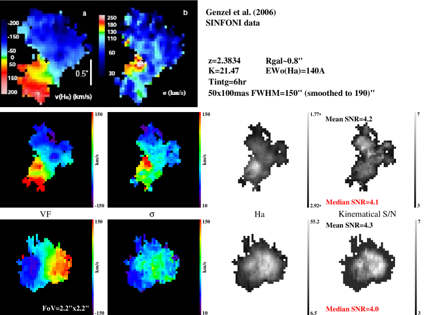
Figure 1: Comparison of SINFONI data with simulations of a rotating disk (UGC5253 template, see Sect. 3.1) using the same set of observational and physical parameters (see text). First panel: SINFONI observations of a z$\sim$2.4 galaxy (left: velocity field; right: velocity dispersion map), reproduced from Genzel et al. (2006). Second panel: analysis of the reduced SINFONI data-cube (courtesy of N. Förster-Schreiber) using our own automatic analysis pipeline (see Sect. 2.4). From left to right: velocity field, velocity dispersion map, H$\alpha$ map, and $SNR_{kin}$ map. Third panel: simulations of a rotating disk using the observational and physical parameters corresponding to the real SINFONI observations. The median $SNR_{kin}$ is found to be very similar in both cases.

We conducted a special first run to compare the results of the simulation pipeline with real 3D observations on the VLT of a galaxy at z$\sim$2.4 observed by Genzel et al. (2006) using SINFONI. The goal of this run is to use input parameters corresponding to a real observed case and assess whether or not the simulation pipeline is able to produce a data-cube with the same quality, quantified using the median $SNR_{kin}$ (see definition in Sect. 2.3). For the z$\sim$2.4 galaxy observed with SINFONI, the corresponding input parameters are: galaxy diameter of 0.8 arcsec, K=21.47, EW₀(H$\alpha$)=140Å, integration time T_intg=6 hr, pixel size of 50$\times$100 mas², PSF with FWHM=150 milli-arcsec (mas), temperature of the telescope and instrument of 287K (VLT), emissivity of the telescope of 6% (Cassegrain focus), emissivity of SINFONI of 15%. We took care of mimicking the SINFONI data reduction procedure by interpolating pixels from the physical 50$\times$100 mas² spatial scale down to the 50$\times$50 mas² final scale, and smoothing the data-cube to a resolution of 190 mas (Genzel et al. 2006) . The results of this validation run are shown in Fig. 1 and demonstrate that, given a complete set of observational and physical parameters, simulations can produce data-cubes quantitatively similar to real observations. Moreover, the similarity between the observed velocity field and velocity dispersion map (see first panel in Fig. 1) and those produced by the automatic analysis pipeline (see second panel) shows that the automatic analysis pipeline can be used safely and does not add too much uncertainty on the derived kinematics compared to a more careful visual examination and fitting of the data-cube.

3 Simulations

3.1 Scientific inputs

Scientific inputs are needed in order to (1) provide the simulation pipeline with morpho-kinematic templates and (2) re-scale these templates as a function of realistic distant galaxy sizes, fluxes, and velocity gradients. A global flowchart of the rescaling procedure is shown in Fig. 2, while specific details are given below.

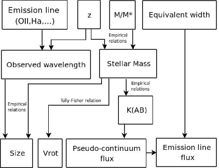
Figure 2: Schematic illustration of the method used to re-scale the morpho-kinematic templates in order to make them match the size and flux of distant galaxies. Also, the velocity dispersion (not shown here) can be rescaled using a multiplicative value.

Morpho-kinematic templates: Table 1 summarises the main properties of the high resolution templates used for the simulations, which are shown in Fig. 3 and 4. These templates were obtained from both real observations (Fabry-Perot interferometry of local galaxies, see Epinat et al. 2008 and Fuentes-Carrera et al. 2004), and hydro-dynamical simulations of galaxies (see Cox et al. 2006 and Bournaud et al. 2008).

Name	Morphological type	$inc$ (deg)	$M_{B}$ or $M_{stellar}$	$z$	Comments	Reference
UGC5253	Sab	40	-20.8	0.00441	Rotating disk	Garrido et al. (2002)
UGC6778	SABc	30	-20.6	0.003226	Rotating disk	Garrido et al. (2002)
UGC7278	Im	44	-17.1	0.00097	No rotation	Garrido et al. (2004)
UGC7592	IBm	64	-17.8	0.00069	No rotation	Garrido et al. (2004)
ARP271	SAc-SBc	59/32	-20.6/-21.2	0.0087	Merging pair	Fuentes-Carrera et al. (2004)
Major merger	Sbc-Sbc	69	5$\times$10${}^{10}M_{\odot}$	0.0	Simulation	Cox et al. (2006)
Clumpy Disks	—	50	3$\times$10${}^{10}M_{\odot}$	1.0	Simulations	Bournaud et al. (2008)

Table 1: Main properties of the morpho-kinematic templates used for the simulations. The first five templates are real observations, while the two last are hydro-dynamical simulations. From left to right: Name, morphological type, morphological inclination, absolute B-band magnitude or stellar mass for simulations, redshift, and comments.

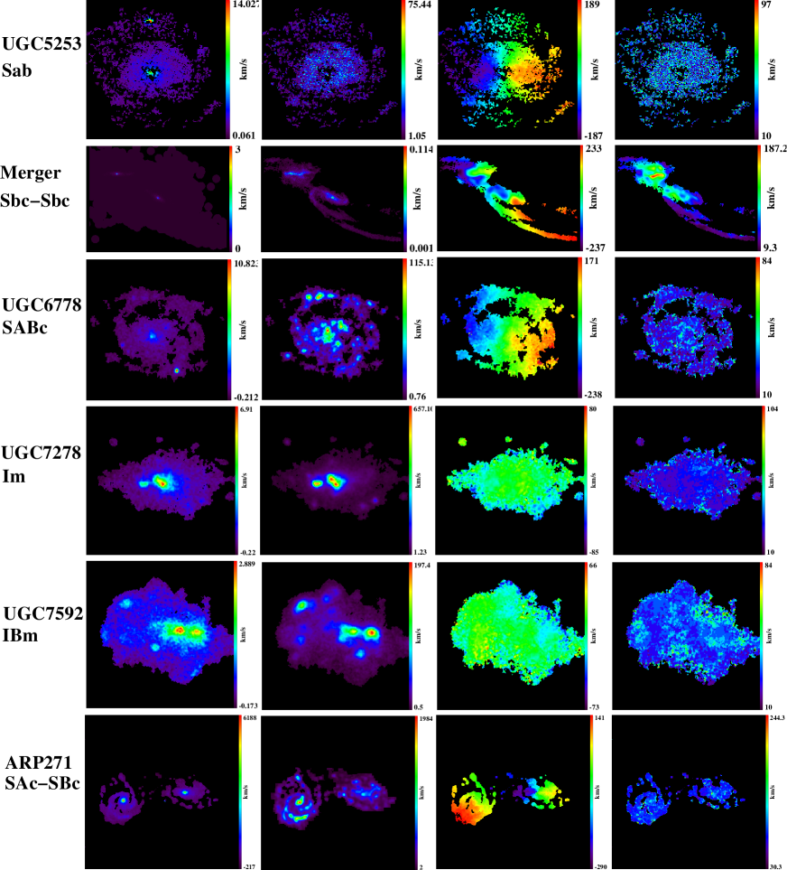
Figure 3: Morpho-kinematic templates used for the simulations. From left to right: continuum map, emission line map, gas velocity field, and gas velocity dispersion map. For the major merger simulation, the first two maps are the stellar surface density and the gas surface density maps (see Tab. 1 for details). Spatial scales are in arbitrary units since the templates are rescaled in terms of distant galaxy sizes (see text).

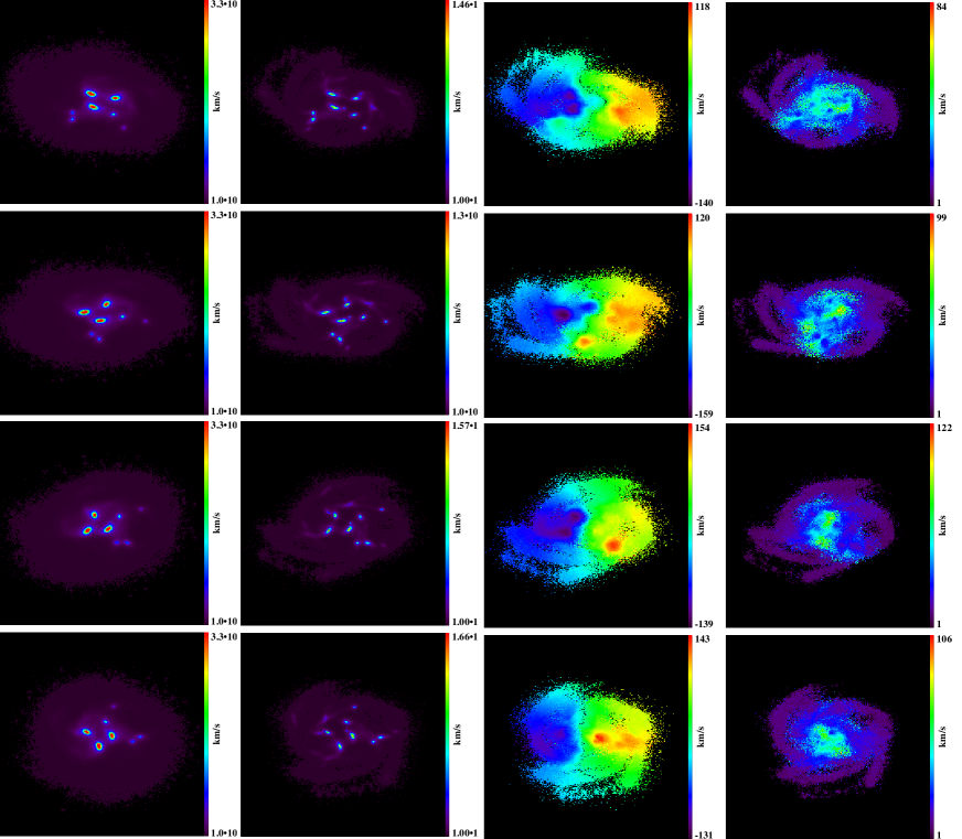
Figure 4: Morpho-kinematic templates from simulations of clumpy disks viewed from different azimuthal angles (from top to bottom: 0, 45, 90, and 135 deg). From left to right: stellar surface density map, gas surface density map, gas velocity field, and gas velocity dispersion map (see Tab. 1 for details). Spatial scales are in arbitrary units since the templates are rescaled in terms of distant galaxy sizes (see text).

Redshift: Given the objective of the present study (see introduction and Sect. 2.1), and as a compromise between the number of redshift and mass bins at constant total number of targets, three redshifts were considered for simulations. Table 2 summarises these redshifts with the corresponding targeted emission line: we chose z=2 (look-back time of 10 Gyr), z=4 (look-back time of 12 Gyr), and z=5.6 (look-back time of 12.6 Gyr), which samples well look-back times above z=2. As stated in Sect. 2.3, this choice was not driven by any consideration of optimal atmospheric transmission, but purely from scientific grounds. The impact of this selection will be discussed in Sect. 5.1.2.

For simplicity, the [OII] emission line was assumed to be a single line centred at 3727Å; this allows us to avoid introducing an additional parameter, i.e., the line ratio between the lines of the doublet, which depends mostly on the electron density in the medium (e.g., Puech et al. 2006a). This does not influence the integrated SNR over the emission line but leads to overestimate the maximal spectroscopic SNR in the emission line. The impact of this assumption will be investigated in Sect. 5.1.1. Note that the highest redshift considered (z=5.6) corresponds to the limit above which [OII] gets redshifted out of the K-band.

Stellar mass and flux: We used the MUSIC compilation of public spectro-photometric data in the GOODS field (Grazian et al. 2006) to derive empirical relations between redshift, observed K-band magnitude, and stellar-mass $M_{stellar}$ (see Fig. 5). The latter quantity was expressed as a fraction of the characteristic stellar-mass $M_{*}(z)$ at a given redshift, which describes the knee of the Galaxy Stellar Mass Function (GSMF) at this redshift, according to a Schechter function. In other words, at a given $z$, galaxies with stellar mass $M_{stellar}=M_{*}(z)$ are those which contribute the most to the stellar mass density at this redshift. Table 2 gives the corresponding stellar masses in the simulations as a function of redshift. The pseudo-continuum flux around the emission line is derived directly from the K-band magnitude. To avoid any additional parameter, we did not apply any “colour” correction between the rest-frame wavelength of the emission line (e.g., 0.3727 $\mu$m for [OII]) and that of the K-band (e.g., 0.44 $\mu$m at z=4). Such an assumption is consistent with Spectral Energy Distributions (SED) of galaxies with a morphological type latter than Sa within a factor two in flux (see, e.g., Kinney et al. 1996). As a reference case, we adopted a z=4, $M_{*}$ galaxy (see Sect. 2.4).

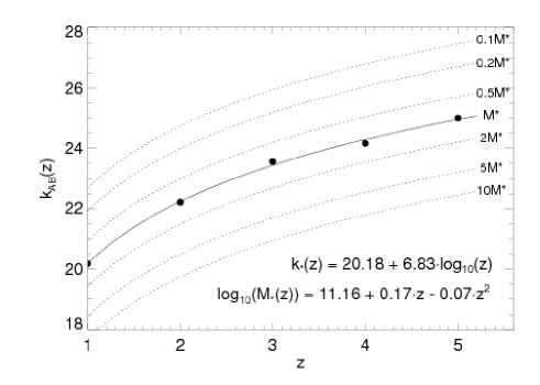
Figure 5: Empirical relations between the observed K-band magnitude and redshift used to re-scale the morpho-kinematic templates to make them match the continuum flux of distant galaxies at the corresponding stellar-mass. Black points were derived from fitting the luminosity function and mass function of galaxies in the MUSIC survey (see text). The variation of M$*$ with redshift, i.e., the knee of the GSMF, is given by the formula on the bottom. The upper formula gives the empirical evolution of the K-band magnitude of an $M_{*}$ galaxy as a function of redshift. At a given $z$, one finds that $K_{AB}=20.18+6.83\log{z}-2.5\log{M_{*}/M_{\odot}}$.

z	Look-back time (Gyr)	Emission line	Observed broad-band	Quantity	0.1$M_{*}$	0.5$M_{*}$	1.0$M_{*}$	5.0$M_{*}$	10.0$M_{*}$
2.0	10	H$\alpha~{}\lambda$6563Å	K	$log{(M_{stellar}/M_{\odot})}$	10.2	10.9	11.2	11.9	12.2
				$K_{AB}$	24.7	23.0	22.2	20.5	19.7
				$\Delta V$ (km/s)	160	210	260	350	430
				Size (arcsec)	0.68	1.19	1.52	2.67	3.40
4.0	12.0	[OII]$\lambda$3727Å	H	$log{(M_{stellar}/M_{\odot})}$	9.7	10.4	10.7	11.4	11.7
				$K_{AB}$	26.8	25.1	24.3	22.6	21.8
				$\Delta V$ (km/s)	130	180	200	300	330
				Size (arcsec)	0.33	0.59	0.75	1.3	1.7
5.6	12.6	[OII]$\lambda$3727Å	K	$log{(M_{stellar}/M_{\odot})}$	8.9	9.6	9.9	10.6	10.9
				$K_{AB}$	27.8	26.0	25.3	23.5	22.8
				$\Delta V$ (km/s)	90	110	140	200	240
				Size (arcsec)	0.28	0.50	0.63	1.11	1.41

Table 2: Redshifts (and look-back times) considered for simulations, with the corresponding emission line targeted, and the broad-band filter within which the redshifted emission line falls. On the right side: Stellar mass, K-band magnitude, velocity gradient, and size (defined as four times the half-light radius) of the simulated galaxies as a function of redshift.

Rest-frame emission line equivalent width: We assumed EW₀([OII])=30Å, which is an extrapolation of the mean value found at z=1 (Hammer et al. 1997). This parameter does not influence the emission line flux distribution of the galaxy but is used to set its total integrated value (see Puech et al. 2008b).

Size: We used empirical relations between redshift and half-light radius from the literature. To mitigate the impact of the different sample selection criteria used at high redshift, we average the different values found in the literature (Bouwens et al. 2004; Ferguson et al. 2004; Dahlen et al. 2007). The resulting “mean” half-light radius was then k-corrected using the empirical relation of Barden et al. (2005), and re-scaled to the assumed stellar-mass using the local scaling between the K-band luminosity (used as a proxy for stellar mass) and size reported by Courteau et al. (2007), i.e., $R_{half}\propto L_{K}^{0.35}$. The total size (diameter) was assumed to be four times the half-light radius. Note that in the case of a exponential thin disk of scale-length $R_{d}$, $R_{25}=3.2R_{d}$ and $R_{half}=1.68R_{d}$, which approximately leads to $R_{25}\sim 2R_{half}$. The diameters (in arcsec) used in the simulations are given in Tab. 2.

Velocity gradient amplitude: The velocity amplitude of the velocity field was rescaled using the local stellar-mass Tully-Fisher relation, following Hammer et al. (2007) (see Tab. 2). Note that strictly speaking, this procedure is quantitatively correct only if applied to rotating disk morpho-kinematic templates.

3.2 Observational inputs

Site and sky background: A Paranal-like site is assumed with T_site=280K. Atmospheric absorption is modelled following a Paranal-like site, although at a lower spectral resolution than the official current model (see bottom panel on Fig. 6). Sky emission (continuum and OH lines) was accounted for using a model from Mauna Kea, which has the advantage of also including zodiacal emission, thermal emission from the atmosphere, and an average amount of moonlight. This Mauna Kea model is two times fainter in H-band than a Paranal-like site (see upper panel on Fig. 6). The influence of the sky background will be discussed in Sect. 5.2.

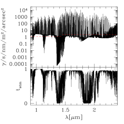
Figure 6: Atmospheric model used for the simulations. Upper panel: sky emission spectrum from the Gemini ETC (see text). The dashed-red line is the official DRM model, which is two times brighter in H band. Bottom panel: Atmospheric model from the VLT ETC.

Telescope model: We followed the official 42 meter E-ELT 5-mirror design. Its thermal background was modelled using a gray body, and assuming an emissivity of 5% (Ag+Al coating). We neglected the central aperture, as it is not included in the modelling of the PSFs (see below). The collecting area of the telescope is therefore 8% larger that the official baseline. This will be further discussed in Sect. 5.1.1.

Instrument model: We assumed a reference pixel size of 50 mas, and a reference spectral power of resolution of R=5000, as a compromise between our desire to minimise the impact of the OH sky lines and not wanting to over-resolve the line by a large factor. The instrument thermal background was modelled using two gray bodies, following a preliminary study of the thermal background of EAGLE (Laporte et al. 2008). The first one models the effect of the Target Acquisition System, and assumes a temperature of 240K and an emissivity of 15%. The second one models the effect of the spectrograph, and assumes a temperature of 150K and an emissivity of 69%. The instrument background represents less than 10% of the telescope background in both the H and K bands (see Fig. 7), in agreement with the official requirements for EAGLE, which specify that “the instrument thermal background at the detector shall be less than 50% of that from the telescope” (goal=10%). As we will see below, the total background is dominated by the thermal contribution of the telescope in the K band, and by the sky background in the H band. Therefore, we did not explore variations in the thermal contributions from the instrument, which is never the dominant source of background.

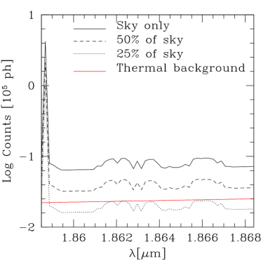
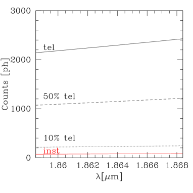
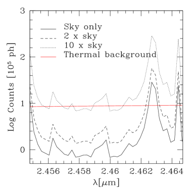
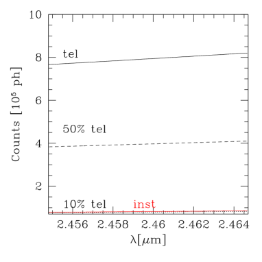
Figure 7: Contributions to the total background in the simulations, at z=4 (upper panel) and z=5.6 (bottom panel). Left column: comparisons between the sky contribution (continuum and OH sky lines, in black) and the total thermal background (telescope and instrument, in red). Right column: comparison between the telescope (black) and instrument (red) contributions to the total thermal background.

Detector model and exposure time: We rely on the description of a cooled Rockwell HAWAII-2RG IR array working at $\sim$80K, as described by Finger et al. (2006), with a read-out-noise ($RON$) of 2.3 e/pix and a dark current of 0.01 e/s/pix. Its thermal background, bias, and saturation threshold were neglected. Because observations of distant galaxies in the NIR are generally not limited by the detector noise, we did not explore parameters that have a non-negligible influence only in such a regime, i.e., variations of the individual frame exposure time $dit$, and detector characteristics ($dark$ and $RON$). In practice, we chose $dit$=3600s to speed up the simulations while keeping a reasonable number of individual exposures, although realistic exposures will be much shorter because of sky variations and saturation of the detector. We assumed a reference case exposure time of T${}_{intg}=dit\times ndit$=24 hours, i.e., $ndit$=24.

Global throughput: We assumed a global throughput t_transm=20%, detector QE included. The official DRM baseline assumes a transmission of 90-95% for the 5 mirror design telescope and a QE of 90%. The official requirements for EAGLE, specifies a throughput of at least 35%, including the detector QE. Therefore, according to the baseline, the global throughput should be 31%, which is larger that our assumption. This will be further discussed in Sect. 5.1.1. The integrated number of photons reaching the detector is a degenerated function of some parameters which have no impact on the spatial or spectral resolution, i.e., $T_{intg}$, $t_{transm}$, $EW_{0}$, and $D$. Therefore, we chose not to explore variations in global transmission, which can be directly derived by analogy with variations of associated degenerated parameters.

PSF model: The coupling between the AO system and the 3D spectrograph is captured through the AO system PSF. Therefore, it is a crucial element that needs to be carefully simulated, and cannot be approximated by, e.g., a simple Gaussian. Given the multiplex requirements for the present science case, only GLAO (Rigaut 2002) and MOAO (Assémat et al. 2007) have been considered. All PSFs include the effect of telescope aperture, but neglect the effects of the central obscuration and spiders. They were generated at the central wavelength of the corresponding filter (e.g., 1.65 microns for the H band), and the difference between this wavelength and the actual wavelength where the emission line is observed (e.g., 1.86 $\mu$m for [OII] redshifted at z=4) was neglected.

GLAO PSFs were taken from the official DRM ftp depository. These PSFs were generated by M. Le Louarn at ESO using an end-to-end code and the official DRM baseline assumptions (v1). Of note, these PSFs correspond to a total integration time of 4 seconds and therefore include non-negligible speckle noise.

MOAO PSFs were simulated using an analytical code (calibrated against an end-to-end code) by B. Neichel (GEPI-Obs. de Paris/ONERA) and T. Fusco (ONERA), which has the advantage of producing PSFs free of speckle noise, i.e., more representative of long-exposure PSFs (Neichel et al. 2008). Briefly, we used assumptions as close as possible to the assumptions used for GLAO PSF modelling: the pitch (inter-actuator distance) was assumed to be 0.5m ($\sim$84$\times$84 actuators in the pupil plane), with a reference seeing of 0.8 arcsec and an outer-scale of the turbulence $L_{0}$=25m; the same 10 turbulent layer $C_{n}^{2}$ profile that the one used for GLAO PSFs was considered. The wavefront was measured using three guide stars (assumed to be natural guide stars, i.e., specific issues related to laser guide stars like, e.g., the cone effect, were neglected), located on a equilateral triangle asterism.

In order to sample different performances for the MOAO and GLAO systems, different asterism sizes were considered. The PSFs were systematically estimated on-axis. A detailed analysis of the coupling between the MOAO and 3D spectroscopy can be found in Puech et al. (2008b). Of interest here is that in most cases, the coupling between the MOAO system and the IFU pixel scale is such that the spatial resolution is set by the latter because the PSF FWHM is smaller than twice the IFU pixel scale. Improving the MOAO correction further does not provide any gain in spatial resolution but still improves the Ensquared Energy (EE) in a spatial element of resolution (i.e., the fraction of light entering a spatial element of resolution), hence the SNR. This justifies the usual choice of characterising the EE in an aperture equal to twice the pixel size (see Puech et al. 2008b for details). The characteristics of the different PSFs used in this study are listed in Tab. 3. A detailed study of MOAO PSF shapes can be found in Neichel et al. (2008).

GLAO FoV(’)	EE in 100 mas	MOAO FoV(’)	EE in 100 mas
1	15.0	0	63.6
2	12.5	0.3	56.1
5	8.2	0.5	45.6
10	6.0	1.0	33.7
15	5.3	2.0	27.2
		3.0	24.1
		4.0	23.1
		5.0	22.7

Table 3: Sets of GLAO and MOAO PSFs generated for the simulations. The asterism size (dubbed “FoV”, i.e., the position of guide stars) is varied in order to produce a range of EE sampling typical corrections. All values were measured in the H-band with a seeing of 0.8 arcsec.

We chose reference PSFs for both AO systems as close as possible of the middle of their range of EE performances: the H-band MOAO reference PSF has EE=45.6% (in 100 mas), while the H-band GLAO reference PSF has EE=8.2% (in 100 mas). Unless stated otherwise, these two PSFs are those used in the simulations.

3.3 Simulation runs

Unless stated otherwise, parameters are by default set to their reference values as described above.

Influence of AO correction: We explore the influence of the AO correction by increasing the EE in a given aperture as described in Sect. 3.2 (see Tab. 3), for two types of AO systems, i.e., GLAO and MOAO. Simulations were done for all the morpho-kinematic templates in the MOAO case, and for the two UGC5253 and Major merger templates in the GLAO case.

Influence of observational and physical parameters: Simulations were performed for five distinct stellar masses, as described in Tab. 2, and in two different runs, as described in Tab. 4.

The simulations listed in Tabs. 2, 3, and 4 correspond to a total of about 760 individual runs.

RUN #1						RUN #2
$z$	$\Delta_{pix}$	Morpho-kin.	$EW_{0}$	$R$	$D$	$z$	$T_{intg}$	$\Delta_{pix}$	AO	Morpho-kin.	Seeing
	(mas)	Template	(Å)		(m)		(hr)	(mas)	correction	Template	(arcsec)
4	25	UGC5253-Major merger	30	5000	42	2	8	50	MOAO	ALL	0.8
	50	UGC5253-Major merger	30	5000	42		24	50	GLAO	ALL	0.8
	50	UGC5253-Major merger	15	5000	42				MOAO	ALL	0.8-0.95
	50	UGC5253-Major merger	30	10000	42	4	8	50	MOAO	ALL	0.8
	50	UGC5253-Major merger	30	2500	42		24	50	GLAO	ALL	0.8
	75	UGC5253-Major merger	30	5000	42				MOAO	ALL	0.8-0.95
	50	UGC5253-Major merger	30	5000	30	5.6	8	50	MOAO	ALL	0.8
							24	50	GLAO	ALL	0.8
									MOAO	ALL	0.8-0.95

Table 4: Observational and physical parameters investigated in the first and second run of simulations. All other parameters are set to their reference values as described in Sect. 3.

4 Results of Simulations

4.1 Influence of AO correction

The spatial-mean SNR obtained for the reference case (H band) as a function of Ensquared Energy in a 100 mas aperture (i.e., twice the reference pixel size, see above) is plotted in Fig. 8. For comparison, we also plotted results using the major merger template. This figure shows that, all simulations approximately fall along the same curve, independently of the AO type, although different codes (end-to-end vs. analytical) were used (see Sect. 3.2). This means that, considering a given morpho-kinematic template, all the different PSFs can be safely compared. For comparison to the GLAO and MAO PSFs described in Sect. 3.2, we have added MCAO PSFs (with 3DMs and asterisms of 0.5 and 5 arcmin and corrections derived at 0, 0.5,2, and 2.5 arcmin away from the centre of the FoV) and LTAO PSFs (FoV of 45 arcsec, on axis). Details about how these PSFs were generated can be found in Neichel et al. (2008b). The PSFs picked up as representative performances of the GLAO and MOAO modes (see Sect. 3.2) have been indicated by red arrows. In the H band, they can be considered as well representative of the AO performance within a range of $\sim\pm$2 in SNR for MOAO, and $\sim\pm$3 for GLAO. A systematic study of the impact of EE on the kinematics of distant galaxies using MOAO can be found in Puech et al. (2008b). Of interest here is that the reference MOAO PSF, with an EE of 45.6% in an aperture of 100 mas is above the minimal requirements derived in this study.

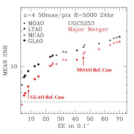
Figure 8: Spatial mean SNR obtained for the reference case (H band) as a function of Ensquared Energy in a 100mas aperture for different type of AO systems. The black points correspond to a rotating disk template, while red points correspond to a major merger template. The left most symbols represent the seeing-limited case. The GLAO and MOAO Reference Cases (see Sect. 3.2) are indicated by red arrows.

4.2 DRM Steps

In the rest of this section, we investigate the impact of the instrument, site, and telescope, on the scientific capabilities of the E-ELT equipped with a NIR-IFS in each of the DRM goals/steps as defined in Sect. 2.1.

4.2.1 DRM STEP 1: 3D detection

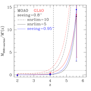
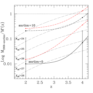
Figure 9: Left: Stellar mass limit that can be reach at a given $SNR_{min}$ as a function of redshift, AO correction, and seeing. Error-bars represent the range of mass limit obtained when considering all the morpho-kinematic templates. The vertical dashed line shows the limit above which the [OII] emission line gets redshifted into the K band. Middle: Zoom of the redshift range [2,4]. Long-dashed lines show iso-magnitude curves. For clarity, only a subset of all the curves shown in the main panel are reproduced here, and the range of mass limit is shown only for the MOAO cases with 0.8 arcsec seeing. Right: Comparison between the median emission line surface brightness of the simulated galaxies (in red; the error-bars represent the values found in the 0.1-10M$*$ range) with that from the thermal background (telescope and instrument, blue lines) and total background (thermal plus continuum and OH sky lines, black lines). For saving computation time, only narrow spectral ranges around the targeted emission lines were simulated for the three redshift cases.

We adopt a lower limit in $SNR$ of $SNR_{min}=5$ (spatial-mean SNR in the emission line, see Sect. 2.3) for the 3D detection of distant galaxies. The SNR obtained as a function of the observational parameters and mass was studied in details in Puech et al. (2008c). In this study, we found that the minimal SNR scales as follows:

$$SNR_{min}=5\times\bigg{(}\frac{T_{intg}}{24h}\bigg{)}^{0.5}\bigg{(}\frac{D}{42m}\bigg{)}\bigg{(}\frac{EW_{0}}{30\AA}\bigg{)}\bigg{(}\frac{R}{5000}\bigg{)}^{-0.5}\bigg{(}\frac{\Delta_{pix}}{50mas}\bigg{)}$$

This scaling corresponds to what is expected in a background-limited regime, and applies to all morpho-kinematic templates. As discussed in Sect. 3.2, $T_{intg}$ and the total throughput (not explicitly explored by simulations) follow the same scaling.

Figure 9 gives the stellar mass that can be reached as a function of redshift for MOAO corrections, a seeing of 0.8 arcsec, and $SNR_{min}=5$ (black line). In this plot, error-bars represent the range of stellar mass derived considering all the morpho-kinematic templates. We adopted the middle of this range as a simple estimator of the stellar mass one can reach at a given redshift under the different specific observational conditions considered in this plot (see Fig. 9). One can see that the limit in stellar mass grows exponentially with redshift:

$$\frac{M_{lim}}{M_{*}}\simeq 3.3\times 10^{-6}\exp{\bigg{(}\frac{z}{0.37}\bigg{)}},$$

which is due to the exponentially increasing contribution of the thermal background from the telescope in the NIR (see right panel in Fig. 9). Noteworthy, the mass limit evolves quite smoothly with redshift up to z$\sim$4-4.5: this means that this limit does not depend very strongly on input parameters like, e.g., seeing (see the blue curve for a 0.95 arcsec), or AO correction (see the red curve for GLAO corrections). It is not surprising that MOAO and GLAO give similar results, as the SNR considered here is a spatial-mean over the galaxy diameter at constant spatial and spectral sampling, which does not take into account differences in terms of spatial resolution (see next Section). One can adopt $SNR_{min}=10$ (instead of 5) without impacting too strongly the resulting mass limit.

It is useful to summarise Fig. 9 by deriving the redshift up to which the Galaxy Stellar Mass Function (GSMF) can be probed down to M_∗, as galaxies having such a stellar mass at a given $z$ are those contributing the most to the stellar mass density at this redshift. From Fig. 9, one can see that the GSMF can be probed down to M_∗ up to z$\sim$4, independently of the SNR limit, AO correction, and seeing conditions.

4.2.2 DRM STEP 2: Large scale motions

As detailed in Puech et al. (2008b), large scale motions carry important information about the dynamical nature of galaxies. In this section, we focus on the two extreme cases of morpho-kinematic variations found amongst the galactic zoo, which are regular rotating disks as opposed to major mergers. Indeed, because the latter are the most violent galactic events, they are expected to result in the largest morpho-kinematic amplitudes. In this section, we consider only the UGC5253 and the major merger templates to illustrate how large-scale motions can be used to distinguish between a rotating disk and a major merger using spatially-resolved kinematics on the E-ELT.

It is difficult to build a simple criterion that would allow us to assess the quality of the recovered large-scale motions, and quantify how well one can distinguish between a rotating disk and a merger in any situation. At first order, such a criterion is a function of the number of spatial element of resolutions available, and of the surface brightness detection limit. Present methods to distinguish between rotating disks and mergers are indeed limited to specific range of SNR and/or spatial resolution (see, e.g., Shapiro et al. 2008; Flores et al. 2006). Finding a method for analysing the velocity fields of distant galaxies with a large range of spatial resolution and/or SNR in a uniform way will be challenging and is far beyond the scope of this study.

Here, we adopted a simple criterion based on a threshold on the spatial-mean SNR over the intrinsic galaxy diameter, as defined in Sect. 2.3. Using MOAO, it has been suggested that a spatial-mean SNR of 5 is a minimum to recover large-scale motions and distinguish between a major merger and a rotating disk (Puech et al. 2008b). It is clear that such a criterion is generally too simplistic to allow us to distinguish between a merger and rotating disk in any possible case encountered in nature (see discussion in Puech et al. 2008b). However, it captures the two required basic dependencies on surface brightness detection (i.e., only pixels having a kinematic $SNR_{kin}$ larger than 3 are considered for the kinematic analysis, see Sect. 2.3) and on the number of available element of spatial resolutions (i.e., the spatial-mean SNR is derived over the intrinsic galaxy diameter independent of what parts are detected, see Sect. 2.3). Observations of z$\sim$0.6 galaxies using FLAMES/GIRAFFE at the VLT have demonstrated that only 3 spatial element of resolution can already allow us to distinguish between a rotating disk and more complex systems (Flores et al. 2006; Yang et al. 2008). We checked that in 98% of the simulations, a spatial-mean SNR of at least 5 corresponds to at least 3 spatial elements of resolution. Therefore, this simple criterion provides us with a useful guidance on data quality for kinematic classification, well within the scope of the present study.

In Table 5, we give the SNR obtained for a range of stellar-mass using the reference case and MOAO or GLAO corrections. According to this table, it should be feasible to distinguish between both kinds of templates down to 0.5M_∗ at z=4 using MOAO. A direct visual inspection of the simulations confirms this threshold (see Fig. 10).

Mstellar	SNR w/ MOAO	SNR w/ GLAO
(in $M_{*}(z)$)	z=4	z=4
0.1	5.45-3.85	2.58-2.53
0.5	11.09-8.80	6.41-4.40
1.0	15.54-12.76	9.12-6.75
5.0	24.84-26.07	17.89-16.46
10.0	32.24-33.27	24.21-23.46
Mstellar	SNR w/ MOAO	SNR w/ GLAO
(in $M_{*}(z)$)	z=5.6	z=5.6
0.1	0.78-0.44	0.37-0.18
0.5	1.49-1.23	0.90-0.60
1.0	2.07-1.60	1.28-0.86
5.0	3.92-3.75	2.76-2.20
10.0	5.14-5.13	3.66-3.15

Table 5: Spatial-mean SNR obtained for simulations of the reference case as a function of mass and redshift, for MOAO (upper part) and GLAO corrections (bottom part). The first value corresponds to simulations with a rotating disk template (UGC5253), while the second value corresponds to simulations with a major merger template.

Using GLAO, Table 5 suggests that the same distinction could be made down to M_∗ at z=4 (instead of 0.5M_∗ using MOAO). Since GLAO corrections smooth out many more kinematic details than MOAO, it is difficult to distinguish a major merger from a rotating disk down to the same limit in stellar mass/SNR: it is indeed difficult to visually distinguish non-circular motions in the 0.5M_∗ major merger simulations at z=4 with GLAO, as shown in Fig. 10.

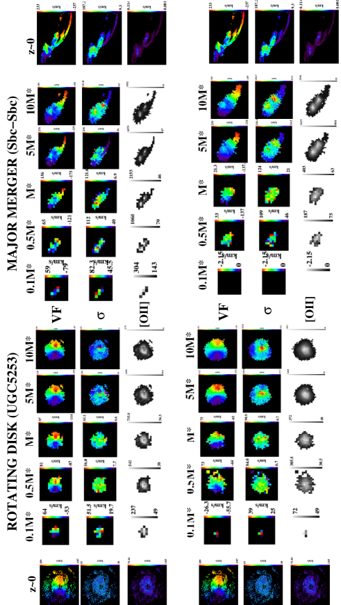
Figure 10: Results of simulations at z=4 with MOAO for the reference case (upper panels; the size of the stamps is, from left to right, 0.55, 0.95, 1.2, 2.1, and 2.7 arcsec for the rotating disk template, and 0.4, 0.7, 0.9, 1.1, and 2.0 arcsec for the major merger template) and GLAO (bottom panels). Each panel shows (from top to bottom the velocity field (first sub-panels), the velocity dispersion map (second sub-panels), and the emission line map (third sub-panels) for different stellar masses (from 0.1M_∗, first column, to 10M_∗, last column). The two panels on the left show simulations using a rotating disk template (UGC5253), while the two panels of the right show simulations for a major merger. On the leftest and rightest sides, we have reproduced the input templates shown in Fig. 3 to ease the comparison with simulations, although the spatial scales are different.

At z=5.6, the much higher background makes any distinction very difficult, and at best limits this exercise to the highest mass galaxies, as suggested by Tab. 5 and Fig. 11.

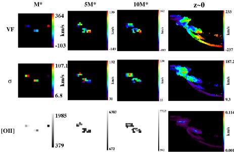
Figure 11: Results of major merger simulations at z=5.6 using MOAO. From top to bottom: velocity fields (first panel), velocity dispersion maps (second panel), and emission line maps (third panel) for different stellar masses (from 1M_∗, first column, to 10M_∗, last column). Lower mass systems are not detected. The size of the stamps is, from left to right: 0.71, 1.35, and 1.7 arcsec. On the rightest side, we have reproduced the input templates shown in Fig. 3 to ease the comparison with simulations, although the spatial scales are different.

In summary, provided a SNR of 5, these simulations suggest that it is possible, using MOAO, to recover large scale motions of galaxies and distinguish between different dynamical states at least up to z=4 and down to M_stellar=0.5M_∗. GLAO appears to provide very similar performances, although at lower spatial resolution, which would limit the recovery of the dynamical state down to $\sim$M_∗ at z=4. At higher redshift, the loss of SNR induced by the increasing contribution of the thermal background of the telescope, will limit the recovery of large-scale motions to very massive systems.

4.2.3 DRM STEP 3: Rotation Curves

In Figure 12, we show rotation curves extracted from simulations at z=2 and z=4 using the UGC5253 rotating disk template. This template has the steepest velocity curve gradient among the morpho-kinematic templates, and is therefore useful to assess at which extent which parts of the rotation curve can be recovered safely. Indeed, the central part of the rotation curve is well-known to be strongly affected by limited spatial resolution, an effect known for long as “beam smearing” by HI observers. Among the dynamical parameters fitted to derive a rotation curve from a velocity field (see, e.g., Epinat et al. 2008 for details), inclination is by far the one that carries the largest uncertainty. Indeed, there is a well known degeneracy between inclination and rotation velocity during such a fitting. Epinat et al. (2009b) have extensively studied these degeneracies as a function of beam smearing using artificially redshifted galaxies at z=1.7. These authors concluded that the best strategy is to use high-resolution broad-band imaging to derive a morphological estimate of the inclination, and use this to relax one parameter during the kinematic model fitting. We therefore did not try to fit the inclination, which was held constant during the velocity field, and focused instead on the influence of different AO modes in recovering spatial features of the rotation curve. In other words, we assumed that high-resolution imaging will be available to provide the observer with unbiased estimated of this parameter. We adopted a simple arctan rotation curve model, which is fully described by two parameters (Courteau 1997).

At z=2, only MOAO can more or less recover the rising part of the rotation curve (RC). Due to its much lower spatial resolution (FWHM_GLAO=161mas and FWHM_MOAO=11mas), GLAO induces a strong beam smearing-like effect, as in HI observations of local galaxies. Even with MOAO, the spatial sampling of the IFU (50mas/pix) limits the spatial resolution of the observations (to $\sim$0.1 arcsec) and does not allow us to recover the true shape of the RC. Compared to the best RC that one can recover at this spatial scale (see the black dashed line), MOAO and even GLAO do not induce any bias in terms of rotation velocity. However, numerical simulations will be needed to recover the true rotation velocity, as it is already the case in lower redshift kinematic studies of distant galaxies (see, e.g., Flores et al. 2006; Förster-Schreiber et al. 2006; Puech et al. 2008).

At z=4, the lack of spatial resolution will limit the study of rotation curves to super-M_∗ rotating disks, as shown in Fig. 12. At these redshifts, only MOAO will provide enough spatial resolution to limit biases in recovering the rotation velocity or the rising part of the RC.

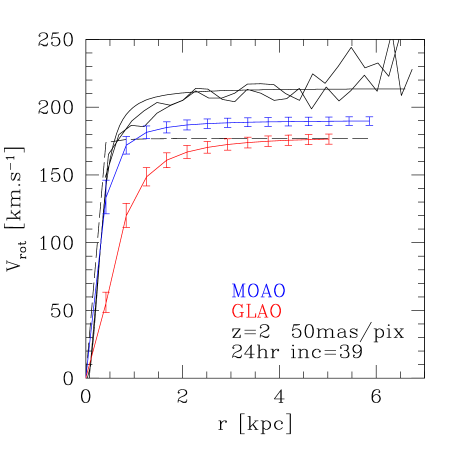
Figure 12: Rotation curve of a $z$=2, $M_{*}$ galaxy (left), and a $z$=4, 5$M_{*}$ galaxy (right). The black lines represent the original z=0 rotation curve rescaled to the size of simulated z=2 and z=4 galaxies. The rotation curve on each side of the galaxy is shown, along with an arctan fit. The rotation curve obtained using MOAO is shown in blue, while the one obtained using GLAO is shown in red. Error-bars represent only the uncertainty associated to the two parameters of the arctan function, and do not take into account uncertainties associated to other kinematic parameters like the dynamical centre or the Principle Axis. The black dashed line represent the rotation curve obtained in simulations without PSF: they correspond to the best rotation curve that one can obtain at the pixel scale of the simulations (50mas/pix).

In summary, the recovery of the whole shape of the RC will propably be limited to z$\sim$2, using MOAO. The recovery of the true rotation velocity will require numerical simulations, which is already the case in lower-z studies. At higher redshifts, such measurements will probably be limited to super-M_∗ galaxies. Using GLAO strongly degrades the shape of the recovered RC and probably prevents any accurate recovery of its true shape.

4.2.4 DRM STEP 4: Detailed kinematics

To illustrate the capability of the E-ELT in recovering the detailed kinematics of distant galaxies, we consider in this section the result of simulations with the Jeans-unstable clumpy disk templates shown in Fig. 13. Clumps can clearly be distinguished in galaxies more massive than M_∗ at z=4, using MOAO (see emission line maps). Using GLAO does not allow us to identify these clumps anymore: even in the most massive galaxy simulated, all clumps are smoothed together in the emission line map. One can still recover non-circular motions in the velocity field, but without clear morphological signature, it is difficult to identify the underlying cause of this perturbation. At higher redshift, the limited SNR does not allow us to recover such clumps anymore, even in the most massive case.

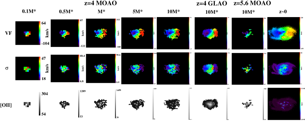
Figure 13: From left to right: Simulations of clumpy disks at z=4 using MOAO (from 0.1M_∗, first column, to 10M_∗, last column; the size of the stamps is, from left to right: 0.7, 1.25, 1.6, 2.8, 3.55 arcsec), GLAO at z=4 (10M$*$; the size of the stamp is 3.55 arcsec), and MOAO at z=5.6 (10M$*$; the size of the stamp is 3.0 arcsec). For each column, the first line shows the velocity fields, the second line the velocity dispersion maps, and the third line the emission line maps. On the rightest side, we have reproduced the input templates shown in Fig. 4 to ease the comparison with simulations, although the spatial scales are different.

In summary, these simulations suggest that it is possible to recover clumps in rotating disks down to z=4, M_∗ galaxies using MOAO. Using GLAO probably prevent any direct identification of clumps in very distant galaxies.

4.3 Compliance with figures of merit

The goal of this simulated experiment was to study a large number $N_{gal}$ of galaxies (in order to allow one to derive statistics over the morpho-kinematic types within each mass and redshift bin) at $2\leq z<6$ with $0.1\leq M_{stellar}\leq 5\times 10^{11}M_{\odot}$ in less than 100 nights. We adopt the following assumptions as a typical observational strategy for this program:

• Reference case with R=5000 and $\Delta_{pix}$=50mas (see Sect. 3);

• MOAO corrections;

• Mauna-Kea-like background, as described in Sect. 3;

• A limiting SNR of 10 (10-$\sigma$ detection);

• Overheads of 30% (i.e., overhead factor $OH$=1.3);

• The number of effective observed hours per night is assumed to be 8 hr;

• Three redshift “bins” ($z$=2, $z$=4, and $z$=5.6) and three mass “bins” per redshift bin ($\sim$0.5$M_{*}$,$\sim M_{*}$, and $\sim$5$M_{*}$), except for the $z=5.6$ case, which has only two mass bins ($\sim M_{*}$, and $\sim$5$M_{*}$), since we are interested in galaxies having $0.1\leq M_{stellar}\leq 5\times 10^{11}M_{\odot}$ and that M_∗(z=5.6)=0.8$\times$10¹⁰M_⊙. We therefore assume that the survey is divided into $N_{bins}$=8 elementary bins;

• The number of galaxies per elementary bin is assumed to be $N_{gal/bin}$. This translates into total number of galaxies in the survey of $N_{gal/bin}\times N_{bins}$.

• Within each bin of the survey, the $N_{gal/bin}$ galaxies can be observed in $N_{setups}$ setups, with $N_{setups}$=$N_{gal/bin}$/$M$ where $M$ is the multiplex advantage of the instrument, i.e., the number of galaxies that can be observed at the same time. We assume $M\geq N_{gal/bin}$, which means that all galaxies in a given bin can be observed using only one instrument setup ($N_{setup}=1$).

Under these assumptions, the corresponding integration times, in nights, needed in each elementary bin are given in Tab. 6. The great collecting power of the E-ELT is clearly reflected in the time needed to survey the redshift range 2-4, which requires only $\sim$7 nights. Regarding the z=5.6 bin, the large thermal background of the telescope (see Figs. 7 and 9) translates into very large integration times.

Tintg	0.5M∗	M∗	5M∗	Total
z=2	1.2	0.8	0.3	2.3
z=4	2.3	1.4	0.6	4.3
z=5.6	—	66.9	16.39	83.2
Total	3.5	69.1	17.2	89.8

Table 6: Integration time needed to complete the survey, in nights, assuming a multiplex $M\geq N_{gal/bin}$.

The total time of the survey, in nights, can be expressed as follows:

$$T_{survey}(n)\simeq 90\bigg{(}\frac{SNR_{lim}}{10}\bigg{)}^{2}\bigg{(}\frac{OH}{1.3}\bigg{)}\bigg{(}\frac{N_{gal}}{8M}\bigg{)}$$

As an example, if one wants to construct a 90-nights survey with a very large sample of $N_{gal}$=1000 galaxies, a multiplex factor of $M$=125 will be required. However, it is likely that the future multi-object integral field spectrograph on the E-ELT, such as EAGLE (Cuby et al. 2008), will not provide us with such a large multiplex capability. At constant $T_{survey}$, the relation between the multiplex capability $M$ and the total number of galaxies in the survey is $N_{gal}=8M$. Therefore, if one still requires such a large number of galaxies with a lower multiplex factor, e.g., $M$=25, then a total observation time of 5$\times$90=450 nights will be necessary to complete the survey. Alternatively, one can decide to reduce the number of galaxies: with $M$=25, 200 galaxies can be observed within $T_{survey}$=90n. Such a program would certainly provide a very interesting and useful first glimpse of the galaxy mass assembly process as a function of time.

In summary, with a total integration time of 90 nights, and within the assumptions listed above, it will be possible to:

• Observe $N_{gal}$ galaxies with SNR=10 in three redshift bins (2-4-5.6) and three mass bins $(0.5M_{*}$-$1.0M_{*}$-$5M_{*})$, except for the $z=5.6$ bin, which has two mass bins ($\sim M_{*}$, and $\sim$5$M_{*}$); all bins have $M$ galaxies (i.e., the multiplex gain of the instrument), which will allow one to do statistics over morpho-kinematic types;

• Recover the large-scale motions of galaxies at least up to z=4 and down to $M_{stellar}=0.5M_{*}$, i.e., of most galaxies in the survey;

• Recover the detailed kinematics of the most massive galaxies (the detection of clumps in rotating disks will be possible down to z=4, M_∗ galaxies).

5 Discussion

5.1 Limitations and accuracy of simulations

5.1.1 Observational inputs

For simplicity, we adopted several assumptions that might impact the results of the simulations in terms of SNR (see Sect. 3). First, we adopted a conservative global throughput, while proposed designed (e.g., EAGLE) predict throughput higher by a factor $\sim$55%. This would translate into an increase of the SNR by $\sim$25%, since $SNR\propto\sqrt{t_{trans}}$. Second, we have neglected the central obscuration of the E-ELT, which leads to overestimate the SNR by $\sim$8%, since $SNR\propto D$. Finally, we have assumed that the [OII] doublet in a single emission line instead of a doublet. The average [OII] line ratio is 1.4 (Flores et al. 2006), which leads to an overestimation of the maximal SNR in the emission line by a 41% at constant flux (based on the crude assumption of two resolved Gaussians), which in turn leads to overestimate the spatial-mean SNR by the same factor. All these assumptions lead to overestimate the spatial mean SNR by $\sim$24%, or, equivalently, the simulations correspond to an $EW_{0}\sim$37Å instead of 30Å, which was chosen as an extrapolation of the mean $EW_{0}$([OII]) observed at z$\sim$1 (Hammer et al. 1997). This new value is actually closer to the median $EW_{0}$([OII]) observed at z$\sim$1 (Hammer et al. 1997): such a value is as relevant as the first one, and therefore we conclude that the adopted simplifications do not impact strongly the results.

The most important limiting factors related to the observational parameter space are certainly the emissivity of the telescope, which drives the thermal emission from the telescope, which limits the detectability of high-z galaxies in the K band, and the brightness of the sky continuum between OH lines, which limits observations at lower redshift (see Sect. 4.2). As noted in Sect. 3.2, the sky continuum could indeed be two times brighter than assumed, based on a comparison between Mauna Kea and Paranal sites. This would directly impact the achieved SNR by a factor $\sqrt{2}$, e.g., a mean SNR of 10 would translates into a mean SNR of 7.1. On the other hand, an emissivity of 15% (pure Al coating) would imply a three times higher thermal background, reducing the SNR even further, by a factor $\sqrt{3}$: a mean SNR of 10 would translate into a mean SNR of 5.8. These different assumptions directly impact the achieved SNR at a given redshift and mass. For instance, this would lower the redshift up to which the GSMF can be probed down to $M_{stellar}$, from z=4.1 down to z$\sim$3.8-3.9. Therefore, while this could impact observations on a galaxy-by-galaxy basis, it would not impact them strongly in a statistical sense.

One of the current limitation of the simulations is that most of inputs are currently considered as invariant with wavelength (e.g., throughput, emissivity), because the design of the telescope and the instrument are not fully known at the moment. Simulations will need to be updated once these characteristic curves will be known. However, we expect this to be a second order effect, as characteristic curves are known to vary only very specific small windows (e.g., absorption features in optics transmission curves).

Finally, it is worth noting that we assumed a photon-starved sky subtraction: sky and science frames were simulated using a different noise realisation, which generated random errors only. This choice was driven by the fact that, in the NIR, galaxies are usually selected in redshift such that their emission lines fall in spectral windows free of OH sky lines. In this case, the sky subtraction process can reasonably well be assumed to be limited by the photon noise on the sky continuum. This assumption implies that sky subtraction is not affected by systematic errors. Further simulations related to the data reduction strategy will be required to assess the impact of such biases (affecting, e.g., measurements and/or estimation of sky frames).

5.1.2 Scientific inputs

In reality, the morpho-kinematic range of templates is significantly broader than the one used for the simulations. Because our knowledge of galaxy formation is still incomplete, the limited number of templates was chosen in order to cover a wide range of surface brightnesses. We have intentionally focused on a few representative cases, ranging from major mergers with complex morpho-kinematics to irregular galaxies with flat velocity fields, and regular rotating disks with different velocity gradients. Despite their limited number, these templates should span most interested cases.

The impact of the different surface brightness distributions can be seen in the middle panel of Fig. 9, where error-bars reflect the range of mass that can be reached at a given redshift and S/N for the 10 different morpho-kinematic templates considered in this work. We find a tendency for the most irregular surface brightness distributions to result in a largest mass limit at a given total flux. Such surface brightness distributions result in a more complex coupling between adjacent spectra in the IFS at limited spatial resolution, which in turn results in emission lines with a lower peak and larger wings compared to more regular distributions in surface brightness.

Results from high resolution imaging and spatially-resolved spectroscopy have revealed that high-z galaxies have very different properties in their morphology and kinematics, compared to local galaxies (e.g., Elmegreen & Elmegreen 2005; Förster Schreiber et al. 2009). In particular, these observations suggest that a significant fraction of high-z galaxies would be rotating clumpy disks (e.g., Genzel et al. 2008). We find that at z$\sim$2, the mass limit of clumpy disks is roughly one order of magnitude larger than more regular galaxies. Transposing this result on current 3D samples observed with 8-10m telescopes, this could explain why very distant galaxies detected by 3D spectroscopy so far, which are largely dominated by irregular surface brightness distributions (e.g., Förster Schreiber et al. 2009), systematically show very large equivalent widths in their emission lines to be detected. If a significant fraction high-z galaxies are indeed clumpy disks, then the true average SNR at a given redshift and mass might be biases toward the largest values in the range shown in Fig. 9.

Most of physical quantities used as inputs are not known to a factor better than two. We first discuss the source of uncertainty associated with the intrinsic scatter of the scaling relations used to rescale the morpho-kinematic templates in terms of flux and size. The empirical relations between stellar mass and K-band magnitude as a function of redshift have typical uncertainties of 0.3 dex (i.e., 0.75 mag, but likely more at z$\geq$4, see Sect. 3.1). This uncertainty on the stellar mass directly translates into a 0.1 dex uncertainty on $\log{R_{half}}$, using the scaling relation between stellar mass and half-light radius $R_{half}$ adopted in Sect. 3.1. This is to be compared to the intrinsic scatter of this relation (0.3 dex in $\log{R_{half}}$, see Courteau et al. 2007), to the scatter of the size versus wavelength relation (0.04 dex in $\log{R_{half}}$, see Barden et al. 2005), and to that of the size versus redshift relation ($\sim$0.06 dex in $\log{R_{half}}$, see Bouwens et al. 2004; Ferguson et al. 2004; Dahlen et al. 2007). The two dominant sources of uncertainty are clearly the redshift vs. stellar mass / K-band magnitude relation and the scatter of the stellar-mass vs. size relation, with roughly an uncertainty of a factor two in size and total flux.

Another source of uncertainty is the possible evolution of these relations with redshift. While the stellar mass vs. size relation does not appear to evolve, at least up to z$\sim$1 (Barden et al. 2005), the Tully-Fisher relation appears to evolve smoothly with redshift (a factor two in mass between z=0 and z$\sim$0.6, see Puech et al. 2008, slightly more at z$\sim$2, see Cresci et al. 2009). In this paper, we assumed no evolution of this relation: this is conservative as, at a given stellar mass, high-z rotating disks would have larger rotation velocities, which would make the associated velocity gradients easier to be detected. The scatter associated to the stellar mass Tully-Fisher Relation is $\sim$0.15 dex in $\log{M_{stellar}}$, meaning that it will not introduce significant additional uncertainty on the stellar mass / K-band magnitude compared to the stellar mass vs. size relation (see above).

Finally, one of the less constrained physical parameter is perhaps the emission line equivalent width in very distant galaxies. This parameter does not influence the flux distribution but only its total intensity. We have adopted the median value found for [OII] at z$\sim$1 (see Sect. 3.1 and 5.1.1), with an associated scatter of 15-20Å, depending on sample selection (Hammer et al. 1997). Larger values were observed at larger redshift, especially with H$\alpha$ (Erb et al. 2006). It is indeed expected that the typical equivalent widths increase with redshift, as a result of the increase of the star formation density with redshift, at least up to z$\sim$2 (Hopkins 2004). In this paper, we chose not to parametrise emission line equivalent width as a function of redshift. In practice, such a parametrisation would be largely affected by the sample selection criteria at very high-z, and the physical processes driving and affecting emission within different lines, as one has to switch from H$\alpha$ to [OII] above z$\sim$4. We therefore decided not to introduce any additional uncertain parameter and adopted the observed [OII] median value at z=1 as a conservative value. Moreover, adopting a constant value helps to disentangle the different sources of surface brightness evolution with redshift, which are only due to mass and size evolution in this study. The results given in Sect. 4.2 are to this respect conservative, especially between z$\sim$2 and 4, where observations are not strongly limited by the thermal emission from the telescope: considering an equivalent width of 100Å  in H$\alpha$, as it is often observed in z$\sim$2 galaxies (e.g., Förster Schreiber et al. 2009), instead of 30Å, would imply an increase by a factor 3 of the mean SNR (see Sect. 4.2).

We therefore conclude that simulations are internally-consistent within a factor two in all the physical quantities considered. For instance, the empirical relations between stellar mass and K-band magnitude are uncertain within a factor two, but the flux correction between the rest-frame wavelength corresponding to the K-band and that of the emission line considered is also less than a factor two (see Sect. 3.1).

Finally, in this DRM program, we assumed that targets will be selected from future deep and complete optical-NIR imaging and redshift surveys. Such surveys could potentially be done using existing facilities such as VISTA or the LSST, but will probably also benefit from the follow-up of future instruments such as JWST/NIRSPEC or ALMA. To guarantee the representativity of the sample and optimise the sampling of the look-back time axis, we did not assume any pre-selection in colour, nor do we pre-select redshifts in terms of atmospheric transmission as it is currently done on 8-10m telescopes. This allows us to take advantage of the huge collecting power of the E-ELT, and target any potential galaxy regardless of its redshift. As an alternative observational strategy, one could select more optimal redshift windows in correspondence of atmospheric windows, which would directly result in a gain of SNR and survey speed. Looking at Fig. 6, optimal windows are around 1.6 $\mu$m (which corresponds to z$\sim$3.3 using [OII]), and 2.2 $\mu$m (which corresponds to z$\sim$2.3 using H$\alpha$ or 4.9 using [OII]. Selecting galaxies in these windows would guarantee an atmospheric transmission $\sim$95% (provided that targets are selected between strong absorption features), i.e., roughly a factor two larger than the atmospheric transmission corresponding to simulations at z=2, with 44%, and at z=4, with 63%: for instance, targeting galaxies at z$\sim$2.3 instead of z=2, would result in a gain of 2.2 in SNR. Such a factor is well below the inherent uncertainty associated to the simulations (see above).

5.2 Impact of telescope design and size

The telescope is by far the dominant source of background in the K-band. Because the SNR is in a background-limited regime at z=5.6 (see Fig. 9), the telescope emission limits source detection at very high redshift. Note that in the simulations, we have used an optimistic assumption for the emissivity of the 5-mirror E-ELT design, with $\epsilon_{tel}=$5%.

MOAO provides only partial seeing corrections, therefore the resulting PSF is dominated by residual atmospheric perturbations (Assémat et al. 2007). This implies that the telescope diameter does not directly influence the spatial resolution of observations, but only the achieved SNR. The scaling relation of Sect. 4.2 shows that there is no breaking point in telescope diameter: with a smaller 30m telescope, one would need two times longer exposures to reach the same SNR.

In terms of survey speed, the E-ELT represents a huge improvement compared to existing 3D spectrograph on 8-10m telescopes. The fiducial program depicted in Sect. 4.3 will deliver 75 galaxies at z$\sim$2 covering the whole mass spectrum in only 2.3 nights. It is worth comparing this number with, e.g., the SINS survey at the VLT. Förster Schreiber et al. (2009) described this survey of 63 galaxies and gave an average integration time of 3.4 hr per galaxy (per band), which represent about 27 VLT nights in total. Note that this does not account for observing time lost because of undetected targets. The E-ELT will allow us to observe roughly the same number of galaxies, but saving more than a factor 10 in time. In addition, one should consider that SINS galaxies have typically an emission line equivalent width of $\sim$100Å, while the simulations assume 30Å. Rescaling simulations with a gain of 3 in equivalent width leads to a gain of 9 in integration time. It basically means that the SINS survey could be completed in less that one night with the E-ELT. Moreover, the E-ELT will enable a better control of the selection function: because of the limited sensitivity of current 8-10m telescopes, pre-selection in colour must be used to draw 3D distant samples beyond z$\sim$1 (see Sect. 2.1). In comparison, the E-ELT will allow us to conduct a very complete 3D follow-up of a pure mass-selected sample. Sect. 4.2.1 demonstrates that the E-ELT will allow us to draw such samples up to z$\sim$4-5. Such a limit will clearly remain out of reach of current 8-10m telescopes, except for a handful of targets.

5.3 Impact of site properties

The sky is the dominant source of background only for $z\leq 4$ observations. Note that in the simulations we have used a sky model from Mauna Kea, which is $\sim$2 times fainter in the H band that the official DRM Paranal model (see Sect. 3.2 and Fig. 6). As $SNR\propto 1/\sqrt{background}$ in such a regime, a site having two (four) times higher background than the one used in the simulations will reduce the achieved SNR from, e.g., 10 to 7 (5). The impact on high-redshift observations is therefore relatively limited (see Fig. 9).

The SNR loss between observations with a seeing of 0.8 arcsec and observations with a seeing of 0.95 arcsec is 5-15%. The strongest impact of worst seeing conditions will be to limit the capability to recover Rotation Curves and detailed kinematics of distant galaxies.

5.4 Impact of Instrument

GLAO limits the achievable SNR to lower values, compared with MOAO. As a consequence, the recovery of the large scale motions in distant galaxies using GLAO is limited to higher masses. Any further objective of the DRM will be strongly limited in using GLAO instead of MOAO (e.g., rotation curves, detailed kinematics).

Appropriate targets in the NIR are usually selected such as they have emission lines that fall in regions free of strong OH lines. This requires a minimal spectral resolution of R$\sim$3000 to resolve OH sky lines with enough accuracy. On the other hand, the highest the spectral resolution, the better the accuracy on the recovered kinematics (see Tab. 7): at least R=5000 is required if one wants to recover the velocity dispersion with no more that 50% of relative uncertainty. This value appears to be a good compromise between the desire to minimise the impact of the OH sky lines and not wanting to over-resolve the line by a large factor: the scaling relation between SNR and R (see Sect. 4.2) demonstrates the interest of having the smallest spectral resolution possible, which optimises the achieved SNR.

The choice of the IFU pixel scale drives the spatial resolution of MOAO-fed 3D spectroscopy observations, as in the range of EE provided by MOAO, the PSFs have a FWHM largely smaller than twice the pixel size. Therefore, the choice of the optimal IFU pixel scale is related to the optimal “scale-coupling” between the IFU pixel scale and the spatial scale of the physical feature that one wants to recover using this IFU (Puech et al. 2008b). This can be quantified by using the ratio between the size of this feature (here, the galaxy diameter, as one wants to recover the large-scale rotation) and the size of the IFU resolution element. 3D observations of z$\sim$0.6 galaxies with FLAMES/GIRAFFE have demonstrated that a scale-coupling of at least 3 can already provide us with useful information on large-scale motions (Flores et al. 2006), allowing us to distinguish rotating disks from other more complex systems (Puech et al. 2006a; Yang et al. 2008). Epinat et al. (2009b) showed that such a scale-coupling is enough to provide us with unbiased estimated of the PA and rotation velocity in distant galaxies. It corresponds to the minimum value necessary to ensure that each side of the galaxy is at least spatially sampled by the IFU at the Nyquist rate. Of course, there are specific situations where a finer spatial sampling is desirable in order to properly distinguish between complex systems and rotating disks (see, e.g., Epinat et al. 2009b), but using this as a guide-line provide us with a useful upper limit on the IFU spatial sampling, which is optimised for very high surface brightness detection. In the z=4 simulations, this minimal scale-coupling leads to a pixel scale of  55mas, 125 mas, and 280 mas for 0.1, 1, and 10 M* galaxies, respectively. Hence, a minimal pixel scale of 50 mas is required if one wants to be able to recover, at least in principle, large-scales motions in z=4 galaxies, and for a large range of stellar-mass.

Figure 10 shows the velocity fields, velocity dispersion maps, and emission line maps extracted from the simulations using a 50 mas pixel scale. It is clear that the lowest mass case barely provides enough spatial information to clearly distinguish between the rotating disk and the major merger. Even if the scale-coupling is in principle large enough to properly recover large-scale motions, the pixel scale limits the achieved SNR to relatively low values (see Tab. 5). If one only wants to recover large-scale motions in the most massive objects, then an IFU pixel scale of 75 mas can be used, providing more SNR at constant integration time (see Puech et al. 2008b).

Finally, we adopted 50 mas as a reference pixel scale in the simulations. This resulted from a compromise between resolving sub-kpc scales (100 mas represent 0.7 kpc at z=4) and the resulting surface brightness sensitivity. We derived the emission line flux sensitivity per pixel in the following way. We considered only simulations with 50 mas per pixel and R=5000 (the result can be easily rescaled to any other couple of spatial and spectral sampling). Then, we constructed the histogram of the emission line flux corresponding to a threshold of $SNR_{kin}$ larger than three (which defines the spaxels used for analysing the VF, see Sect. 2.1). In this histogram, we considered all simulations with integration times of 24 hr, but with different seeing, AO correction and morpho-kinematic templates, which allow us to average over a large number of different observational conditions. We found that this histogram peaks at 2$\times 10^{-20}$erg/s/cm².

In the simulations, we also explored a 25 mas pixel scale, which allowed us to bracket the EAGLE baseline with 37.5 mas. Compared to our reference case, the EAGLE baseline (R=4000 and 37.5mas/pix) would imply a 16% decrease in SNR per spatial and spectral element of sampling (see Sect. 4.2.1), and degrade the emission line flux sensitivity limit by a factor 2.2. However, the EAGLE pixel scale provides an optimal scale-coupling with distant clumps that are ubiquitous in distant galaxies (Elmegreen & Elmegreen 2005): such clumps are typically 1 kpc is diameter, therefore such a pixel scale would provide us with a scale-coupling of 3-4 between z=2 and z=4, which is an optimal compromise for studying the structure and kinematics of these clumps (Puech et al. 2009b). The SNR per pixel goes linearly with the pixel scale: adopting a 4 mas pixel scale, which corresponds to the diffraction limit in H band, would imply a loss of 92% in SNR per pixel compared the 50 mas pixel scale. This has some bearing on detailed studies of relatively nearby galaxies (and in particular of their central AGN) for which the E-ELT will provide a huge improvement compared to, e.g., the VLT (see Sect. 5.2), as it will allow us to probe finer spatial scales (8 mas represents 0.07 kpc at z=2). However, such a finner spatial sampling is much less efficient in terms of survey speed for observing higher redshift galaxies. Moreover, the structure of distant galaxies at such small spatial scales remains uncertain.

SNR	3-4	4-5	5-7	7-10	$\geq$10
R=2500	70km/s	46km/s	31km/s	25km/s	9km/s-
	73%	59%	42%	21%	9%
R=5000	59km/s	38km/s	31km/s	21km/s	8km/s
	50%	42%	29%	20%	8%
R=10000	54km/s	37km/s	57km/s	20km/s	8km/s
	50%	36%	26%	18%	7%

Table 7: Accuracy on the velocity (in km/s, first lines) and relative accuracy (in %, second lines) on the velocity dispersion measurement as a function of spectral resolution (Monte-Carlo simulations).

6 Conclusions

We have conducted simulations of the “Physics and mass assembly of galaxies out of z$\sim$6” science case for the E-ELT, exploring a wide range of observational and physical parameters. We have defined figures of merit for this science case despite the inherent complexity of the science goals, derived empirical scaling relations between the signal-to-noise ratio of kinematic and intensity maps and the main telescope and instrument parameters, as well as a relation between the limit in stellar mass that can be reached for a given signal-to-noise ratio as a function of redshift. We specifically investigated the impact of AO performance on the science goal. We did not identify any breaking points with respect to all parameters (e.g., the telescope diameter), with the exception of the telescope thermal background, which strongly limits the performance in the highest (z$>$5) redshift bin. We find that the full range of science goals can be achieved with a $\sim$100 nights program on the E-ELT, provided a high multiplex advantage $M\sim N_{gal}/8$. We stress that several assumptions and guided guesses had to be made on both the observational conditions and physical characteristics of distant galaxies under study. This introduces an inherent uncertainty, which can be mitigated with future simulations as the telescope design will be consolidated and more details about the physics of high-z galaxies will become available.

References

- Amram et al. (2002) Amram, P., Adami, C., Balkowski, C., et al. 2002, Ap&SS, 281, 393
- Assémat et al. (2007) Assémat, F., Gendron, E., & Hammer, F. 2007, MNRAS, 376, 287
- Barden et al. (2005) Barden, M., Rix, H.-W., Somerville, R.S., et al. 2005, ApJ, 635, 959
- Beauvais & Bothun (1999) Beauvais, C., & Bothun, G. 1999, ApJS, 125, 99
- Blais-Ouellette et al. (2001) Blais-Ouellette, S., Amram, P., & Carignan, C. 2001, AJ, 121, 1952
- Bouché et al. (2007) Bouché, N., et al. 2007, ApJ, 671, 303
- Bournaud et al. (2007) Bournaud, F., Elmegreen, B.G., Elmegreen, D.M. 2007, ApJ, 670, 237
- Bournaud et al. (2008) Bournaud, F., Daddi, E., Elmegreen, B.G. 2008, ApJ, 486, 741
- Bouwens et al. (2004) Bouwens, R.J., Illingworth, G.D., Blakeslee, J.P., et al. 2004, ApJ, 611, 1
- Bouwens et al. (2006) Bouwens, R. J., Illingworth, G. D., Blakeslee, J. P., & Franx, M. 2006, ApJ, 653, 53
- Bremer et al. (2004) Bremer, M. N., Lehnert, M. D., Waddington, I., Hardcastle, M. J., Boyce, P. J., & Phillipps, S. 2004, MNRAS, 347, L7
- Courteau (1997) Courteau, S. 1997, AJ, 114, 2402
- Courteau et al. (2007) Courteau, S., Dutton, A.A., van den Bosch, F.C., et al. 2007, ApJ, 671, 203
- Cox et al. (2006) Cox, T.J., Jonsson, P., Primack, J., et al. 2006, MNRAS, 373, 1013
- Cuby et al. (2003) Cuby, J.-G., Le Fèvre, O., McCracken, H., Cuillandre, J.-C., Magnier, E., & Meneux, B. 2003, A&A, 405, L19
- Cuby et al. (2008) Cuby, J.-G., et al. 2008, Proc. SPIE, 7014, 53
- Cresci et al. (2009) Cresci, G., Hicks, E.K.S., Genzel, R., et al. 2009, ApJ, submitted, astro-ph/0902.4701.
- Dahlen et al. (2007) Dahlen, T., Mobasher, B., Dickinson, M., et al. 2007, ApJ, 654, 172
- Drory et al. (2005) Drory, N., Salvato, M., Gabasch, A., Bender, R., Hopp, U., Feulner, G., & Pannella, M. 2005, ApJL, 619, L131
- Elmegreen & Elmegreen (2005) Elmegreen, B. G., & Elmegreen, D. M. 2005, ApJ, 627, 632
- Epinat et al. (2008) Epinat, B., Amram, P. Marcelin, M., et al. 2008, MNRAS, in press, astro-ph/0805.0976
- Epinat et al. (2009) Epinat, B., et al. 2009, A&A, 504, 789
- Epinat et al. (2009b) Epinat, B., Amram, P., Balkowski, C., & Marcelin, M. 2009, MNRAS, in press, arXiv:0904.3891
- Erb et al. (2006) Erb, D.K., Steidel, C.C., Shapley, A.E., et al. 2006, ApJ, 646, 107
- Ferguson et al. (2004) Ferguson, H.C., Dickinson, M., Giavalisco, M. et al. 2004, ApJ, 600, 107
- Finger et al. (2006) Finger, G., Garnett, J., Bezawada, N., et al. 2006, Nuclear Instruments & Methods in Physics Research A, 565, 241
- Flores et al. (2006) Flores, H., Hammer, F., Puech, M., et al. 2006, A&A, 455, 107
- Förster-Schreiber et al. (2006) Förster-Schreiber, N., Genzel, R., Lehnert, M.D., et al. 2006, ApJ, 645, 1062
- Förster Schreiber et al. (2009) Forster Schreiber, N. M., et al. 2009, arXiv:0903.1872
- Fried (1981) Fried, D.L. 1981, JOSA, 72, 52
- Fuentes-Carrera et al. (2004) Fuentes-Carrera, I., Rosado, M. Amram, P., et al. 2004, A&A, 415, 451
- Garrido et al. (2002) Garrido, O., Marcelin, M., Amram, P. et al. 2002, A&A, 387, 821
- Garrido et al. (2004) Garrido, O., Marcelin, M., Amram, P. 2004, A&A, 349, 225
- Genzel et al. (2006) Genzel, R., Tacconi, L.J., Eisenhauer, F., et al. 2006, Nature, 442, 786
- Genzel et al. (2008) Genzel, R., et al. 2008, ApJ, 687, 59
- Gilmozzi & Spyromilio (2008) Gilmozzi, R., & Spyromilio, J. 2008, Proc. SPIE, 7012, 43
- Grazian et al. (2006) Grazian, A., Fontana, A., de Santis, C., et al. 2006, A&A, 449, 951
- Hammer et al. (1997) Hammer, F., Flores, H., Lilly, S.J., et al. 1997, ApJ, 481, 49
- Hammer et al. (2007) Hammer, F., Puech, M., Chemin, L., et al. 2007, ApJ, 662, 322
- Hopkins (2004) Hopkins, A. M. 2004, ApJ, 615, 209
- Kinney et al. (1996) Kinney, A.L., Calzetti, D., Bohlin, R.C., et al. 1996, ApJ, 467, 38
- Laporte et al. (2008) Laporte, P., Chemla, F., Puech, M. et al. 2008, SPIE Proc. Vol. 7014, 202
- Law et al. (2007) Law, D. R., Steidel, C. C., Erb, D. K., Larkin, J. E., Pettini, M., Shapley, A. E., & Wright, S. A. 2007, ApJ, 669, 929
- Law et al. (2009) Law, D. R., Steidel, C. C., Erb, D. K., Larkin, J. E., Pettini, M., Shapley, A. E., & Wright, S. A. 2009, arXiv:0901.2930
- Lemoine-Busserolle et al. (2009) Lemoine-Busserolle, M., Bunker, A., Lamareille, F., & Kissler-Patig, M. 2009, arXiv:0909.1386
- Marchesini et al. (2007) Marchesini, D., van Dokkum, P., Quadri, R., et al. 2007, ApJ, 656, 42
- Neichel et al. (2008) Neichel, B., Fusco, T., Conan, J.-M., et al. 2008, Proc. SPIE Vol. 7015, 194
- Neichel et al. (2008b) Neichel, B., Fusco, T., & Conan, J. -. 2008, JOSA, 26, 219
- Pérez-González et al. (2008) Pérez-González, P. G., et al. 2008, ApJ, 675, 234
- Pozzetti et al. (2007) Pozzetti, L., et al. 2007, A&A, 474, 443
- Puech et al. (2006a) Puech, M., Hammer, F., Flores, H., et al. 2006, A&A, 455, 119
- Puech et al. (2006b) Puech, M., Flores, H., Hammer, F., et al. 2006, A&A, 455, 131
- Puech et al. (2007) Puech, M., Hammer, F., Lehnert, M. D., & Flores, H. 2007, A&A, 466, 83
- Puech et al. (2008) Puech, M., Flores, H., Hammer, F., et al. 2008, A&A, 484, 173
- Puech et al. (2008b) Puech M., Flores, H., Lehnert, M., et al. 2008b, MNRAS, 390, 1089
- Puech et al. (2008c) Puech, M., Rosati, P., Toft, S., Neichel, B., & Fusco, T. 2008c, Proc. SPIE, 7014, 203
- Puech et al. (2009) Puech, M., Hammer, F., Flores, H., Delgado-Serrano, R., Rodrigues, M., & Yang, Y. 2009, arXiv:0903.3961
- Puech et al. (2009b) Puech, M., Lehnert, M., Yang, Y., et al. 2009, Proceedings of the AO4ELT conference held in Paris, June 2009, arXiv:0909.1747
- Rhoads et al. (2003) Rhoads, J. E., et al. 2003, AJ, 125, 1006
- Rigaut (2002) Rigaut, F. 2002, European Southern Observatory Astrophysics Symposia, 58, 11
- Roddier (1981) Roddier, F. 1981, Progress in Optics, 19, 281
- Robertson & Bullock (2008) Robertson, B. E., & Bullock, J. S. 2008, ApJL, 685, L27
- Sarzi et al. (2006) Sarzi, M., Falcon-Barroso, J., Davies, R.L., et al. 2006, MNRAS, 366, 1151
- Shapiro et al. (2008) Shapiro, K. L., et al. 2008, ApJ, 682, 231
- Spyromilio et al. (2008) Spyromilio, J., Comerón, F., D’Odorico, S., Kissler-Patig, M., & Gilmozzi, R. 2008, The Messenger, 133, 2
- Steidel et al. (1999) Steidel, C. C., Adelberger, K.L., Giavalisco, M., et al. 1999, ApJ, 519, 1
- Steidel et al. (2003) Steidel, C. C., Adelberger, K.L., Shapley, A.E., et al. 1999, ApJ, 519, 1
- Steidel et al. (2005) Steidel, C. C., Adelberger, K. L., Shapley, A. E., Erb, D. K., Reddy, N. A., & Pettini, M. 2005, ApJ, 626, 44
- van Starkenburg et al. (2008) van Starkenburg, L., van der Werf, P. P., Franx, M., Labbé, I., Rudnick, G., & Wuyts, S. 2008, A&A, 488, 99
- Wright et al. (2007) Wright, S. A., et al. 2007, ApJ, 658, 78
- Wright et al. (2008) Wright, S. A., Larkin, J. E., Law, D. R., Steidel, C. C., Shapley, A. E., & Erb, D. K. 2008, arXiv:0810.5599
- Yang et al. (2008) Yang, Y., Flores, H., Hammer, F., et al. 2008, A&A, 477, 789