Hamiltonian approach to Yang-Mills theory in Coulomb gauge

Abstract:

I review results recently obtained within the Hamiltonian approach to Yang-Mills theory in Coulomb gauge. In particular, I will present results for the ghost and gluon propagators and compare these with recent lattice data. Furthermore, I will give an interpretation of the inverse of the ghost form factor as the dielectric function of the Yang-Mills vacuum. Our ansatz for the vacuum wave functional will be checked by means of functional renormalization group flow equations, which are solved for the gluon energy and the ghost form factor. Finally, we calculate the Wilson loop for the vacuum wave functional obtained from the variational approach, using a Dyson equation.

1 Introduction

The usual language of quantum field theory is the functional integral framework. However, from ordinary quantum mechanics we know that for many non-perturbative studies the solution of the Schrödinger equation is much simpler than calculating the corresponding functional integral. Although in quantum field theory the regularisation and renormalisation procedures are much better understood in the functional integral formalism, for non-perturbative investigations like the infrared sector of Yang-Mills theory, the canonically quantised operator formalism seems to have certain advantages over more traditional field theoretical approaches if it comes to the computation of physical observables. In recent years there have been many activities in studying the infrared sector of QCD in Coulomb gauge. The use of the Coulomb gauge is advantageous since this gauge is a so-called “physical gauge”: The gauge degrees of freedom can be directly removed and Gauss’ law can be explicitly resolved. For example, the confining potential between static colour sources can be extracted much more easily than e.g. in Landau gauge. In this talk I report on results obtained in recent years by our group by a variational solution of the Yang-Mills Schrödinger equation in Coulomb gauge. The plan of my talk is as follows:
After these introductory remarks I will briefly review the basic ingredients of the Hamiltonian approach to Yang-Mills theory in Coulomb gauge. In Sect. 3 I will present some results obtained from a variational solution of the Yang-Mills Schrödinger equation in Coulomb gauge and compare them with recent lattice data. There I will give a physical interpretation of the ghost form factor in Coulomb gauge. Our variational ansatz for the Yang-Mills wave functional will be checked in Sect. 4 by means of the functional renormalisation group flow equations, which will be solved assuming ghost dominance. In Sect. 5 and 6 I will present some applications of our approach. Thereby I will focus on the calculation of the topological susceptibility and of the Wilson loop by means of a recently proposed Dyson equation.

2 Hamiltonian approach to Yang-Mills theory in Coulomb gauge

Standard canonical quantisation of Yang-Mills theory in Weyl gauge $A_{0}=0$ leads to the Hamiltonian

$$H=\frac{1}{2}\int\left(\Pi^{2}+B^{2}\right)\hskip 2.84544pt,$$ (1)

where $\Pi=\delta/i\delta A$ is the momentum operator and $B^{a}_{i}$ the non-Abelian magnetic field. Due to the Weyl gauge Gauss’ law escapes from the equation of motion and has to be implemented as a constraint on the wave functional

$$\hat{D}\Pi|\psi\rangle=\rho|\psi\rangle\hskip 2.84544pt.$$ (2)

Here $\hat{D}=\partial+g\hat{A},\hat{A}^{ab}=f^{acb}A^{c}$ is the covariant derivative in the adjoint representation of the gauge group and $\rho$ denotes the colour charge of the matter fields. Implementing the Coulomb gauge $\mbox{\boldmath$\partial$\unboldmath}\mbox{\boldmath$A$\unboldmath}=0$ Gauss’ law (2) can be explicitly resolved resulting in the Coulomb gauge fixed Hamiltonian

$$H=\frac{1}{2}\int\left(J^{-1}\Pi^{\perp}J\Pi^{\perp}+B^{2}\right)+\frac{g^{2}}{2}\int J^{-1}\left(\rho+\rho_{dyn}\right)JF(\rho+\rho_{dyn})\hskip 2.84544pt,$$ (3)

where $\Pi^{\perp}$ denotes the transversal momentum operator, $J=\mathrm{Det}(-\hat{D}\partial)$ is the Faddeev-Popov determinant and $\rho^{a}_{dyn}=-\hat{A}^{ab}_{k}\Pi^{b\perp}_{k}$ is the colour charge of the gauge field. Furthermore

$$F^{ab}(x,y)=\langle a,x|(-\hat{D}\partial)^{-1}(-\partial^{2})(-\hat{D}\partial)^{-1}|b,y\rangle$$ (4)

is the so-called Coulomb kernel. Its vacuum expectation value $\langle F\rangle$ defines the non-Abelian Coulomb potential. In the gauge fixed theory the matrix elements of an operator $O[A,\Pi]$ between states of the Yang-Mills Hilbert space are defined by

$$\langle\psi_{1}|O[A,\Pi]|\psi_{2}\rangle=\int DA^{\perp}J[A^{\perp}]\psi^{*}_{1}[A]O[A,\Pi]\psi_{2}[A]\hskip 2.84544pt,$$ (5)

where the restriction to the integration over the transversal gauge fields and the Faddeev-Popov determinant in the integration measure arise from the implementation of the Coulomb gauge.

In Ref. [1] a variational solution of the Yang-Mills Schrödinger equation has been accomplished using the following ansatz for the vacuum wave functional

$$\psi[A]=J[A]^{-1/2}\exp\left[-\frac{1}{2}\int A\omega A\right]\hskip 2.84544pt,$$ (6)

where $\omega(\mbox{\boldmath$x$\unboldmath},\mbox{\boldmath$y$\unboldmath})$ is a variational kernel, which is determined by minimising the energy

$$\langle H\rangle=\frac{\langle\psi|H|\psi\rangle}{\langle\psi|\psi\rangle}\hskip 2.84544pt.$$ (7)

For the wave functional (6) the static gluon propagator is given by

$$\langle AA\rangle=(2\omega)^{-1}\hskip 2.84544pt$$ (8)

implying that $\omega$ represents the gluon energy. In Ref. [1] the energy $\langle H\rangle$ was calculated up to two loops. Furthermore the gap equation $\delta\langle H\rangle/\delta\omega=0$ was converted into a set of Dyson-Schwinger equations.

3 Results

An infrared analysis, Ref. [5], of the Dyson-Schwinger equations shows that the infrared exponents of the gluon and ghost propagators defined by

$$\omega(k)\sim k^{-\alpha},\quad d(k)=k^{2}\langle(-\hat{D}\partial)^{-1}\rangle\sim k^{-\beta}$$ (9)

satisfy the sum rule

$$\alpha=2\beta-1$$ (10)

and allow for two solutions

$$i)\quad\beta\simeq 0.796\,(0.85)\qquad ii)\quad\beta=1.0\,(0.99)$$ (11)

which were also produced by the numerical solutions obtained in Refs. [1] and [6], respectively. The corresponding numerically obtained infrared exponents are given in the brackets. In the numerical solution the horizon condition

$$d^{-1}(k=0)=0$$ (12)

was explicitly built in. Figures 1 and 2 show the ghost form factor and gluon energy as functions of the momentum for the solution $ii)$. At large distances the gluon energy rises linearly with the momentum as expected from asymptotic freedom, while it is infrared divergent at small momenta. Solution $ii)$ gives rise to a strictly linearly rising static colour potential shown in fig. 2. The running coupling constant extracted from the ghost-gluon vertex obtained for the solution $ii)$ is shown in fig. 3 (left). It is the solution $ii)$ shown in figs. 1 and 2, which is also supported by the lattice data obtained in Ref. [8]. Remarkably, the lattice gluon energy can be perfectly fitted by Gribov’s formula

$$\omega(k)=\sqrt{k^{2}+\frac{M^{2}}{k^{4}}}$$ (13)

with the energy scale $M\approx 0.8\hskip 2.84544pt\mathrm{GeV}$. The lattice calculations carried out in Ref. [8] differ from previous lattice calculations in two respects: the residual gauge invariance left after implementing the Coulomb gauge has been explicitly fixed and the scaling violations have been eliminated giving rise to a strictly multiplicatively renormalisable static gluon propagator. For more details we refer to Ref. [8].

Figure 1: Ghost form factor (left panel) and gluon energy $\omega(k)$ (right panel).

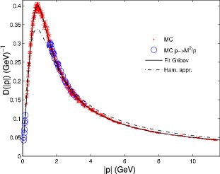
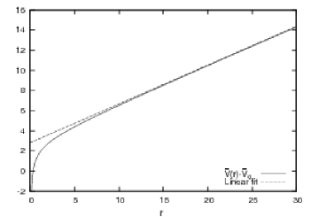
Figure 2: Static gluon propagator $1/(2\omega(k))$ compared to the lattice results (left panel) and static quark potential (right panel).

Figure 3: Running coupling constant (left panel) and dielectric function of the Yang-Mills vacuum (right panel).

In Ref. [9] it was shown that the inverse of the Coulomb gauge ghost form factor $d^{-1}(k)$ can be interpreted as the dielectric function of the Yang-Mills vacuum

$$\epsilon(k)=d^{-1}(k)\hskip 2.84544pt,$$ (14)

which is shown in fig. 3 (right). By the horizon condition (12) the dielectric constant vanishes in the infrared $\epsilon(k=0)=0$, implying that the Yang-Mills vacuum is a perfect dia-electric medium, in which by Gauss’ law $\mbox{\boldmath$\nabla$\unboldmath}(\epsilon\mbox{\boldmath$E$\unboldmath})=\rho$ free colour charges cannot exist and thus have to be confined in colourless states. This is precisely the picture underlying the $MIT$ bag model, which assumes that $\epsilon=0$ in the vacuum while $\epsilon=1$ inside the hadronic bags. The magnetic analogue of a perfect dia-electric medium is a superconductor for which the magnetic permeability $\mu$ defined by $B=\mu H$ vanishes ($B$-magnetic field, $H$-induction). In the usual notion of duality, meaning the interchange between electric and magnetic fields and charges, a medium with $\epsilon=0$ is a dual superconductor. Therefore, the Gribov-Zwanziger confinement scenario assuming $d^{-1}(k=0)=0$ implies by the identity (14) the dual Meissner effect in the infrared.

4 Functional renormalisation group flows

Our ansatz for the Yang-Mills vacuum wave functional can be tested by comparison with results from functional renormalisation group flows (FRG). The basic idea of the hamiltonian FRG is to add an infrared cut-off term quadratically in the quantum field $\phi$

$$\Delta S_{k}[\phi]=\frac{1}{2}\,\int d^{3}p\,\phi(p)R_{k}(p)\phi(-p)$$ (15)

to the Euclidean action, which cuts off momentum modes of the field $\phi$ with momenta $p<k$, but leaves the theory unchanged for momenta $p>k$. At large cut-off scales $k\to\Lambda_{UV}$ the theory is well under control due to asymptotic freedom and perturbation theory can be applied. In turn, for $k\to 0$ one recovers the full theory. The flow of the theory with the cut-off scale $k$ is described by the renormalisation group flow equation for the infrared regularised effective action $\Gamma_{k}[\phi]$. For cut-off terms (15) the flow equation reads

$$\partial_{t}\Gamma_{k}[\phi]=\frac{1}{2}\,\mathrm{Tr}\left[\left(\Gamma_{k}^{(2)}[\phi]+R_{k}\right)^{-1}\partial_{t}R_{k}\right],\qquad\partial_{t}\equiv k\,\frac{\partial}{\partial k}$$ (16)

where $\Gamma_{k}^{(2)}[\phi]+R_{k}$ is the inverse propagator of $\phi$ with

$$\Gamma^{(2)}_{k}[\phi]=\frac{\delta^{2}\Gamma_{k}[\phi]}{\delta\phi\delta\phi}$$ (17)

The flow equation (16) entails the evolution of the IR-regularised effective action from $k\to\infty$ where $\Gamma_{k}[\phi]$ coincides with the bare action $S[\phi]$ to $k\to 0$ where $\Gamma_{k}[\phi]$ is the full effective action.

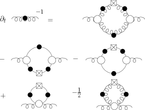
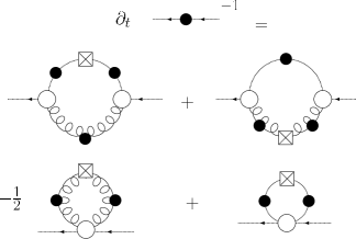
Figure 4: FRG-flows for the propagators.

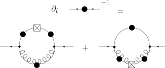
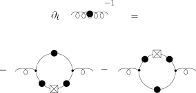
Figure 5: FRG-flows for the propagators assuming ghost dominance and dropping the tadpoles.

Here we only are interested in the flow of the propagators, which is obtained from (16) by taking the second functional derivative with respect to the fields

$$\partial_{t}\Gamma_{k}^{(2)}=\frac{\delta^{2}}{\delta\phi\,\delta\phi}\frac{1}{2}\,\mathrm{Tr}\left[\left(\Gamma_{k}^{(2)}[\phi]+R_{k}\right)^{-1}\partial_{t}R_{k}\right]\biggr{|}_{\phi=0}\>.$$ (18)

This equation is diagrammatically illustrated in fig. 4 for the propagators of Yang-Mills theory and is structurally similar to a Dyson-Schwinger equation except that the infrared regulator $\partial_{t}R_{k}$ enters the loops and all vertices and propagators are fully dressed. For the Hamiltonian flow of Yang-Mills theory in Coulomb gauge the fields involved are the transversal gauge field and the ghost field. Thus the right-hand side of the flow equation (18) receives contributions from ghost and gluon loops. We assume ghost dominance and keep only the contributions from the ghost loop to the right-hand side of the flow equation (18). The resulting flow equations for the gluon and ghost propagators are diagrammatically illustrated in fig. 5. With our choice of the vacuum wave functional the action is given by

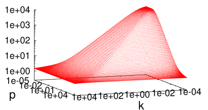
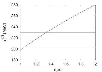
Figure 6: FRG-flow of the ghost form factor $d(p)$ (left panel). Topological susceptibility obtained in the variational approach from solution $ii)$ (11) as function of $\sigma_{c}/\sigma$ (right panel). The two horizontal lines limit the range of the lattice results.

$$S[A,c,\bar{c}]=\int A\,\omega\,A+\int\bar{c}(-\hat{D}\partial)c\hskip 2.84544pt.$$ (19)

We solve the FRG flows shown in fig. 5 for the gluon energy $\omega(p)$ and the ghost form factor $d(p)$ using the following regulators

$$\mbox{gluon:}\ R_{k}(p)\simeq p\>\exp\left(\frac{k^{2}}{p^{2}}-\frac{p^{2}}{k^{2}}\right)\;,\qquad\mbox{ghost:}\ R_{k}(p)\simeq p^{2}\>\exp\left(\frac{k^{2}}{p^{2}}-\frac{p^{2}}{k^{2}}\right)\,,\hskip 2.84544pt$$ (20)

where we have suppressed the tensor structure, and perturbative initial conditions at large cut-off scale $k=\Lambda$

$$\omega_{\Lambda}(p)=p+const\;,\qquad d_{\Lambda}(p)=const\hskip 2.84544pt$$ (21)

down to some minimal momentum cut-off scale $k_{min}$. Fig. 6 illustrates the renormalisation group flow of the ghost form factor. As the cut-off scale $k$ is reduced the ghost form factor as function of the momentum $p$ gets infrared enhanced and eventually becomes infrared divergent as the cut-off scale $k$ becomes very small, i.e. the horizon condition emerges when the infrared cut-off is removed. This is nicely seen in fig. 7 where the ghost form factor is shown at the minimum cut-off $k_{min}$ as a function of the momentum $p$. It is also seen that the infrared exponent, i.e. the slope of the curve $d_{k_{min}}(p)$, does not change as the minimal cut-off scale is lowered. Fig. 8 shows the corresponding result of the integration of the flow equation for the gluon energy $\omega_{k_{min}}(p)$. The infrared exponents of the gluon energy and the ghost form factor satisfy the sum rule (10) found from the Dyson-Schwinger equation of the variational approach. It can be shown that the FRG results coincide analytically with those of the variational approach either for optimised regulators [10], or if the ghost tadpoles are included. From analogous studies in the Landau gauge [11] we expect that for general regulators the infrared exponents are smaller. Indeed this is the case for the approximation illustrated in fig. 5 and with the regulators (20). This can be seen from figs. 7 and 8. The gaps between the solutions in figs. 7 and 8 and the difference in the exponents gives an estimate for the systematic error of the present approximation. A detailed analysis will be provided elsewhere.

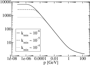
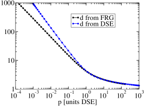
Figure 7: Ghost form factor $d_{k}(p)$ (left panel). For sake of comparison the result of the variational approach is also shown (right panel).

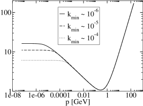
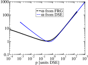
Figure 8: Gluon energy $\omega_{k}(p)$ obtained from the solution of the RG-flow equation (left panel). For sake of comparison the result of the variational approach is also shown (right panel).

5 Physical applications

An important quantity for hadron physics is the topological susceptibility $\chi$ defined by

$$\chi=\int d^{4}x\>\langle 0|q(x)\,q(0)|0\rangle\hskip 2.84544pt,\qquad q(x)=\frac{g^{2}}{8\pi^{2}}\>\mbox{\boldmath$E$\unboldmath}(x)\mbox{\boldmath$B$\unboldmath}(x)\hskip 2.84544pt,$$ (22)

where $q(x)$ is the topological charge density. It reflects the anomalous $U(1)$ symmetry breaking in QCD and can be extracted from the $\eta^{\prime}$ mass through the Witten-Veneziano formula

$$m^{2}_{\eta^{\prime}}+m^{2}_{\eta}-2m^{2}_{K}=\frac{6}{F_{\pi}^{2}}\>\chi\hskip 2.84544pt,\qquad F_{\pi}=93\mbox{ MeV}.$$ (23)

This quantity vanishes to all orders in perturbation theory and is therefore perfectly suited to test non-perturbative methods. $\chi$ is a manifestation of the $\theta-$vacuum and can be easily evaluated in the Hamiltonian approach. Adding the topological term ${\cal L}_{top}=\theta\int d^{4}x\;q(x)$ to the Yang-Mills Lagrangian shifts the momentum by $\mbox{\boldmath$\Pi$\unboldmath}\to\mbox{\boldmath$\Pi$\unboldmath}-\theta\,\frac{g^{2}}{8\pi^{2}}\,\mbox{\boldmath$B$\unboldmath}$ and the Hamiltonian of the $\theta-$vacuum reads

$$H_{\theta}=\frac{1}{2}\int\left[\left(\Pi-\theta\,\frac{g^{2}}{8\pi^{2}}\,B\right)^{2}+B^{2}\right],$$ (24)

from which one derives the following expression for the topological susceptibility ($V$ is the spatial volume)

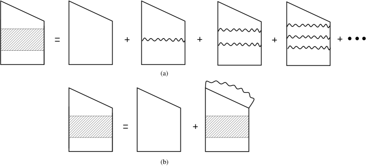
Figure 9: Graphical illustration to (a) the Dyson series for the Wilson loop and (b) the Dyson equation (26).

$$V\chi=\left.\frac{d^{2}\langle H_{\theta}\rangle}{d\theta^{2}}\right|_{\theta=0}\hskip 2.84544pt.$$ (25)

Using the Yang-Mills wave functional obtained from the variational principle for the solution $ii)$ (11) and restricting the intermediate states in eq. (25) to 3-gluon states (on top of the vacuum) one finds [12] the results shown in fig. 6 (right panel), where $\chi$ is plotted as function of the ratio $\sigma_{c}/\sigma$. $\sigma_{c}$ is the Coulomb string tension, which is extracted from the static colour potential and used to fix the scale in the variational calculations while $\sigma$ is the Wilsonian string tension extracted from the Wilson loop. Lattice calculations indicate that this ratio is in the range of $\sigma_{c}/\sigma=1.5.$ For such ratios the value obtained for $\chi$ is somewhat larger than the quenched lattice results.
A crucial test for a wave functional would be the calculation of the Wilson loop, the order parameter of the Yang-Mills theory. The spatial Wilson loop can in principle be directly calculated in the Hamiltonian approach, once the vacuum wave functional is known. However, the practical calculation is rendered difficult by the path ordering. A quantity more easily accessible is the ’t Hooft loop, the disorder parameter of Yang-Mills theory. In Ref. [13] the ’t Hooft loop was calculated using the wave functional corresponding to the solution $ii)$ (11) and a perimeter law was found, which is characteristic of the confinement phase. For further details we refer the reader to Ref. [13].

6 Wilson loop from a Dyson equation

Although the temporal Wilson loop is dual to the spatial t’Hooft loop and a perimeter law in the latter implies an area law in the former, one would appreciate an explicit calculation of the Wilson loop and observe the emergence of the area law. Recently, a Dyson equation has been proposed in the context of supersymmetric Yang-Mills theory, which, at least in an approximate fashion, takes care of the path ordering [14]. It has been applied to the temporal Wilson loop in non-supersymmetric Yang-Mills theory [15].
This Dyson equation applies to trapezoidal loops $W\left(S,T;L\right)$ and basically sums up the ladder diagrams shown in fig. 9(a), i.e. the gluon exchange between one pair of opposite paths. This Dyson equation is diagrammatically shown in fig. 9(b) and is analytically given by

$$W(S,T;L)=1+g^{2}C_{2}\int\limits^{S}_{0}ds\int\limits^{T}_{0}dtD\left(\left(x(s)-s(t)\right)^{2}\right)W(s,t;L)\hskip 2.84544pt.$$ (26)

Figure 10: (a) Processes involved and (b) processes ignored in the Dyson equation (26).

This equation suffers from the following limitations [16]:

1. Since we include only one pair of paths (see fig. 10(a)) the Dyson equation (26) is restricted to strongly asymmetric loops. However, it is irrelevant whether the loop is a temporal or spatial one.

2. When one of the two parallel temporal lines is set to zero, the trapezoidal loop degenerates to a triangle-shaped loop. In this case the Dyson equation (26) yields for the Wilson loop

   $$W\left(S,T=0;L\right)=1$$ (27)

   which, in general, is certainly incorrect. This wrong boundary condition is not surprising, since setting $T=0$ or $S=0$ contradicts the assumption $S,T\gg L$ in the Dyson equation (26).

3. The equation is bounded to produce strict Casimir scaling, which is known to occur only in the intermediate distance regime.

4. The Wilson loop is a gauge-invariant object. However, the right-hand side of the Dyson equation (26) depends via the gluon propagator on the gauge. In fact, the gluon propagator can be defined only in a gauge-fixed theory and vanishes if the gauge is unfixed.

5. Finally, the Wilson loop is renormalisation group invariant, while the right-hand side of the Dyson equation (26) is not, except for the temporal Wilson loops in Coulomb gauge (which we will consider at first).

In Coulomb gauge the temporal gluon propagator has the form

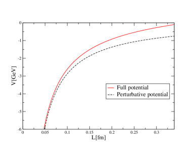
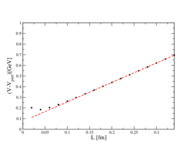
Figure 11: Left panel: The Wilsonian potential $V(L)$ obtained from the static gluon propagator (13) and the perturbative potential $V_{\text{pert}}(L)$. Right panel: The full potential minus its perturbative part.

$$g^{2}D^{ab}_{00}(x,y)=-\delta^{ab}V_{C}(|\mbox{\boldmath$x$\unboldmath}-\mbox{\boldmath$y$\unboldmath}|)\delta(x^{0}-y^{0})+P^{ab}(x,y)\hskip 2.84544pt$$ (28)

where $V_{C}(|\mbox{\boldmath$x$\unboldmath}-\mbox{\boldmath$y$\unboldmath}|)$ is the so-called non-Abelian Coulomb potential. At small distances it has the ordinary Coulombic $\sim 1/r$ behaviour, while it rises linearly at large distances $\sim\sigma_{c}r$, with $\sigma_{c}$ being the Coulomb string tension, which is larger than the Wilsonian string tension $\sigma$. The non-instantaneous part $P(x,y)$ is assumed to lower $\sigma_{c}$ towards $\sigma$. If we ignore the screening part $P(x,y)$, the gluon propagator is instantaneous and the Dyson equation (26) applies only to rectangular loops $\overline{W}\left(T;L\right)\equiv W\left(S=T,T;L\right)$

$$\overline{W}(T;L)=1-C_{2}V_{C}(L)\int\limits^{T}_{0}dt\overline{W}(t;L)\hskip 2.84544pt.$$ (29)

This equation contains the correct boundary condition $\overline{W}\left(T=0;L\right)=1$ and can be solved analytically, yielding

$$\overline{W}(T;L)=\exp\left(-C_{2}V_{C}(L)T\right)\hskip 2.84544pt.$$ (30)

Within the approximation used for the gluon propagator, we have correctly obtained an area law. It is clear why in this case the equation produces the correct result: The processes neglected in the Dyson equation (26) (see fig. (10(b)) do not exist for an instantaneous gluon propagator.
For arbitrary (non-instantaneous) gluon propagators, the Dyson equation (26) can be converted into a one-dimensional Schrödinger equation

$$\left[-\frac{d^{2}}{dr^{2}}+U(r)\right]\varphi_{n}(r)=-\frac{\Omega^{2}_{n}}{4}\varphi_{n}(r)\hskip 2.84544pt$$ (31)

with the variable $r=\frac{S-T}{L}$ and the Schrödinger potential given by

$$U(r)=-g^{2}C_{2}\,L^{2}\,D\left(L^{2}(1+r^{2})\right)\hskip 2.84544pt.$$ (32)

The Wilsonian potential can be obtained from the ”ground state energy”

$$V\left(L\right)=-\lim_{T\to\infty}\,\frac{1}{T}\ln W\left(T,T;L\right)=-\frac{\Omega_{0}\left(L\right)}{L}+const\;.$$ (33)

Applying the Dyson equation to the spatial Wilson loop in Coulomb gauge and using the static transversal gluon propagator (13) augmented by its anomalous dimension (derived in Ref. [17]) to make the gluon propagator well-defined in coordinate space, one finds the Wilsonian potential shown in fig. 11(a). When one subtracts from this potential the perturbative one, a linearly rising potential is left, implying an area law for the spatial Wilson loop, see fig. 11(b).

References

-
[1]
C. Feuchter and H. Reinhardt,
Phys. Rev. D70, 105021 (2004); [hep-th/0408236].
C. Feuchter and H. Reinhardt, [hep-th/0402106]. - [2] A. P. Szczepaniak and E. S. Swanson, Phys. Rev. D65, 025012 (2001); [hep-ph/0107078].
- [3] A. P. Szczepaniak, Phys. Rev. D69, 074031 (2004); [hep-ph/0306030].
- [4] H. Reinhardt and C. Feuchter, Phys. Rev. D 71, 105002 (2005); [hep-th/0408237].
- [5] W. Schleifenbaum, M. Leder, and H. Reinhardt, Phys. Rev. D73, 125019 (2006); [hep-th/0605115].
- [6] D. Epple, H. Reinhardt, and W. Schleifenbaum, Phys. Rev. D75, 045011 (2007); [hep-th/0612241].
- [7] D. Epple, H. Reinhardt, W. Schleifenbaum, and A. P. Szczepaniak, Phys. Rev. D77, 085007 (2008); [hep-th/0712.3694].
- [8] G. Burgio, M. Quandt and H. Reinhardt, Phys. Rev. Lett. 102 (2009) 032002; [hep-lat/0807.3291].
- [9] H. Reinhardt, Phys. Rev. Lett. 101 (2008) 061602; [hep-th/0803.0504].
-
[10]
J. M. Pawlowski,
Annals Phys. 322 (2007) 2831
[hep-th/0512261];
D. F. Litim, Phys. Lett. B 486 (2000) 92 [hep-th/0005245]. - [11] J. M. Pawlowski, D. F. Litim, S. Nedelko and L. von Smekal, Phys. Rev. Lett. 93 (2004) 152002; [hep-th/0312324].
- [12] D. R. Campagnari and H. Reinhardt, Phys. Rev. D78 (2008) 085001; [hep-th/0807.1195].
- [13] H. Reinhardt and D. Epple, Phys. Rev. D76, 065015 (2007); [hep-th/0706.0175].
-
[14]
J. K. Erickson, G. W. Semenoff, R. J. Szabo and K. Zarembo,
Phys. Rev. D61, 105006 (2000);
[hep-th/9911088].
J. K. Erickson, G. W. Semenoff and K. Zarembo, Nucl. Phys. B582, 155 (2000); [hep-th/0003055]. - [15] A. V. Zayakin and J. Rafelski, Phys. Rev. D80, 034024 (2009); [hep-ph/0905.2317].
- [16] M. Pak and H. Reinhardt, [hep-th/0910.2916].
- [17] D. Campagnari, A. Weber, H. Reinhardt, F. Astorga and W. Schleifenbaum, [hep-th/0910.4548].