Nonlinear dynamics of phase separation in thin films

Abstract

We present a long-wavelength approximation to the Navier–Stokes Cahn–Hilliard equations to describe phase separation in thin films. The equations we derive underscore the coupled behaviour of free-surface variations and phase separation. We introduce a repulsive substrate-film interaction potential and analyse the resulting fourth-order equations by constructing a Lyapunov functional, which, combined with the regularizing repulsive potential, gives rise to a positive lower bound for the free-surface height. The value of this lower bound depends on the parameters of the problem, a result which we compare with numerical simulations. While the theoretical lower bound is an obstacle to the rupture of a film that initially is everywhere of finite height, it is not sufficiently sharp to represent accurately the parametric dependence of the observed dips or ‘valleys’ in free-surface height. We observe these valleys across zones where the concentration of the binary mixture changes sharply, indicating the formation of bubbles. Finally, we carry out numerical simulations without the repulsive interaction, and find that the film ruptures in finite time, while the gradient of the Cahn–Hilliard concentration develops a singularity.

I Introduction

Below a certain critical temperature, a well-mixed binary fluid spontaneously separates into its component parts, forming domains of pure liquid. This process can be characterised by the Cahn–Hilliard equation, and numerous studies describe the physics and mathematics of phase separation CH_orig ; Bray_advphys ; Elder1988 ; Zhu_numerics ; ONaraigh2006 . In this paper we study phase separation in a thin layer, in which the varying free-surface and concentration fields are coupled through a pair of nonlinear evolution equations.

Cahn and Hilliard introduced their eponymous equation in CH_orig to model phase separation in a binary alloy. Since then, the model has been used in diverse applications: to describe polymeric fluids Aarts2005 , fluids with interfacial tension Spelt2007 ; LowenTrus , and self-segregating populations in biology Murray1981 . An analysis of the Cahn–Hilliard (CH) equation was given by Elliott and Zheng Elliott_Zheng , where they obtain existence, uniqueness, and regularity results. Several authors have developed generalisations of the CH equation: a variable-mobility model was introduced by Elliott and Garcke Elliott_varmob , while nonlocal effects were considered by Gajweski and Zacharias Gajewski_nonlocal . These additional features do not qualitatively change the phase separation, and we therefore turn to one mechanism that does: the coupling of a flow field to the Cahn–Hilliard equation Bray_advphys . In this case, the Cahn–Hilliard concentration equation is modified by an advection term, and the flow field is either prescribed or evolves according to some fluid equation. Ding and co-workers Spelt2007 provide a derivation of coupled Navier–Stokes Cahn–Hilliard (NSCH) equations in which the velocity advects the phase-separating concentration field, while concentration gradients modify the velocity through an additional stress term in the momentum equation. A similar model has been produced by Lowengrub and Truskinowsky LowenTrus . Such models have formed the basis of numerical studies of binary fluids Berti2005 , while other studies without this feedback term highlight different regimes of phase separation under flow chaos_Berthier ; ONaraigh2006 ; Lacasta1995 . Here, the NSCH equations form the starting point for our asymptotic analysis.

As in other applications involving the Navier–Stokes equations, the complexity of the problem is reduced when the fluid is spread thinly on a substrate, and the upper vertical boundary forms a free surface Oron1997 ; Matar2009 . Then, provided lateral gradients are small compared to vertical gradients, a long-wavelength approximation is possible, in which the full equations with a moving boundary at the free surface are reduced to a single equation for the free-surface height. In the present case, the reduction yields two equations: one for the free surface, and one for the Cahn–Hilliard concentration. The resulting thin-film Stokes Cahn–Hilliard equations have already been introduced by the authors in ONaraigh2007 , although the focus there was on control of phase separation and numerical simulations in three dimensions. Here we confine ourselves to the two-dimensional case: we derive the thin-film equations from first principles, present analysis of the resulting equations, and highlight the impossibility of film rupture, once a regularizing potential is prescribed. We use numerical simulations to show that in the absence of this regularizing potential, the film does indeed rupture, an event that coincides with the development of a singularity in the concentration gradient.

Along with the simplification of the problem that thin-film theory provides, there are many practical reasons for studying phase separation in thin layers. Thin polymer films are used in the fabrication of semiconductor devices, for which detailed knowledge of film morphology is required Karim2002 . Other industrial applications of polymer films include paints and coatings, which are typically mixtures of polymers. One potential application of the thin-film Cahn–Hilliard theory is in self-assembly Krausch1994 ; Xia2004 ; Lu2005 ; Putkaradze2005 ; Kim2006 . Here molecules (usually residing in a thin layer) respond to an energy-minimisation requirement by spontaneously forming large-scale structures. Equations of Cahn–Hilliard type have been proposed to explain the qualitative features of self-assembly Putkaradze2005 ; Holm2005 , and knowledge of variations in the film height could enhance these models. Indeed in ONaraigh2007 the authors use the present thin-film Cahn–Hilliard model in three dimensions to control phase separation, a useful tool in applications where it is necessary for the molecules in the film to form a given structure.

The mathematical analysis of thin-film equations was given great impetus by Bernis and Friedman in Friedman1990 . They focus on the basic thin-film equation,

$$\frac{\partial h}{\partial t}=-\frac{\partial}{\partial x}\left(h^{n}\frac{\partial^{3}{h}}{\partial{x^{3}}}\right),$$ (1)

with no-flux boundary conditions on a line segment, and smooth nonnegative initial conditions. For $n=1$ this equation describes a thin bridge between two masses of fluid in a Hele–Shaw cell, for $n<3$ it is used in slip models as $h\rightarrow 0$ Myers1998 , while for $n=3$ it gives the evolution of the free surface of a thin film experiencing capillary forces Oron1997 . Using a decaying free-energy functional, they analyzed Eq. (1) and obtained results concerning the existence, uniqueness, and regularity of solutions, as a function of the exponent $n$. Only for $n\geq 4$ does a classical, smooth solution exist; this fact is established by construction of an entropy functional. This paper Friedman1990 has inspired other work on the subject Bertozzi1996 ; Bertozzi1998 ; Laugesen2002 , in which the effect of a Van der Waals term on Eq. (1) is investigated. These works provide results concerning regularity, long-time behaviour, and film rupture in the presence of an attractive Van der Waals force. More relevant to the present work is the paper by Wieland and Garcke Wieland2006 , in which a pair of partial differential equations describes the coupled evolution of free-surface variations and surfactant concentration. The authors derive the relevant equations using the long-wavelength theory, obtain a decaying energy functional, and prove results concerning the existence and non-negativity of solutions.

When the binary fluid forms a thin film on a substrate, we shall show in Sec. II that a long-wave approximation simplifies the density- and viscosity-matched Navier–Stokes Cahn–Hilliard equations, which reduce to a pair of coupled evolution equations for the free surface and concentration. If $h(x,t)$ is the scaled free-surface height, and $c(x,t)$ is the binary fluid concentration, then the dimensionless equations take the form

$$\frac{\partial h}{\partial t}+\frac{\partial J}{\partial x}=0,\qquad\frac{\partial}{\partial t}\left(hc\right)+\frac{\partial}{\partial x}\left(Jc\right)=\frac{\partial}{\partial{x}}\left(h\frac{\partial\mu}{\partial{x}}\right),$$ (2a)

where

$$J=\tfrac{1}{2}h^{2}\frac{\partial\sigma}{\partial{x}}-\tfrac{1}{3}h^{3}\bigg{\{}\frac{\partial}{\partial{x}}\left(-\frac{1}{C}\frac{\partial^{2}{h}}{\partial{x}^{2}}+\phi\right)+\frac{r}{h}\frac{\partial}{\partial{x}}\left[h{\left(\frac{\partial{c}}{\partial{x}}\right)}^{2}\right]\bigg{\}},$$ (2b)

$$\mu=c^{3}-c-\frac{C_{\mathrm{n}}^{2}}{h}\frac{\partial}{\partial{x}}\left(h\frac{\partial{c}}{\partial{x}}\right).$$ (2c)

Here $C$ is the capillary number, $r$ measures the strength of coupling between the concentration and free-surface variations (backreaction), and $C_{\mathrm{n}}$ is the scaled interfacial thickness — sometimes called the Cahn number. Additionally, $\sigma$ is the dimensionless, spatially-varying surface tension, and $\phi$ is the body-force potential acting on the film. In this paper we focus on a class of potentials that models a repulsive interaction between the film and the substrate, thus preventing rupture. This enables us to focus on late-time phase separation, which is synonymous with a tendency to equilibrium. However, rupture is in itself an important feature in thin-film equations Oron1997 ; Bertozzi1996 ; Bertozzi1998 : we therefore use numerical methods to highlight the possibility of rupture in the absence of a repulsive film-substrate interaction.

The paper is organised as follows. In Sec. II we discuss the Navier–Stokes Cahn–Hilliard equation and the scaling laws that facilitate the passage to the long-wavelength equations, and we derive Eq. (2c). In Sec. III we perform linear and non-linear analyses of the long-wavelength equations. Our non-linear analysis centres on finding a Lyapunov functional for a given class of potentials. We derive a priori bounds for a given positive ($h>0$) solution, and estimate the minimum value of the free-surface height. In Sec. IV we outline a series of numerical studies, with and without a regularizing potential, and we discuss the dependence of the minimum free-surface height on the problem parameters. Finally, in Sec. V we present our conclusions.

II The model equations: derivation

In this section we introduce the two-dimensional Navier–Stokes Cahn–Hilliard (NSCH) equation set. We focus on the so-called matched case, wherein both components of the binary mixture have the same density and viscosity. We discuss the assumptions underlying the long-wavelength approximation. We enumerate the scaling rules necessary to obtain the simplified equations. Finally, we arrive at a set of equations that describe phase separation in a thin film subject to arbitrary body forces.

The full NSCH equations describe the coupled effects of phase separation and flow in a binary fluid. If the fluids are density- and viscosity matched, then the models described in the references Spelt2007 ; LowenTrus agree; this is the case we study. If $\bm{v}$ is the fluid velocity and $c$ is the concentration of the mixture, where $c=\pm 1$ indicates total segregation, then these fields evolve as

$$\frac{\partial\bm{v}}{\partial t}+\bm{v}\cdot\nabla\bm{v}=\nabla\cdot T-\frac{1}{\rho}\nabla\phi,$$ (3a)

$$\frac{\partial c}{\partial t}+\bm{v}\cdot\nabla c=D\nabla^{2}\left(c^{3}-c-\gamma\nabla^{2}c\right),$$ (3b)

$$\nabla\cdot\bm{v}=0,$$ (3c)

where

$$T_{ij}=-\frac{p}{\rho}\delta_{ij}+\nu\left(\frac{\partial v_{i}}{\partial x_{j}}+\frac{\partial v_{j}}{\partial x_{i}}\right)-\beta\gamma\frac{\partial c}{\partial x_{i}}\frac{\partial c}{\partial x_{j}}$$ (4)

is the stress tensor, $p$ is the fluid pressure, $\phi$ is the body potential and $\rho$ is the constant density. The constant $\nu$ is the kinematic viscosity, $\nu=\eta/\rho$, where $\eta$ is the dynamic viscosity. Additionally, $\beta$ is a constant with units of $[\mathrm{Energy}][\mathrm{Mass}]^{-1}$, $\sqrt{\gamma}$ is a constant that gives the typical width of interdomain transitions, and $D$ a diffusion coefficient with dimensions $[\mathrm{Length}]^{2}[\mathrm{Time}]^{-1}$.

We impose the following boundary conditions (BCs). On the lateral boundaries ($x$-direction), the velocity must satisfy the no-slip condition, while $c_{x}$ and $c_{xxx}$ must vanish too. Alternatively, we may enforce periodicity, and demand that the velocity, $c$, $c_{x}$, and $c_{xx}$ be periodic functions of the lateral coordinate. Finally, if the system has a free surface in the vertical or $z$-direction, then the vertical BCs are the following:

$$u=w=c_{z}=c_{zzz}\text{ on }z=0,$$ (5a)

while on the free surface $$z=h(x,t)$$ they are

$$\hat{n}_{i}\hat{n}_{j}T_{ij}=-\sigma\kappa,\qquad\hat{n}_{i}\hat{t}_{j}T_{ij}=-\frac{\partial\sigma}{\partial s},$$ (5b)

$$w=\frac{\partial h}{\partial t}+u\frac{\partial h}{\partial x},$$ (5c)

$$\hat{n}_{i}\partial_{i}c=0,\qquad\hat{n}_{i}\partial_{i}\nabla^{2}c=0,$$ (5d)

where $\hat{\bm{n}}=(-\partial_{x}{h}\,,\,1)/{[{1+(\partial_{x}{h})^{2}}]^{1/2}}$ is the unit normal to the surface, $\hat{\bm{t}}$ is the unit vector tangent to the surface, $s$ is the surface coordinate, $\sigma$ is the surface tension, and $\kappa$ is the mean curvature,

$$\kappa=\nabla\cdot\hat{\bm{n}}=\frac{\partial_{xx}h}{\left[1+\left(\partial_{x}{h}\right)^{2}\right]^{\frac{3}{2}}};$$

these free-surface conditions are standard and are discussed in the review papers Oron1997 ; Matar2009 . This choice of BCs guarantees the conservation of the total mass and volume,

$$\text{Mass}=\int_{\text{Dom}(t)}dxdz\,c(x,z,t),\qquad\text{Volume}=\int_{\text{Dom}(t)}dxdz.$$ (6)

Here $\text{Dom}(t)$ represents the time-dependent domain of integration, owing to the variability of the free-surface height. Note that in view of the concentration BC (5d), the stress BC (5b) and does not contain $c(\bm{x},t)$ or its derivatives.

These equations simplify considerably if the fluid forms a thin layer of mean thickness $h_{0}$, for then the scale of lateral variations $\ell$ is large compared with the scale of vertical variations $h_{0}$. Specifically, the parameter $\delta=h_{0}/\ell$ is small, and after nondimensionalisation of Eq. (3) we expand its solution in terms of this parameter, keeping only the lowest-order terms. For a review of this method and its applications, see Oron1997 ; Matar2009 . For simplicity, we shall work in two dimensions, but the generalisation to three dimensions is easily effected ONaraigh2007 .

In terms of the small parameter $\delta$, the equations nondimensionalise as follows. The diffusion time scale is $t_{0}=\ell^{2}/D=h_{0}^{2}/\left(\delta^{2}D\right)$ and we choose this to be the unit of time. Then the unit of horizontal velocity is $u_{0}=\ell/t_{0}=\delta D/h_{0}$ so that $u=\left(\delta D/h_{0}\right)U$, where variables in upper case denote dimensionless quantities. Similarly, the vertical velocity is $w=\left(\delta^{2}D/h_{0}\right)W$, and the free-surface height is $h=h_{0}H$. The dimensionless coordinates are introduced through the equations $x=\ell X$, $z=h_{0}Z$. Finally, for the equations of motion to be half-Poiseuille at $O\left(1\right)$ (in the absence of the backreaction) we choose $p=\left(\eta D/h_{0}^{2}\right)P$ and $\phi=\left(\eta D/h_{0}^{2}\right)\Phi$. We also stipulate the following form for the surface tension:

$$\sigma=\sigma_{0}\left[1+\delta^{q}f\left(X\right)\right],$$

where the exponent $q$ is yet to be determined. Using these scaling rules, the dimensionless momentum equations are

$$\delta Re\left(\frac{\partial U}{\partial T}+U\frac{\partial U}{\partial X}+W\frac{\partial U}{\partial Z}\right)=-\frac{\partial}{\partial X}\left(P+\Phi\right)+\delta^{2}\frac{\partial^{2}U}{\partial X^{2}}+\frac{\partial^{2}U}{\partial Z^{2}}\\ -\tfrac{1}{2}\frac{\beta\gamma}{\nu D}\frac{\partial}{\partial X}\bigg{[}\delta^{2}\left(\frac{\partial c}{\partial X}\right)^{2}+\left(\frac{\partial c}{\partial Z}\right)^{2}\bigg{]}-\frac{\beta\gamma}{\nu D}\frac{\partial c}{\partial X}\bigg{[}\delta^{2}\frac{\partial^{2}c}{\partial X^{2}}+\frac{\partial^{2}c}{\partial Z^{2}}\bigg{]},$$ (7)

$$\delta^{3}Re\left(\frac{\partial W}{\partial T}+U\frac{\partial W}{\partial X}+W\frac{\partial W}{\partial Z}\right)=-\frac{\partial}{\partial Z}\left(P+\Phi\right)+\delta^{4}\frac{\partial^{2}W}{\partial X^{2}}+\delta^{2}\frac{\partial^{2}W}{\partial Z^{2}}\\ -\tfrac{1}{2}\frac{\beta\gamma}{\nu D}\frac{\partial}{\partial Z}\bigg{[}\delta^{2}\left(\frac{\partial c}{\partial X}\right)^{2}+\left(\frac{\partial c}{\partial Z}\right)^{2}\bigg{]}-\frac{\beta\gamma}{\nu D}\frac{\partial c}{\partial Z}\bigg{[}\delta^{2}\frac{\partial^{2}c}{\partial X^{2}}+\frac{\partial^{2}c}{\partial Z^{2}}\bigg{]},$$ (8)

$$\frac{\partial U}{\partial X}+\frac{\partial W}{\partial Z}=0,$$ (9)

where

$$Re=\frac{u_{0}h_{0}}{\nu}=\frac{\delta D}{\nu}=O\left(1\right).$$ (10)

The choice of ordering for the Reynolds number $Re$ allows us to recover half-Poiseuille flow at $O\left(1\right)$. We delay choosing the ordering of the dimensionless group $\beta\gamma/D\nu$ until we have examined the concentration equation, which in nondimensional form is

$$\delta^{2}\left(\frac{\partial c}{\partial T}+U\frac{\partial c}{\partial X}+W\frac{\partial c}{\partial Z}\right)\\ =\delta^{2}\frac{\partial^{2}}{\partial X^{2}}\left(c^{3}-c\right)+\frac{\partial^{2}}{\partial Z^{2}}\left(c^{3}-c\right)-\delta^{4}C_{\mathrm{n}}^{2}\frac{\partial^{4}c}{\partial X^{4}}-C_{\mathrm{n}}^{2}\frac{\partial^{4}c}{\partial Z^{4}}-2\delta^{2}C_{\mathrm{n}}^{2}\frac{\partial^{2}}{\partial X^{2}}\frac{\partial c}{\partial Z^{2}},$$ (11)

where $C_{\mathrm{n}}^{2}=\gamma/h_{0}^{2}$. By switching off the backreaction in the momentum equations (corresponding to $\beta\gamma/D\nu\rightarrow 0$), we find the trivial solution to the momentum equations, $U=W=\partial_{X}\left(P+\Phi\right)=\partial_{Z}\left(P+\Phi\right)=0$, $H=1$. The concentration boundary conditions are then $c_{Z}=c_{ZZZ}=0$ on $Z=0,1$, which forces $c_{Z}\equiv 0$ so that the Cahn–Hilliard equation is simply

$$\frac{\partial c}{\partial T}=\frac{\partial^{2}}{\partial X^{2}}\left(c^{3}-c\right)-\delta^{2}C_{\mathrm{n}}^{2}\frac{\partial^{4}c}{\partial X^{4}}.$$

To make the lubrication approximation consistent, we take

$$\delta C_{\mathrm{n}}=\widetilde{C_{\mathrm{n}}}=\delta\sqrt{\gamma}/h_{0}=O\left(1\right).$$ (12)

We now carry out a long-wavelength approximation to Eq. (11), writing $U=U_{0}+O\left(\delta\right)$, $W=W_{0}+O\left(\delta\right)$, $c=c_{0}+\delta c_{1}+\delta^{2}c_{2}+\cdots$. We examine the boundary conditions on $c(\bm{x},t)$ first. They are $\hat{\bm{n}}\cdot\nabla c=\hat{\bm{n}}\cdot\nabla\nabla^{2}c=0$ on $Z=0,H$; on $Z=0$ these conditions are simply $\partial_{Z}c=\partial_{ZZZ}c=0$, while on $Z=H$ the surface derivatives are determined by the relations

$$\hat{\bm{n}}\cdot\nabla\ \propto\ -\delta^{2}H_{X}\partial_{X}+\partial_{Z},$$

$$\hat{\bm{n}}\cdot\nabla\nabla^{2}\ \propto\ -\delta^{4}H_{X}\partial_{XXX}-\delta^{2}H_{X}\partial_{X}\partial_{ZZ}+\delta^{2}\partial_{XX}\partial_{Z}+\partial_{ZZZ}.$$

Thus, the BCs on $c_{0}$ are simply $\partial_{Z}c_{0}=\partial_{ZZZ}c_{0}=0$ on $Z=0,H$, which forces $c_{0}=c_{0}\left(X,T\right)$. Similarly, we find $c_{1}=c_{1}\left(X,T\right)$, and

$$\frac{\partial c_{2}}{\partial Z}=Z\frac{H_{X}}{H}\frac{\partial c_{0}}{\partial X},\qquad\frac{\partial^{2}c_{2}}{\partial Z^{2}}=\frac{H_{X}}{H}\frac{\partial c_{0}}{\partial X},\qquad\text{for any }Z\in\left[0,H\right].$$

In the same manner, we derive the results $\partial_{ZZZZ}c_{2}=\partial_{ZZZZ}c_{3}=0$. Using these facts, Eq. (11) becomes

$$\frac{\partial c_{0}}{\partial T}+U_{0}\frac{\partial c_{0}}{\partial X}=\\ \frac{\partial^{2}}{\partial X^{2}}\left(c_{0}^{3}-c_{0}\right)-\widetilde{C_{\mathrm{n}}}^{2}\frac{\partial^{4}c}{\partial X^{4}}+\left(3c_{0}^{2}-1\right)\frac{H_{X}}{H}\frac{\partial c_{0}}{\partial X}-2\widetilde{C_{\mathrm{n}}}^{2}\frac{\partial^{2}}{\partial X^{2}}\frac{H_{X}}{H}\frac{\partial c_{0}}{\partial X}-\widetilde{C_{\mathrm{n}}}\frac{\partial^{4}c_{4}}{\partial Z^{4}}.$$

We now integrate this equation from $Z=0$ to $H$ and use the boundary conditions

$$\frac{\partial^{3}c_{4}}{\partial Z^{3}}=0\quad\text{on}\quad Z=0,$$

$$\frac{\partial^{3}c_{4}}{\partial Z^{3}}=H_{X}\frac{\partial^{3}c_{0}}{\partial X^{3}}+H_{X}\frac{\partial}{\partial X}\left(\frac{H_{X}}{H}\frac{\partial c_{0}}{\partial X}\right)-H\frac{\partial^{2}}{\partial X^{2}}\left(\frac{H_{X}}{H}\frac{\partial c_{0}}{\partial X}\right)\quad\text{on}\quad Z=H.$$

After rearrangement, the concentration equation becomes

$$H\frac{\partial c_{0}}{\partial T}+H\langle U_{0}\rangle\frac{\partial c_{0}}{\partial X}=\\ H\frac{\partial^{2}}{\partial X^{2}}\left[c_{0}^{3}-c_{0}-\widetilde{C_{\mathrm{n}}}^{2}\frac{\partial^{2}c_{0}}{\partial X^{2}}-\widetilde{C_{\mathrm{n}}}^{2}\frac{H_{X}}{H}\frac{\partial c_{0}}{\partial X}\right]+\frac{\partial H}{\partial X}\frac{\partial}{\partial X}\left[c_{0}^{3}-c_{0}-\widetilde{C_{\mathrm{n}}}^{2}\frac{\partial^{2}c_{0}}{\partial X^{2}}-\widetilde{C_{\mathrm{n}}}^{2}\frac{H_{X}}{H}\frac{\partial c_{0}}{\partial X}\right],$$

where

$$\langle U_{0}\rangle=\frac{1}{H}\int_{0}^{H}U_{0}\left(X,Z,T\right)dZ$$

is the vertically-averaged velocity. Introducing

$$\mu=c_{0}^{3}-c_{0}-\frac{\widetilde{C_{\mathrm{n}}}^{2}}{H}\frac{\partial}{\partial X}\left(H\frac{\partial c_{0}}{\partial X}\right),$$

the thin-film Cahn–Hilliard equation becomes

$$\frac{\partial c_{0}}{\partial T}+\langle U_{0}\rangle\frac{\partial c_{0}}{\partial X}=\frac{1}{H}\frac{\partial}{\partial X}\left(H\frac{\partial\mu}{\partial X}\right).$$ (13)

We are now able to perform the long-wavelength approximation to Eqs. (7) and (8). At lowest order, Eq. (8) is $\partial_{Z}\left(P+\Phi\right)=0$, since $c_{0}=c_{0}(X,T)$, and hence

$$P+\Phi=P_{\mathrm{surf}}+\Phi_{\mathrm{surf}}\equiv P\left(X,H(X,T),T\right)+\Phi\left(X,H(X,T),T\right).$$

We introduce a dimensionless group to measure the strength of the interaction between the concentration and velocity fields; we also specify its order of magnitude:

$$r=\frac{\delta^{2}\beta\gamma}{D\nu}=O\left(1\right).$$ (14)

Later on we refer to this quantity as the ‘backraction strength’, since it is a measure of the extent to which concentration gradients feed back into the flow field. Using this dimensionless group, Eq. (7) becomes

$$\frac{\partial^{2}U_{0}}{\partial Z^{2}}=\frac{\partial}{\partial X}\left(P_{\mathrm{surf}}+\Phi_{\mathrm{surf}}\right)+r\frac{\partial}{\partial X}\left(\frac{\partial c_{0}}{\partial X}\right)^{2}+r\frac{\partial c_{0}}{\partial X}\frac{\partial^{2}c_{2}}{\partial Z^{2}}.$$

Using $\partial_{ZZ}c_{2}=\left(H_{X}/H\right)\left(\partial c_{0}/\partial X\right)$ this becomes

$$\frac{\partial^{2}U_{0}}{\partial Z^{2}}=\frac{\partial}{\partial X}\left(P_{\mathrm{surf}}+\Phi_{\mathrm{surf}}\right)+\frac{r}{H}\frac{\partial}{\partial X}\left[H\left(\frac{\partial c_{0}}{\partial X}\right)^{2}\right].$$ (15)

At lowest order, the BC (5b) reduces to

$$\frac{\partial U_{0}}{\partial Z}=\frac{\partial\Sigma}{\partial{X}}\quad\text{on}\quad Z=H,$$ (16)

which combined with Eq. (15) yields the relation

$$\frac{\partial U_{0}}{\partial Z}=\frac{\partial\Sigma}{\partial X}+\left(Z-H\right)\bigg{\{}\frac{\partial}{\partial X}\left(P_{\mathrm{surf}}+\Phi_{\mathrm{surf}}\right)+\frac{r}{H}\frac{\partial}{\partial X}\left[H\left(\frac{\partial c_{0}}{\partial X}\right)^{2}\right]\bigg{\}}.$$

Here $\Sigma$ is the dimensionless, spatially-varying component of the surface tension. Making use of the BC $U_{0}=0$ on $Z=0$ and integrating again, we obtain the result

$$U_{0}\left(X,Z,T\right)=Z\frac{\partial\Sigma}{\partial X}+\left(\tfrac{1}{2}Z^{2}-HZ\right)\bigg{\{}\frac{\partial}{\partial X}\left(P_{\mathrm{surf}}+\Phi_{\mathrm{surf}}\right)+\frac{r}{H}\frac{\partial}{\partial X}\left[H\left(\frac{\partial c_{0}}{\partial X}\right)^{2}\right]\bigg{\}}.$$ (17)

The vertically-averaged velocity is therefore

$$\langle U_{0}\rangle=\tfrac{1}{2}H\frac{\partial\Sigma}{\partial X}-\tfrac{1}{3}H^{2}\bigg{\{}\frac{\partial}{\partial X}\left(-\frac{1}{C}\frac{\partial^{2}H}{\partial X^{2}}+\Phi_{\mathrm{surf}}\right)+\frac{r}{H}\frac{\partial}{\partial X}\left[H\left(\frac{\partial c_{0}}{\partial X}\right)^{2}\right]\bigg{\}},$$ (18)

where we used the standard Laplace–Young free-surface boundary condition to eliminate the pressure, and

$$C=\frac{\nu\rho D}{h_{0}\sigma_{0}\delta^{2}}=O\left(1\right).$$ (19)

Finally, by integrating the continuity equation in the $Z$-direction, we obtain, in a standard manner, an equation for free-surface variations,

$$\frac{\partial H}{\partial T}+\frac{\partial}{\partial X}\left(H\langle U_{0}\rangle\right)=0.$$ (20)

The inclusion of the surface-tension terms requires further elucidation. In the long-wave limit, the normal-stress condition reduces to $p|_{h}=-\sigma h_{xx}$, which in dimensionless form is

$$P=-\frac{\sigma_{0}\delta^{2}h_{0}}{\nu\rho D}\left[1+\delta^{q}f\left(x\right)\right]H_{XX}.$$

By promoting the constant $C={\nu\rho D}/\left(h_{0}\sigma_{0}\delta^{2}\right)$ to $O\left(1\right)$, and by taking $q>1$, this equation reduces to $P=-C^{-1}H_{xx}$, as in Eq. (18). Similarly, the normal-stress condition reduces to $\nu\rho\left(\partial u/\partial z\right)_{h}=\partial\sigma/\partial x$, which in dimensionless form reads

$$\frac{\partial U}{\partial Z}=\frac{\sigma_{0}h_{0}\delta^{q}}{\nu\rho D}\frac{\partial f}{\partial X}.$$

Taking $q=2$ gives a contribution to the shear-stress balance at lowest order, $\partial U/\partial Z=\partial\Sigma/\partial X$, $\Sigma=f\left(X\right)/C$, as in Eq. (16). Going to higher exponents $q>2$ suppresses this contribution.

Let us assemble our results, restoring the lower-case fonts and omitting ornamentation over the constants. The height equation (20) becomes

$$\frac{\partial h}{\partial t}+\frac{\partial J}{\partial x}=0,$$ (21a)

while the concentration equation (13) becomes

$$\frac{\partial}{\partial t}\left(ch\right)+\frac{\partial}{\partial x}\left(Jc\right)=\frac{\partial}{\partial{x}}\left(h\frac{\partial\mu}{\partial{x}}\right),$$ (21b)

where

$$J=\tfrac{1}{2}h^{2}\frac{\partial\sigma}{\partial{x}}-\tfrac{1}{3}h^{3}\bigg{\{}\frac{\partial}{\partial{x}}\left(-\frac{1}{C}\frac{\partial^{2}{h}}{\partial{x}^{2}}+\phi\right)+\frac{r}{h}\frac{\partial}{\partial{x}}\left[h\left(\frac{\partial{c}}{\partial{x}}\right)^{2}\right]\bigg{\}},$$ (21c)

and

$$\mu=c^{3}-c-C_{\mathrm{n}}^{2}\frac{1}{h}\frac{\partial}{\partial{x}}\left(h\frac{\partial{c}}{\partial{x}}\right),$$ (21d)

and where we have the nondimensional constants

$$r=\frac{\delta^{2}\beta\gamma}{D\nu},\qquad C_{\mathrm{n}}=\frac{\delta\sqrt{\gamma}}{h_{0}},\qquad C=\frac{\nu\rho D}{h_{0}\sigma_{0}\delta^{2}}.$$ (22)

The boundary conditions are inherited from the full Navier–Stokes Cahn–Hilliard equations: Since $J$ contains a depth-averaged velocity, we write it as $J:=hu$. Thus, the concentration $c$, the chemical potential $\mu$, and the flux $J$ are either periodic functions in the lateral direction, or satisfy the no-flux conditions $c_{x}=\mu_{x}=J=0$ on the lateral boundaries. Equations (21d), together with the boundary conditions described, are the thin-film NSCH equations. The integral quantities defined in Eq. (6) are manifestly conserved, while the free surface and concentration are coupled. The term $\left(h^{2}/2\right)\sigma_{x}$ in the flux $J$ represents a driving force, which can be externally prescribed, or a function of the concentration $c$. In either case, the inclusion of this term can have a substantial effect on the behaviour of the system. For the rest of this study, this term is set to zero; its inclusion is discussed elsewhere by the present authors ONaraigh2007 , and by others Oron2008 .

In view of the severe constraint $C_{\mathrm{n}}=\delta\sqrt{\gamma}/h_{0}=O\left(1\right)$, some discussion about the applicability of Eqs. (21d) to real systems is warranted. This constraint is the condition that the mean thickness of the film be much smaller than the transition-layer thickness. In experiments involving the smallest film thicknesses attainable ($10^{-8}$ m) Sung1996 , this condition is naturally satisfied. Furthermore, in certain situations far from this limiting case, variations in the domain structure in the vertical direction are suppressed, and a system of equations with no vertical ($z$-) dependence, such as Eqs. (21d), is appropriate. This kind of situation arises when external effects such as the air-fluid and fluid-substrate interactions do not prefer one binary fluid component or another; hence, the dimensionality of the film is reduced, and the balance laws implied by Eqs. (21d) are applicable.

III The model equations: analysis

The choice of potential $\phi_{0}$ determines the behaviour of solutions. In this section, we perform a linear-stability analysis on the model equations (21d) and identify the pattern-formation mechanism. We also develop results for the non-linear regime using the theory of a priori bounds. These are bounds on norms of the solution $\left(h,c\right)$ that are obtained without assuming any prior knowledge of the solution. Throughout this section, the driving force resulting from surface-tension gradients is set to zero.

The first step in our analytical study is to find the circumstances under which the constant state $\left(h_{0},c_{0}\right)$ is unstable to a small-amplitude, initial perturbation $\left(\delta h_{0},\delta c_{0}\right)$. This perturbation evolves in time to a state $\left(\delta h,\delta c\right)\left(x,t\right)$, which satisfies the linearized version of equations (21d). By writing down a wave ansatz $\left(\delta h,\delta c\right)\propto e^{ikx}$, we obtain an eigenvalue equation,

$$\frac{d}{dt}\left(\begin{array}[]{c}\delta h\\ \delta c\end{array}\right)=\left(\begin{array}[]{cc}\frac{h_{0}^{3}}{3}\left[-k^{4}-k^{2}\phi_{0}^{\prime}\left(h_{0}\right)\right]&0\\ 0&-k^{2}\left(3c_{0}^{2}-1\right)-C_{\mathrm{n}}^{2}k^{4}\end{array}\right)\left(\begin{array}[]{c}\delta h\\ \delta c\end{array}\right),$$

with eigenvalues

$$\begin{split}\lambda_{h}&=-\frac{h_{0}^{3}k^{2}}{3}\left[\frac{k^{2}}{C}+\phi_{0}^{\prime}\left(h_{0}\right)\right],\\ \lambda_{c}&=-\left(3c_{0}^{2}-1\right)k^{2}-C_{\mathrm{n}}^{2}k^{4}.\end{split}$$ (23)

Thus, there are two routes to instability. The system can become unstable as a result of substrate-film interactions if $\phi_{0}^{\prime}\left(h_{0}\right)<0$. Such an interaction will often lead to rupture Oron1997 . If this route is suppressed, then film rupture may be prevented, but the second route to instability is also relevant. This is accessible when $c_{0}$ is in the spinodal range $\left|c_{0}\right|<1/\sqrt{3}$. Thus, even when the first route to instability is not accessible, a critical mixed state will phase separate in a manner similar to the classical Cahn–Hilliard fluid, as described in Sec. I.

While the linear analysis is helpful to describe early-stage evolution, it sheds no light on the behaviour at later times. We therefore turn to the non-linear analysis of the problem (21d). The non-linear analysis centres on finding bounds for a given solution $\left(h,c\right)$. To do this, it is necessary to construct a Lyapunov functional, that is, a non-negative, non-increasing functional of the solution $\left(h,c\right)$. It is certainly the case that we can find a non-increasing functional based on the solution pair $\left(h,c\right)$, which is a kind of energy for the problem:

Proposition 1 (Existence of a decreasing functional)

Given a smooth solution $\left(h,c\right)$ to the equations (21d), positive in the sense that $h\left(x,t\right)>0$, and a continuous potential function $\phi_{0}$, then the functional

$$\mathcal{F}\left[h,c\right]=\int_{0}^{L}{dx}\,\left[\frac{1}{2C}\left(\frac{\partial{h}}{\partial{x}}\right)^{2}+\int^{h}\phi_{0}\left(s\right)ds\right]+\frac{r}{C_{\mathrm{n}}^{2}}\int_{0}^{L}{dx}\,h\left[\tfrac{1}{4}\left(c^{2}-1\right)^{2}+\frac{C_{\mathrm{n}}^{2}}{2}\left(\frac{\partial{c}}{\partial{x}}\right)^{2}\right]$$ (24)

is non-increasing, $\dot{\mathcal{F}}\leq 0$.

The proof of this claim is readily obtained by a straightforward time-differentiation of $\mathcal{F}\left[h,c\right]$ and application of the equations (21d), together with the no-flux or periodic boundary conditions. We find,

$$\dot{\mathcal{F}}=-\int_{0}^{L}dx\left(\frac{3J^{2}}{h^{3}}+h\mu_{x}^{2}\right)\leq 0.$$ (25)

We build on this result by focussing on the following class of potential whose anti-derivative is positive:

$$\phi_{1}\left(s\right):=-\int_{s}^{a}\phi_{0}\left(s^{\prime}\right)ds^{\prime}>0,\qquad 0<s<a,$$ (26)

where $a$ is an arbitrary reference height. Using Prop. 1 and the condition (26), we obtain a Lyapunov functional for the positive solution $\left(h,c\right)$, $h>0$:

Proposition 2 (Existence of a positive Lyapunov functional)

For a smooth solution $\left(h,c\right)$ to the equations (21d), positive in the sense that $h\left(x,t\right)>0$, and for a potential function $\phi_{0}$ with positive anti-derivative, there is an associated Lyapunov functional.

To verify this claim, it suffices to note that since $\phi_{1}>0$ for the class of potential functions under consideration, all terms in the functional $\mathcal{F}\left[h,c\right]$ (Eq. (24)) are positive, and thus $\mathcal{F}$ is a positive, non-increasing function of time, i.e. a Lyapunov functional.

The boundedness result $\mathcal{F}\left(t\right)\leq\mathcal{F}\left(0\right)$ provides a regularity condition on the height $h\left(x,t\right)$, although this is valid only in a single spatial dimension.

Proposition 3 (Hölder continuity of $h\left(x,\cdot\right)$)

If $\left(h,c\right)$ is a smooth, positive solution to the equations (21d), in the sense that $h\left(x,t\right)>0$, and if the potential function $\phi_{0}$ has a positive anti-derivative, then $h\left(x,\cdot\right)$ is Hölder continuous, with time-independent Hölder constant $k_{H}$.

Proposition 3 follows from the a priori bounds

$$\frac{1}{2C}\int_{0}^{L}dx\,h_{x}^{2}\leq\mathcal{F}\left(t\right)\leq\mathcal{F}\left(0\right),$$ (27)

and from the use of Hölder’s inequality on the following string of relations:

$$|h\left(x_{2}\right)-h\left(x_{1}\right)|=\left|\int_{x_{1}}^{x_{2}}h_{x}dx\right|\leq\int_{x_{1}}^{x_{2}}dx\,|h_{x}|\\ \leq|x_{2}-x_{1}|^{1/2}\sqrt{\int_{0}^{L}dx\,h_{x}^{2}}\leq k_{H}|x_{2}-x_{1}|^{1/2},$$

where $k_{H}=\sqrt{2C\mathcal{F}\left(0\right)}$ is the time-independent Hölder constant. As an immediate corollary of this result, we obtain an upper bound on the height field:

Proposition 4 (An upper bound on the height field)

If $\left(h,c\right)$ is a smooth, positive solution to the equations (21d), in the sense that $h\left(x,t\right)>0$, and if the potential function $\phi_{0}$ has a positive anti-derivative, then $h\left(x,\cdot\right)$ is bounded above.

Since the free energy contains a term in the $L^{2}$-norm of $h^{1/2}c_{x}$, a similar result exists for the concentration field, provided $h>0$ everywhere. Loss of control over the minimum value of $h$ therefore implies loss of control over the concentration gradient. This suggests that blowup of gradients and film rupture are related, a claim which we demonstrate numerically in Sec. IV.2. Such extreme events are avoided when a repulsive film-substrate interaction is present, in which case a positive lower bound on $h$ exists; it is to that result that we now turn.

Given the form of Eqs. (21d), regularity of a given solution $\left(h,c\right)$ is guaranteed only when a lower bound on $h$ is obtained, in addition to the upper bounds just provided. To derive such a result, we first specialize to the potential

$$\phi_{0}=-\frac{G}{2s^{3}},\qquad G>0.$$ (28)

from which a more general result will follow.

Proposition 5 (No-rupture condition for the potential in Eq. (28))

If $\left(h,c\right)$ is a smooth, positive solution to the equations (21d), in the sense that $h\left(x,t\right)>0$, and if the potential function $\phi_{0}$ has the form given by Eq. (28), then there is an a priori, time-independent lower bound on $h$.

Note first of all that the potential (28) has a positive anti-derivative, $\phi_{1}\left(s\right)=Gs^{-2}$, where the reference height $a$ in Eq. (26) is set to $a=\infty$. Thus, there is a Lyapunov functional for the solution $\left(h,c\right)$, and hence,

$$\int_{0}^{L}dx\,Gh^{-2}=\int_{0}^{L}dx\,\phi_{1}\left(h\right)\leq\mathcal{F}\left(t\right)\leq\mathcal{F}\left(0\right).$$ (29)

Using the Hölder continuity of $h$,

$$h^{2}\leq h_{\mathrm{min}}^{2}+2h_{\mathrm{min}}k_{H}L^{1/2}+k_{H}^{2}|x-x_{\mathrm{min}}|\leq h_{\mathrm{min}}^{2}+2h_{\mathrm{min}}k_{H}L^{1/2}+k_{H}^{2}x,$$ (30)

where $k_{H}=\sqrt{2C\mathcal{F}\left(0\right)}$ is the Hölder constant for $h$. Using results (29) and (30),

$$G\int_{0}^{L}\frac{dx}{h_{\mathrm{min}}^{2}+2h_{\mathrm{min}}k_{H}L^{1/2}+k_{H}^{2}x}\leq\mathcal{F}\left(0\right).$$ (31)

By integrating this equation, we arrive at the relation

$$\log\left(1+\frac{k_{H}^{2}L}{h_{\mathrm{min}}^{2}+2k_{H}L^{1/2}h_{\mathrm{min}}}\right)\leq\frac{\mathcal{F}\left(0\right)k_{H}^{2}}{G}.$$ (32)

Let us examine the properties of the function $\log\left[1+k_{H}^{2}L/\left(s^{2}+2k_{H}L^{1/2}s\right)\right]$. It tends to infinity as $s\rightarrow 0$, and tends to zero as $s\rightarrow\infty$. It is also monotone-decreasing over $s\in\left(0,\infty\right)$. Thus, the equation $\log\left[1+k_{H}^{2}L/\left(s^{2}+2k_{H}L^{1/2}s\right)\right]=\mathcal{F}\left(0\right)k_{H}^{2}/G$ has precisely one positive root for $\mathcal{F}\left(0\right)\neq 0$, which we call $s_{*}$. To satisfy the inequality (32), it must be the case that

$$h_{\mathrm{min}}\geq s_{*}>0.$$

For the potential $\phi_{0}=-\left(G/2\right)s^{-3}$ (Eq. (28)), the root $s_{*}$ can be obtained explicitly:

$$h_{\mathrm{min}}\geq s_{*}=k_{H}L^{1/2}\left[\sqrt{\frac{1}{\exp\left(\mathcal{F}\left(0\right)k_{H}^{2}/G\right)-1}}-1\right]>0.$$

This completes the proof of the no-rupture condition for the potential (28).

To arrive at a no-rupture condition for a general potential, we introduce the function

$$\phi_{2}\left(s\right):=\int_{0}^{L}dx\,\phi_{1}\left(s+k_{H}x^{1/2}\right).$$ (33)

Based on Prop. 5, we write down sufficient conditions on $\phi_{1}$ and $\phi_{2}$ for the existence of a positive lower bound on $h$:

Proposition 6 (A sufficient condition to avoid rupture)

If $\left(h,c\right)$ is a smooth, positive solution to the equations (21d), in the sense that $h\left(x,t\right)>0$, if the anti-derivative of the potential function $\phi_{0}$ is a positive, non-increasing function, and moreover, if $\phi_{2}$ satisfies the conditions

$$\lim_{s\rightarrow 0}\phi_{2}\left(s\right) = \infty,$$

$$\lim_{s\rightarrow\infty}\phi_{2}\left(s\right) \leq 0,$$ (34)

then a positive a priori lower bound on $h\left(x,t\right)$ exists, independent of time.

The proof of Prop. 6 is in the same spirit as that of Prop. 5. Given the positivity of the anti-derivative $\phi_{1}$, a Lyapunov exponent exists (Prop. 1), and thus we have the bound $\int dx\,\phi_{1}\left(h\right)\leq\mathcal{F}\left(0\right)$. Using the Hölder continuity of $h$ (Prop. 3), and the condition that the $\phi_{1}$ should be a non-increasing function,

$$h\left(x,t\right) \leq h_{\mathrm{min}}+k_{H}x^{1/2},$$

$$\phi_{1}\left(h\left(x,t\right)\right) \geq \phi_{1}\left(h_{\mathrm{min}}+k_{H}x^{1/2}\right).$$

Using the bound $\int dx\,\phi_{1}\left(h\right)\leq\mathcal{F}\left(0\right)$,

$$\phi_{2}\left(h_{\mathrm{min}}\right)=\int_{0}^{L}dx\,\phi_{1}\left({h_{\mathrm{min}}+k_{H}x^{1/2}}\right)\leq\mathcal{F}\left(0\right).$$

Given the conditions (34), there exists at least one solution to the equation $\phi_{2}\left(s\right)=\mathcal{F}\left(0\right)$, for $\mathcal{F}\left(0\right)>0$. Indeed, since $\phi_{1}$ is non-increasing, so too is $\phi_{2}$, and thus this equation has precisely one solution, which we call $s_{*}$. Then, for the condition $\phi_{2}\left(h_{\mathrm{min}}\right)\geq\mathcal{F}\left(0\right)$ to be satisfied on the interval $\left(0,\infty\right)$, we must take

$$h_{\mathrm{min}}\geq s_{*}>0.$$

Finally, using this theory, we investigate the potential

$$\phi_{0}=-\frac{G}{ns^{n+1}},$$ (35)

and calculate the $n$-values for which a no-rupture condition can be found.

Proposition 7 (Conditions on the potential (35) to avoid rupture)

If $\left(h,c\right)$ is a smooth, positive solution to the equations (21d), in the sense that $h\left(x,t\right)>0$, and if the potential function $\phi_{0}$ is given by Eq. (35), then a no-rupture condition is guaranteed to hold for $n\geq 2$.

The proof of Prop. 7 follows by a straightforward evaluation of the integral (33). The case $n=2$ is covered by Prop. 5. Thus, we focus on the case $n\neq 2$, where the integral $\phi_{2}\left(s\right)$ has the value

$$\phi_{2}\left(s\right)=\frac{2G}{\left(n-2\right)\left(n-1\right)k_{H}^{n}}\frac{1}{\alpha^{n-2}}\left[1-\left(\frac{\alpha}{\alpha+1}\right)^{n-1}\left(1+\frac{n-1}{\alpha}\right)\right],\qquad\alpha=s/k_{H},$$ (36)

and where we have set $L=1$. For $n>2$ the conditions (34) hold: $\lim_{s\rightarrow 0}\phi_{2}\left(s\right)=\infty$, $\lim_{s\rightarrow\infty}\phi_{2}\left(s\right)=0$; note also that $\phi_{2}\left(s\right)$ is non-increasing. Thus, the equation $\phi_{2}\left(s\right)=\mathcal{F}\left(0\right)$ has exactly one positive root $s_{*}$, and this serves as a lower bound on $h$, $h_{\mathrm{min}}\geq s_{*}>0$. Note

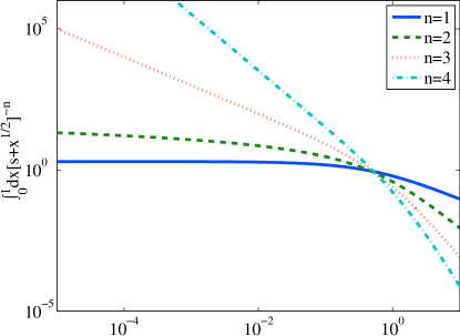
Figure 1: A plot of the integral $\int_{0}^{L}dx\left(s+x^{1/2}\right)^{-n}$ as a function of $s$. For $n\geq 2$ the integral diverges as $s\rightarrow 0$ and tends to zero as $s\rightarrow\infty$, allowing for the existence of a positive root for the equation $\int_{0}^{L}dx\left(s+x^{1/2}\right)^{-n}=\mathrm{const.}>0$.

that the relation given in Eq. (36) fails to satisfy conditions (34) when $n<2$. Thus, a sufficient condition for the solution $\left(h,c\right)$ to possess a no-rupture condition is for the potential $\phi_{0}$ to have the form given in Eq. (35), with $n\geq 2$. This analysis is also described schematically in Fig. 1, where a plot of the integral $\int_{0}^{L}dx\left(s+x^{1/2}\right)^{-n}$ is shown as a function of $s$. For $n\geq 2$ the integral diverges as $s\rightarrow 0$ and tends to zero as $s\rightarrow\infty$, which provides for the existence of a positive root for the equation $\int_{0}^{L}dx\left(s+x^{1/2}\right)^{-n}=\mathrm{const.}>0$.

Two questions arise from our results. The first involves the form of the potential used in the derivation of a no-rupture condition: can we replace the repulsive power-law form with a more general function and still obtain a no-rupture condition? The answer to this question comes readily through the observation that our construction of a positive lower bound for $h$ relies only on the surface-tension and body-force components of the free energy, namely

$$\mathcal{F}_{1}=\int_{0}^{L}dx\left[\frac{1}{2C}h_{x}^{2}+\phi_{1}\left(h\right)\right].$$

Thus, Propositions 5–7 can be viewed in the context of the PDE theory for a single variable (the free-surface height), where a no-rupture condition exists Grun2001 , both for the power-law type potential considered here and for the Lennard–Jones potential $\phi_{0}=-Gs^{-n_{1}}+Bs^{-n_{2}}$, where $G$ and $B$ are positive constants and $n_{1}>\max\left(n_{2},\min\left(1+2n_{2},3\right)\right)$ Grun2001 . Hence, our regularity results are generalizable to this wider class of potential.

Having weakened the sufficient condition for the avoidance of rupture, it is reasonable to ask, is the presence of a suitable potential even a necessary condition? This question is motivated by the single-variable theory for the free-surface height, where under certain conditions an entropy functional facilitates the construction of an a priori lower bound on the height $h\left(x,t\right)$ Friedman1990 . The entropy is obtained through the following steps, which we describe for the single-variable case $3h_{t}+\{h^{n}\left[\left(h_{xxx}/C\right)-\phi_{x}\right]\}_{x}=0$:

1. Identify the power of $h$ that is a factor in the flux $J$; this is the mobility, $m_{0}$. For the single-variable case, $m_{0}\left(h\right)=h^{n}$.

2. Obtain the function $m_{1}\left(s\right)=\int^{s}ds^{\prime}\int^{s^{\prime}}ds^{\prime\prime}\left[m\left(s^{\prime\prime}\right)\right]^{-1}$.

3. The entropy is then defined as $\mathcal{S}=\int_{0}^{L}dx\,m_{1}\left(h\right)$; for the single-variable case, this is $\mathcal{S}=\int_{0}^{L}dx\,h^{-n+2}$ (we have omitted the unimportant constant of proportionality).

For the single-variable case,

$$\mathcal{S}\left(t\right)+\frac{2}{3C}\int_{0}^{t}dt^{\prime}\int_{0}^{L}dx\,h_{xx}^{2}+\tfrac{2}{3}\int_{0}^{t}dt^{\prime}\int_{0}^{L}dx\,h_{x}^{2}\phi_{0}^{\prime}\left(h\right)=\mathcal{S}\left(0\right)>0,$$ (37)

and the entropy is a non-increasing functional of $t$, $d\mathcal{S}/dt\leq 0$. Setting $\phi_{0}=0$ in Eq. (37) gives the relation

$$\int_{0}^{L}\frac{dx}{\left[h\left(x,t\right)\right]^{n-2}}+\frac{2}{3C}\int_{0}^{t}dt^{\prime}\int_{0}^{L}dx\,h_{xx}^{2}=\mathcal{S}\left(0\right)>0.$$ (38)

For $n\geq 4$, Hölder continuity combined with the bound in Eq. (38) enables the construction of a pointwise lower bound on $h$. When $n=3$ (the case considered in this paper), no such pointwise bound exists; then, estimates for the entropy based on the Hölder continuity of $h$ are non-singular in the minimum height. However, a more definitive obstacle than this exists when we seek to construct an entropy functional for the system (21d), namely, that the entropy functional implied by Eqs. (21d) fails to be a non-increasing function of time:

Proposition 8

(The time-derivative of the entropy associated with Eqs. (21d) is not sign definite) Given a smooth, positive solution $\left(h,c\right)$ to the equations (21d), in the sense that $h\left(x,t\right)>0$, the rate of change of the functional $\int_{0}^{L}dx\,h^{\alpha}$, $\alpha<0$, is not sign-definite.

This result is established by direct computation:

$$\frac{d}{dt}\int_{0}^{L}dx\,h^{\alpha}=-\frac{\alpha\left(\alpha-1\right)}{3C}\int_{0}^{L}dx\,\left(h^{\alpha+1}h_{x}\right)_{x}{h_{xx}}\\ -\frac{\alpha\left(\alpha-1\right)}{3}\int_{0}^{L}dx\,h^{\alpha+1}h_{x}^{2}\phi_{0}^{\prime}\left(h\right)-\frac{r\alpha\left(\alpha-1\right)}{3}\int_{0}^{L}dx\,\left(h^{\alpha}h_{x}\right)_{x}hc_{x}^{2}.$$

No value of $\alpha$ can give the integral in the last term, namely

$$\int_{0}^{L}dx\,\left(h^{\alpha}h_{x}\right)_{x}hc_{x}^{2}=\int_{0}^{L}dx\left[\alpha h^{\alpha}c_{x}^{2}h_{x}^{2}+h^{\alpha+1}h_{xx}c_{x}^{2}\right]$$

a definite sign. Hence, the entropy functional fails to be non-increasing, and therefore cannot be used to construct a lower bound on $h$. The existence of a suitable potential function in the evolution equation for $h$ is thus a necessary and sufficient condition for the avoidance of rupture. Indeed, the existence of the backreaction in the equations (21d), and its consequences for the entropy functional, suggest that it promotes rupture while the regularizing potential inhibits it. To examine this effect further, we turn to numerical simulations.

IV Numerical results

In this section we obtain numerical solutions of the equations (21d), with and without the regularizing potential. Our numerical method is described and validated in Appendix A. Where present, the regularizing potential is assigned the form $\phi=-G/h^{3}$, $G>0$, which satisfies the no-rupture condition given in Sec. III. In the case where the no-rupture condition is satisfied, we study solutions that tend towards an equilibrium. We then characterize this equilibrium through the solution of a boundary-value problem. The tendency towards equilibrium is in agreement with the predictions of Sec. III, where a linearly unstable state evolves to reduce the energy functional (24), such that domains of concentration form, separated by transition zones, across which the height of the film decreases markedly, forming ‘valleys’. For the case where the no-rupture condition is not automatically satisfied ($G=0$), we perform numerical studies that suggest that rupture does indeed occur, and coincides with the development of a finite-time singularity. Throughout this section, the driving force resulting from surface-tension gradients is set to zero.

IV.1 Numerical studies with a regularizing Van der Waals potential

We perform numerical simulations of the full equations (21d), with initial data comprising a perturbation away from the unstable steady state $\left(h,c\right)=\left(1,0\right)$:

$$h\left(x,0\right)=1,\qquad c\left(x,0\right)=0.01\sin\left[5\left(2\pi/L\right)x\right].$$

We fix the parameters $G=C=1$, and $C_{\mathrm{n}}=0.1$. The $C_{\mathrm{n}}$-value is small enough such that the transition width of domains is much smaller than the size of the computational domain $L=2\pi$. We vary the parameter $r$ between $0.1$ and $1$ to examine the effects of the backreaction strength. The calculations are carried out on a periodic domain, with $N=256$ gridpoints and a timestep $\Delta t=10^{-4}$. The early-stage growth in the concentration is governed by the linear theory of Eq. (23).

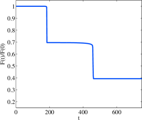
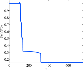
Figure 2: Numerical simulation of the decay of the free energy over time. (a) $r=0.1$; (b) $r=1$ (the other parameters are kept constant: $C=G=1$, $C_{\mathrm{n}}=0.1$). There is a very small, local increase in the free energy in case (b) due to numerical error. This is small however, and is in contrast to the otherwise decreasing trend in the free energy. The energy decreases particularly sharply when domains merge: the sharp drops correspond precisely to the domain-merging events in Fig. 3.

The free energy is a decreasing function of time (Fig. 2). The average height is conserved exactly by the numerical simulation, while the mass $\int chdx$ deviates from its initial value of zero within a range $\pm 10^{-4}$ for the $r=0.1$ case, and $\pm 10^{-2}$ for the $r=1$ case. In the course of this evolution, the amplitude of the initial sinusoidal concentration field grows transiently in time; later on the positive and negative ‘domains’ formed by each half-period of the sine function merge to form larger domains, each of larger amplitude. At the same time, the free-surface height decreases in value at the borders of these domains, forming valleys. Eventually, and as a consequence of the energy-minimization principle (25), only a single domain remains. This evolution is best described visually, as in Fig. 3, where spacetime plots of $c$ and $h$ show eventual coalescence into a pair of opposite-signed $c$-domains. The domain coalescence happens more rapidly for the $r=1$ case, compared to the $r=0.1$ case. This shows that the coupling of the free-surface height to the Cahn–Hilliard concentration far from arresting the domain coarsening, actually enhances it.

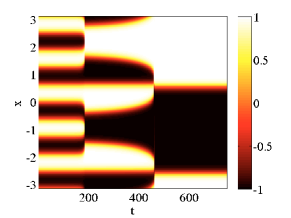
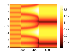
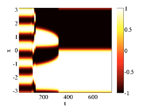
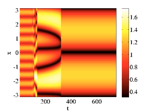
Figure 3: Temporal evolution of the free-surface and concentration fields. Across the top the backreaction strength is set to $r=0.1$. Subfigure (a) shows the concentration for this case; (b) shows the free-surface height. Across the bottom the backreaction strength has been increased to $r=1.0$. Subfigure (c) shows the corresponding concentration; (d) shows the free-surface height. The other parameters are kept constant: $C=G=1$, $C_{\mathrm{n}}=0.1$. The domains coalesce until only a pair of opposite-signed domains remain. The coalescence is more rapid for the $r=1$ case, compared to the $r=0.1$ case.

The free surface and concentration evolve to an equilibrium state where the salient feature is the formation of domains (intervals where $c\approx\pm 1$) that are separated by smooth transition zones, across which the free surface dips below its average value. We therefore shift focus to this state, obtained by setting $\mu=\mathrm{constant}$, $u=0$ in Eq. (21d):

$$\frac{1}{C}\frac{\partial^{2}h}{\partial x^{2}}=C_{\mathrm{n}}^{2}G\left(1-\frac{1}{h^{3}}\right)+r\left[\tfrac{1}{4}\left(c^{2}-1\right)^{2}+\tfrac{1}{2}\left(\frac{\partial{c}}{\partial{x}}\right)^{2}\right],$$ (39a)

$$\frac{\partial^{2}c}{\partial x^{2}}=c^{3}-c-\frac{1}{h}\frac{\partial h}{\partial x}\frac{\partial c}{\partial x},$$ (39b)

where we have enforced the boundary conditions $h\left(\pm\infty\right)=1$, $\mu\left(\pm\infty\right)=0$ and have rescaled lengths by $C_{\mathrm{n}}$. For the case $C=\infty$ and $\rho\equiv r/C_{\mathrm{n}}^{2}G\ll 1$, Eqs. (39b) have an asymptotic solution. We find the $h$-equation

$$h=\biggl{\{}1+\rho\left[\tfrac{1}{4}\left(c^{2}-1\right)^{2}+\tfrac{1}{2}\left(\frac{\partial c}{\partial x}\right)^{2}\right]\biggr{\}}^{-1/3}.$$ (40)

Hence, the $c$-equation is

$$\frac{\partial^{2}c}{\partial x^{2}}=\frac{1+\frac{1}{4}\rho\left(c^{2}-1\right)^{2}+\frac{5}{6}\rho\left(\frac{\partial c}{\partial x}\right)^{2}}{1+\frac{1}{4}\rho\left(c^{2}-1\right)^{2}+\frac{1}{6}\rho\left(\frac{\partial c}{\partial x}\right)^{2}}\left(c^{3}-c\right).$$ (41)

For small $\rho$, the solution is $c=\tanh\left(x/\sqrt{2}\right)+O\left(\rho\right)$ and hence

$$h=1-\tfrac{1}{3}\rho\,\mathrm{sech}^{4}\left(\frac{x}{\sqrt{2}}\right)+O\left(\rho^{2}\right),\qquad\rho\ll 1.$$ (42)

Thus, in this limiting case, the height profile is approximately constant ($h=1$) except in the transition region of the concentration field, where it dips.

The results for the case with finite surface tension are qualitatively similar. Here, two parameters characterize the problem: since Eq. (39a) can be multiplied across by $C$, there are precisely two dimensionless groups, $CC_{\mathrm{n}}^{2}G$ and $rC$. In Fig. 4 we present numerical solutions exhibiting the dependence of the solutions on these parameters. As before, the height field possesses peaks and valleys, where the valleys occur in the transition region of concentration. While the valley increases in depth for large $r$ or small $G$, rupture never takes place, as guaranteed by the analysis of Sec. III.

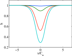
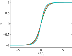
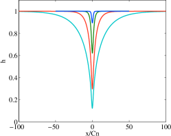
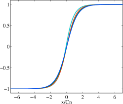
Figure 4: Solutions of the thin-film equations obtained by solving the boundary-value problem (39b). Across the top: the effect on the equilibrium solutions of varying the backreaction strength, for parameter values $C=C_{\mathrm{n}}^{2}G=1$ and $r=0.1,1,10,50$. In (a) the valley deepens with increasing $r$ although the film never ruptures, while in (b) the front steepens with increasing $r$. Figs. (a) and (b) are taken from Ó Náraigh and Thiffeault ONaraigh2007 . Across the bottom: the effect on the equilibrium solutions of varying the strength of the regularizing potential. The parameter values are $C=C_{\mathrm{n}}^{2}=r=1$ and $G=0.001,0.01,0.1,1$. In (c) the valley deepens with decreasing $G$ although the film never ruptures, while in (d) the front steepens with decreasing $G$.

The repulsive Van der Waals potential therefore has a regularizing effect on the solutions. Indeed, the formation of the valley in the height field has the physical interpretation of a balance between the Van der Waals and backreaction effects. From Fig. 5

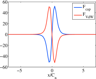
Figure 5: Boundary-value solution. A plot of the forces $F_{\mathrm{cap}}$ and $F_{\mathrm{vdW}}$ for $C=C_{\mathrm{n}}^{2}=G=1$ and $r=50$: they have opposite sign; hence, the regularizing potential opposes the rupture-inducing tendency of the backreaction.

we see that the backreaction force, which, through Eq. (21d) we identify as $F_{\mathrm{cap}}=-rh^{-1}\partial_{x}\left[h\left(\partial_{x}c\right)^{2}\right]$, is of opposite sign to the Van der Waals force $F_{\mathrm{VdW}}=G\partial_{x}h^{-3}$. Now in Sec. III we showed how the Van der Waals force inhibits rupture; hence, $F_{\mathrm{cap}}$ must promote it. The depth of the valley in the height field is therefore selected through a balance between rupture-preventing and rupture-promoting effects.

Finally, we compare the results for the minimum free-surface height implied by the solution of the boundary value problem (BVP) with the theoretical lower bound obtained in Sec. III. In terms of the physical parameters of the system, the no-rupture condition of Sec. III is

$$h_{\mathrm{min}}\geq s_{*}=\sqrt{2CL(F_{0}+F_{1}G)}\left(\sqrt{\frac{e^{4CG^{-1}\left(F_{0}+F_{1}G\right)^{2}}}{e^{4CG^{-1}\left(F_{0}+F_{1}G\right)^{2}}-1}}-1\right)>0,$$

where $F_{1}=\tfrac{1}{2}\int_{\Omega}{dx}\left[h\left(x,0\right)\right]^{-2}\neq 0$, and $F_{0}=\mathcal{F}\left(0\right)-F_{1}$. The function $s_{*}\left(G,C\right)$ has no explicit $r$-dependence: although $F_{0}$ depends on $r$, it is possible to find initial data to remove this dependence. We show a representative plot of $s_{*}\left(G,C\right)$ in Fig. 6 (a), while in (b) we show a plot of $h_{\mathrm{min}}$ as a function of $G$, obtained from the solution of the BVP. Now although these two figures represent solutions to the model equations for different boundary conditions, a comparison between them is warranted, especially at a domain boundary, where the film thinning is induced by entirely local effects. The shape of the two bounds in Figs. 6 (a) and (b) is different. Since the bound in Fig. 6 (b) is obtained from numerical simulations, and is intuitively correct, we conclude that it has the correct shape and that the bound of Fig. 6, while mathematically indispensable, is not sharp enough to be useful in determining the parametric dependence of the dip in free-surface height.

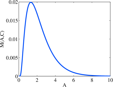
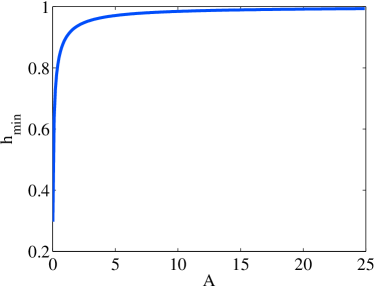
Figure 6: (a) A typical plot of $s_{*}\left(G,C\right)$ for $F_{0}=F_{1}=\tfrac{1}{2}$ and $C=1$. This theoretical lower bound has a different shape from that in (b), which is obtained from a solution of the BVP, with $C=r=1$. This suggests that while $s_{*}\left(G,C\right)$ plays an important role in the analysis of the model equations, it does not capture the physics of film thinning.

IV.2 Numerical studies without a regularizing Van der Waals potential: a study of rupture

We perform numerical simulations of the full equations (21d), with the following finite-amplitude initial data:

$$h\left(x,0\right)=1+0.1\sin\left[3\left(2\pi/L\right)x+\pi\right],\qquad c\left(x,0\right)=0.5\sin\left[3\left(2\pi/L\right)x\right].$$

We use the parameters $r=2$, $G=0$, $C=1$, $C_{\mathrm{n}}=0.1$, and $L=2\pi$. The calculations are carried out on a periodic domain, with $512$, and $1024$ gridpoints and a timestep $\Delta t=10^{-6}$. The regularizing Van der Waals force is no longer present, and thus the estimates of Sec. III no longer apply. We therefore examine the possibility that the film will rupture in finite time. For the parameter values chosen, rupture does indeed occur in finite time, as evidenced by Fig. 7.

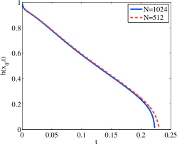
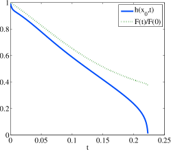
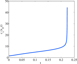
Figure 7: (a) Temporal evolution of the minimum free-surface height. The rupture is hastened by grid refinement; (b) our numerical simulation also captures the decay of the free energy; (c) the rupture coincides with a finite-time singularity, wherein the derivative $c_{x}$ diverges at the point where $h$ touches down.

In the numerical simulation, rupture is only hastened by grid refinement: this indicates that the effect does not disappear with an increase in resolution, but is nevertheless difficult to capture precisely. The simulation also decreases the free energy. This is consistent with the free-energy decay law derived in Sec. III, which relies only on the fact that $h$ should be positive, and holds even for zero Van der Waals forces. Thus, we are satisfied that the rupture is accurately described by the numerical simulation, and is not simply an artefact.

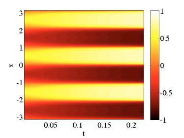
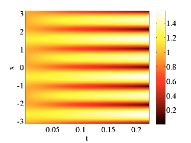
Figure 8: No regularizing potential and large backreaction effect, $r=2$. Temporal evolution of (a) the concentration; (b) the free-surface height. The height touches down to zero in finite time. A singularity develops in the equations and the gradient of the concentration diverges in the transition zone.

The evolution towards rupture is shown again in Fig. 8. The figure demonstrates yet again that rupture is induced in the transition zones of concentration. Our understanding of rupture is strengthened by a further examination of the equilibrium case described by Eqs. (39b). For $G=0$, the $h$-equation reads

$$\frac{1}{C}\frac{\partial^{2}h}{\partial x^{2}}=r\left[\tfrac{1}{4}\left(c^{2}-1\right)^{2}+\tfrac{1}{2}\left(\frac{\partial{c}}{\partial{x}}\right)^{2}\right].$$ (43)

As a boundary-value problem, with boundary conditions $h=1$ as $x\rightarrow\pm\infty$ and $c=\pm 1$, $c_{x}=0$ as $x\rightarrow\pm\infty$, Eq. (43) has no solution, since $h_{xx}>0$ everywhere is not compatible with a bounded solution. In the language of dynamical systems, the proposed boundary conditions for the solution pair $\left(h,h_{x}\right)$ imply a homoclinic orbit, which is impossible if $h_{xx}$ is positive everywhere. Thus, the development of a finite-time singularity is consistent with the non-existence of a time-independent solution of the $\left(h,c\right)$ equation pair.

Our numerical study has demonstrated the sharp difference in the two cases wherein the repulsive Van der Waals force is either included or neglected. In the case where this force is neglected, the film ruptures in finite time, an event that is accompanied by the development of a singularity in the derivative in the concentration. While interesting mathematically, this is undesirable from a physical point of view. Consistent with the analysis of Sec. III, the inclusion of the Van der Waals term prevents rupture, and enables the development of an equilibrium state. Note finally that simulations involving two lateral directions have elsewhere been carried out by the authors ONaraigh2007 , and the qualitative features are similar to those obtained here.

V Conclusions

Starting from the Navier–Stokes Cahn–Hilliard equations, we have derived a pair of nonlinear parabolic PDEs that describe the coupled effects of phase separation and free-surface variations in a thin film of binary liquid. Since we are interested in the long-time outcome of the phase separation, we have focussed on liquids that experience a repulsive Van der Waals force, which tends to inhibit film rupture. Using physical intuition, we identified a decaying energy functional that facilitated analysis of the equations. Based on this decaying energy functional, we have developed a series of a priori estimates for positive solutions $\left(h,c\right)$, $h>0$ to the model equations (21d). The Hölder continuity of $h$ obtained through the decaying energy gives rise to a positive lower bound on the height $h$, valid for a general family of repulsive potentials. These estimates are valid not only in the a priori sense described here, but also as a means of demonstrating the existence of regular solutions to Eqs. (21d), given appropriate initial data Friedman1990 ; ONaraighPhD .

We carried out one-dimensional numerical simulations of the equations (21d) and found that the free-surface height and concentration tend to an equilibrium state. The concentration forms domains; that is, extended regions where $c\approx\pm 1$. The domains are separated by narrow zones where the concentration smoothly transitions between the limiting values $\pm 1$. At the transition zones, the free surface dips below its mean value to form a ‘valley’, a feature of binary thin-film behaviour that is observed in experiments. To study the valley depth as a function of the problem parameters, we focussed on solving the equilibrium version of Eq. (21d) as a boundary-value problem. This simplification is carried out without much loss of generality, since our numerical simulations indicate that the system tends asymptotically to such a state. We have shown that the valley becomes shallower upon increasing the strength of the repulsive Van der Waals force, while it deepens when the backreaction strength is increased. The film-thinning tendency of the backreaction has been observed experimentally WangH2000 ; WangW2003 ; ChungH2004 . In the limit of zero repulsive Van der Waals forces, the solution of the boundary-value problem implies that the film ruptures, and our temporal numerical simulations confirm this. Indeed, we have demonstrated that the film ruptures in finite time; simultaneously, the derivative of the concentration becomes singular. Since such singularities are undesirable from a physical point of view, this result underscores the importance of including Van der Waals forces in studies like this one.

Acknowledgements. We thank G. Pavliotis for helpful discussions. L.Ó.N. was supported by the Irish government and the UK Engineering and Physical Sciences Research Council.

Appendix A

In this section we outline a numerical technique for the equations

$$\frac{\partial h}{\partial t}+\frac{\partial}{\partial x}\left(hu\right)=0,\qquad\frac{\partial c}{\partial t}+u\frac{\partial c}{\partial x}=\frac{1}{h}\frac{\partial}{\partial{x}}\left(h\frac{\partial\mu}{\partial{x}}\right),$$ (44a)

where

$$u=-\tfrac{1}{3}h^{2}\bigg{\{}\frac{\partial}{\partial{x}}\left(-\frac{1}{C}\frac{\partial^{2}{h}}{\partial{x}^{2}}+\phi\right)+\frac{r}{h}\frac{\partial}{\partial{x}}\left[h{\left(\frac{\partial{c}}{\partial{x}}\right)}^{2}\right]\bigg{\}},$$ (44b)

$$\mu=c^{3}-c-\frac{C_{\mathrm{n}}^{2}}{h}\frac{\partial}{\partial{x}}\left(h\frac{\partial{c}}{\partial{x}}\right).$$ (44c)

We impose periodic boundary conditions on the solution $\left(h,c\right)$ and its derivatives. The solution $\left(h,c\right)$ is discretized on a regular spatial grid such that the vector pair $\left(\bm{h}\left(t\right),\bm{c}\left(t\right)\right)\in\mathbb{R}^{N}\times\mathbb{R}^{N}$ represents the discretized solution at time $t$. The derivatives are approximated as centred finite differences with the periodic boundary conditions taken into account. Thus, the derivatives are reduced to matrix operators $\mathcal{D}_{j}$ on $\mathbb{R}^{N}$ (here the subscript ‘$j$’ denotes the order of the derivative). The solution is marched forwards in time using a semi-implicit Euler algorithm,

$$\frac{\bm{h}^{n+1}-\bm{h}^{n}}{\Delta t} = -\frac{1}{3C}\mathcal{D}_{1}\left[\left(\bm{h}^{n}\right)^{\cdot 3}\cdot\left(\mathcal{D}_{3}\bm{h}^{n+1}\right)\right]+\bm{S}_{h}^{n},$$

$$\frac{\bm{c}^{n+1}-\bm{c}^{n}}{\Delta t} = -C_{\mathrm{n}}^{2}\left[\mathcal{D}_{4}\bm{c}^{n+1}\right]+\bm{S}_{c}^{n},$$ (45)

where the ‘dot’ is used here to denote pointwise multiplication, $\bm{x}\cdot\bm{y}=\left(x_{1}y_{1},\cdots,x_{N}y_{N}\right)$, $\bm{x}^{\cdot a}=\left(x_{1}^{a},\cdots,x_{N}^{a}\right)$, and where the ‘source’ terms $\bm{S}_{h}$ and $\bm{S}_{c}$ are defined as follows:

$$\bm{S}_{h} = \tfrac{1}{3}\mathcal{D}_{1}\bigg{\{}\left(\bm{h}^{\cdot 3}\right)\cdot\bigg{[}\mathcal{D}_{1}\bm{\phi}+r\left(\bm{h}^{\cdot-1}\right)\cdot\left[\mathcal{D}_{1}\left(\bm{h}\cdot\left(\mathcal{D}_{1}\bm{c}\right)^{\cdot 2}\right)\right]\bigg{]}\bigg{\}},$$

$$\bm{S}_{c} = -\bm{u}\cdot\left(\mathcal{D}_{1}\bm{c}\right)+\left(\bm{h}^{\cdot-1}\right)\cdot\left(\mathcal{D}_{1}\bm{h}\right)\cdot\left(\mathcal{D}_{1}\bm{\mu}\right)+\mathcal{D}_{2}\left[\bm{c}^{\cdot 3}-\bm{c}-C_{\mathrm{n}}^{2}\left(\bm{h}^{\cdot-1}\right)\cdot\left(\mathcal{D}_{1}\bm{h}\right)\cdot\left(\mathcal{D}_{1}\bm{c}\right)\right],$$

$$\bm{u} = -\tfrac{1}{3}\left(\bm{h}^{\cdot 2}\right)\cdot\bigg{[}-\frac{1}{C}\mathcal{D}_{3}\bm{h}+\mathcal{D}_{1}\bm{\phi}+r\left(\bm{h}^{\cdot-1}\right)\cdot\left[\mathcal{D}_{1}\left(\bm{h}\cdot\left(\mathcal{D}_{1}\bm{c}\right)^{\cdot 2}\right)\right]\bigg{]},$$

$$\bm{\mu} = \bm{c}^{\cdot 3}-\bm{c}-C_{\mathrm{n}}^{2}\left(\bm{h}^{\cdot-1}\right)\cdot\left(\mathcal{D}_{1}\bm{h}\right)\cdot\left(\mathcal{D}_{1}\bm{c}\right)-C_{\mathrm{n}}^{2}\mathcal{D}_{2}\bm{c}.$$ (46)

Equations (45) are re-written as

$$\left[\bm{1}+\frac{\Delta t}{3C}\mathcal{D}_{1}\left(\left(\bm{h}^{n}\right)^{\cdot 3}\cdot\mathcal{D}_{3}\right)\right]\bm{h}^{n+1} = \bm{h}^{n}+\Delta t\,\bm{S}_{h}^{n},$$ (47)

$$\left[\bm{1}+\Delta tC_{\mathrm{n}}^{2}\mathcal{D}_{4}\right]\bm{c}^{n+1} = \bm{c}^{n}+\Delta t\,\bm{S}_{c}^{n},$$ (48)

a linear problem that is solvable for $\left(\bm{h}^{n+1},\bm{c}^{n+1}\right)$ by matrix inversion. The $\bm{h}$-equation manifestly conserves the sum $\sum_{i=1}^{N}h_{i}$, since $\sum_{i=1}^{N}\sum_{j=1}^{N}\mathcal{D}_{1,ij}v_{j}=0$, for any vector $\bm{v}\in\mathbb{R}^{N}$. Other semi-implicit numerical schemes

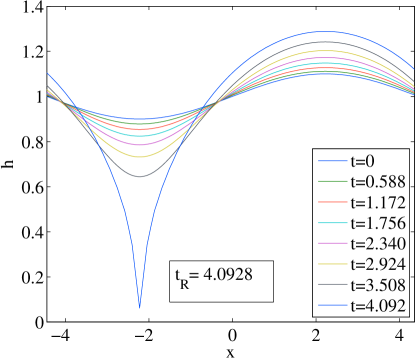
Figure 9: Comparison with the work of Burelbach et al. for the rupture of a single-component fluid under the influence of an attractive Van der Waals potential. The rupture happens in finite time and is calculated here as $t_{R}=4.093$, for simulation parameters $\Delta t=10^{-5}$ and $N=100$.

that only approximate this conservation law can fail near rupture ($h\rightarrow 0$). One such technique is the otherwise successful method of Kondic Kondic2003 , which replaces the term $\left(\bm{h}^{n}\right)^{\cdot 3}\cdot\left(\mathcal{D}_{3}\bm{h}^{n+1}\right)$ with $\left(\bm{h}^{n+1}\right)^{\cdot 3}\cdot\left(\mathcal{D}_{3}\bm{h}^{n+1}\right)$ and thus involves a Newton iteration at each timestep.

Now although the implied conservation law $\partial_{t}\int_{0}^{L}ch\,dx$ is not manifest in the $\bm{c}$-equation (48), we have verified that a sufficiently small stepsize and gridsize guarantees its conservation in practice. The implicit step in Eq. (48) is particularly fast because the matrix $1+\Delta tC_{\mathrm{n}}^{2}\mathcal{D}_{4}$ need only be inverted once. This implicit treatment of the high-order derivatives in Eqs. (47)–(48) also ensures numerical stability for large timesteps that would otherwise cause numerical blowup.

We verify the correctness of our numerical scheme by comparing it against a set of well-known results for the single-component equation

$$h_{t}+\left(h^{-1}h_{x}\right)_{x}+\left(h^{3}h_{xxx}\right)_{x}=0,$$

which touches down to zero in finite time. This equation has been studied by Burelbach et al. Burelbach1988 , with the initial condition

$$h_{0}=1+0.1\sin\left(x/\sqrt{2}\right).$$

They observed finite-time rupture and estimated the the rupture time as $t_{R}=4.164$, based on a numerical study with $\Delta t=10^{-5}$ and $N=40$. With these grid parameters, the numerical scheme (47)–(48) gives a rupture time $t_{R}=4.145$. A possible source for the small discrepancy of estimates is the fact that we have kept $\Delta t=10^{-5}$ for the duration of the simulation; Burelbach et al. refine it as rupture approaches, until $\Delta t=10^{-5}$. Refining the grid ($N=100$) gives a reduced rupture time $t_{R}=4.093$ (see Fig. 9), a reduction that is consistent with Fig. 3 of Burelbach et al. In conclusion, this test of our scheme validates its applicability to the two-component equations (44c).

References

- (1) J. W. Cahn and J. E. Hilliard. Free energy of a nonuniform system. I. Interfacial energy. J. Chem. Phys, 28:258–267, 1957.
- (2) A. J. Bray. Theory of phase-ordering kinetics. Adv. Phys., 43:357–459, 1994.
- (3) K. R. Elder, T. M. Rogers, and R. C. Desai. Early stages of spinodal decomposition for the Cahn–Hilliard–Cook model of phase separation. Phys. Rev. B, 38:4725, 1988.
- (4) J. Zhu, L. Q. Shen, J. Shen, V. Tikare, and A. Onuki. Coarsening kinetics from a variable mobility Cahn–Hilliard equation: Application of a semi-implicit Fourier spectral method. Phys. Rev. E, 60:3564–3572, 1999.
- (5) L. Ó Náraigh and J.-L. Thiffeault. Bubbles and Filaments: Stirring a Cahn–Hilliard Fluid. Phys. Rev. E, 75:016216, 2007.
- (6) D. G. A. L. Aarts, R. P. A. Dullens, and H. N. W. Lekkerherker. Interfacial dynamics in demixing systems with ultralow interfacial tension. New J. Phys., 7:14, 2005.
- (7) H. Ding, P. D. M. Spelt, and C. Shu. Diffuse interface model for incompressible two-phase flows with large density ratios. J. Comp. Phys., 226:2078, 2007.
- (8) J. Lowengrub and L. Truskinowsky. Quasi-incompressible Cahn–Hilliard fluids and topological transitions. Proc. R. Soc. Lond. A, 454:2617–2654, 1998.
- (9) D. S. Cohen and J. D. Murray. A generalized diffusion model for growth and dispersal in a population. J. Math. Biology, 12:237, 1981.
- (10) C. M. Elliott and S. Zheng. On the Cahn–Hilliard equation. Arch. Rat. Mech. Anal., 96:339–357, 1986.
- (11) C. M. Elliott and H. Garcke. The Cahn–Hilliard equation with degenerate mobility. SIAM J. Math. Anal., 27:403–423, 1996.
- (12) H. Gajewski and K. Zacharias. On a nonlocal phase separation model. J. Math. Anal. Appl., 286:11–31, 2003.
- (13) S. Berti, G. Boffetta, M. Cencini, and A. Vulpiani. Turbulence and coarsening in active and passive binary mixtures. Phys. Rev. Lett., 95:224501, 2005.
- (14) L. Berthier, J. L. Barrat, and J. Kurchan. Phase separation in a chaotic flow. Phys. Rev. Lett., 86:2014–2017, 2001.
- (15) A. M. Lacasta, J. M. Sancho, and F. Sagues. Phase separation dynamics under stirring. Phys. Rev. Lett., 75:1791, 1995.
- (16) A. Oron, S. H. Davis, and S. G. Bankoff. Long-scale evolution of thin liquid films. Rev. Mod. Phys., 69:931, 1997.
- (17) R. V. Craster and O. K. Matar. Dynamics and stability of thin liquid films. Rev. Mod. Phys., 81:1131, 2009.
- (18) L. Ó Náraigh and J.-L. Thiffeault. Dynamical effects and phase separation in cooled binary fluid films. Phys. Rev. E, 76:035303(R), 2007.
- (19) A. Karim, J. F. Douglas, L. P. Sung, and B. D. Ermi. Self-assembly by phase separation in polymer thin films. Encyclopedia of Materials: Science and Technology, page 8319, 2002.
- (20) K. Mertens, V. Putkaradze, D. Xia, and S. R. Brueck. Theory and experiment for one-dimensional directed self-assembly of nanoparticles. J. App. Phys., 98:034309, 2005.
- (21) D. Kim and W. Lu. Interface instability and nanostructure patterning. Comp. Mater. Sci., 38(2):418–425, 2006.
- (22) D. Xia and S. Brueck. A facile approach to directed assembly of patterns of nanoparticles using interference lithography and spin coating. Nano Letters, 4:1295, 2004.
- (23) G. Krausch, E. J. Kramer, M. H. Rafailovich, and J. Sokolov. Self-assembly of a homopolymer mixture via phase separation. Appl. Phys. Lett., 64:2655, 1994.
- (24) W. Lu and D. Salac. Patterning multilayers of molecules via self-organization. Phys. Rev. Lett., 94:146103, 2005.
- (25) D. D. Holm and V. Putkaradze. Aggregation of finite size particles with variable mobility. Phys. Rev. Lett., 95:226106, 2005.
- (26) F. Bernis and A. Friedman. Higher order nonlinear degenerate parabolic equations. J. Differential Equations, 83:179–206, 1990.
- (27) T. G. Myers. Thin films with high surface tension. SIAM Review, 40:441, 1998.
- (28) A. L. Bertozzi and M. C. Pugh. The lubrication approximation for thin viscous films: regularity and long-time behaviour of weak solultions. Comm. Pure Appl. Math., XLIX:85, 1996.
- (29) A. L. Bertozzi and M. C. Pugh. Long-wave instabilities and saturation in thin film equations. Comm. Pure Appl. Math., LI:0625, 1998.
- (30) R. S. Laugesen and M. C. Pugh. Heteroclinic orbits, mobility parameters and stability for thin film type equations. J. Differential Equations, 95:1–29, 2002.
- (31) S. Wieland and H. Garcke. Surfactant spreading on thin viscous films: Nonnegative solutions of a coupled degenerate system. SIAM J. Math. Anal., 37:2025, 2006.
- (32) O. A. Frolovskaya, A. A. Nepomnyashchy, A. Oron, and A. A. Golovin. Stability of a two-layer binary-fluid system with a diffuse interface. Phys. Fluids, 20:112105, 2009.
- (33) L. Sung, A. Karim, J. F. Douglas, and C. C. Han. Dimensional crossover in the phase separation kinetics of thin polymer blend films. Phys. Rev. Lett., 76:4368, 1996.
- (34) G. Grün and M. Rumpf. Simulation of singularities and instabilities arising in thin film flow. Euro. Jnl. of Applied Mathematics, 12:293, 2001.
- (35) L. Ó Náraigh. The role of advection in phase-separating binary liquids. PhD thesis, Imperial College London, 2008. Eprint: arXiv:0805.1242v1.
- (36) H. Wang and R. J. Composto. Thin film polymer blends undergoing phase separation and wetting: identification of early, intermediate, and late stages. J. Chem. Phys., 113:10386, 2000.
- (37) W. Wang, T. Shiwaku, and T. Hashimoto. Phase separation dynamics and pattern formation in thin films of a liquid crystalline copolyester in its biphasic region. Macromolecules, 36:8088, 2003.
- (38) H. Chung and R. J. Composto. Breakdown of dynamic scaling in thin film binary liquids undergoing phase separation. Phys. Rev. Lett., 92:185704–1, 2004.
- (39) L. Kondic. Instabilities in gravity driven flow of thin fluid films. SIAM Review, page 95, 2003.
- (40) J. P. Burelbach, S. G. Bankoff, and S. H. Davis. Nonlinear stability of evaporating / condensing liquid films. J. Fluid Mech., 195:463, 1988.