Holographic calculation of hadronic contributions to muon $g-2$

Abstract

Using the gauge/gravity duality, we compute the leading order hadronic (HLO) contribution to the anomalous magnetic moment of muon, $a_{\mu}^{\rm HLO}$. Holographic renormalization is used to obtain a finite vacuum polarization. We find $a_{\mu}^{\rm HLO}=470.5\times 10^{-10}$ in AdS/QCD with two light flavors, which is compared with the currently revised BABAR data estimated from $e^{+}e^{-}\to\pi^{+}\pi^{-}$ events, $a_{\mu}^{\rm HLO}[\pi\pi]=(514.1\pm 3.8)\times 10^{-10}$.

I Introduction

A recent high-precision measurement of $\pi^{+}\pi^{-}$ cross section by the BABAR experiment Aubert:2009fg has found that the previous $e^{+}e^{-}$-based evaluation of the leading hadronic (HLO) contributions to muon $g-2$ was fairly underestimated. With this new measurement the discrepancy between the $e^{+}e^{-}$ and $\tau$-based results for the dominant two-pion mode is narrowed to $1.5\,\sigma$ level in the dispersion integral Davier:2009zi . It is therefore quite necessary to find other means to test this new experimental data.

To confirm the new BABAR data one needs to calculate it directly from QCD, for which Lattice QCD would certainly be the best tool. However, the state-of-the-art calculations of lattice QCD still suffer from a large systematic error, compared to the experimental value, due to difficulties in simulating light quarks Blum:2009zz .

There have been a few other attempts to calculate the HLO contribution from QCD, using chiral perturbation or $1/N_{c}$ expansion, or from models of QCD such as the extended Nambu-Jona-Lasinio models deRafael:1993za or the quark resonance model Pallante:1994ee . In this paper we use recently proposed models of QCD, called holographic QCD Erlich:2005qh ; Da Rold:2005zs ; Hong:2006ta ; Sakai:2004cn , based on the gauge/gravity duality, to calculate the hadronic vacuum polarization contribution. The holographic models of QCD were found to be quite successful to account for the properties of hadrons at low energy and give relations to their couplings and also new sum rules Hong:2007kx . Similar attempt was made recently to estimate successfully the hadronic light-by-light contribution to the anomalous magnetic moment of muon Hong:2009zw .

II General formulas and AdS/QCD

Hadrons (or quarks) contribute to the anomalous magnetic moment of muon only through quantum fluctuations. The leading contribution is therefore the vacuum polarization correction, shown in Fig. 1, to the internal photon line, $\Pi_{\rm em}^{\rm had}(Q^{2})$, which is defined in QCD by the electromagnetic currents of quarks, $J_{\rm em}^{\mu}=\sum_{f}\bar{q}_{f}\gamma^{\mu}Q_{\rm em}q_{f}$ $(f=u,d,s,\cdots)$ with the electric charge operator $Q_{\rm em}$ , as

$$i\int d^{4}x\,e^{iqx}\langle 0|TJ_{\rm em}^{\mu}(x)J_{\rm em}^{\nu}(0)|0\rangle=(q^{2}\eta^{\mu\nu}-q^{\mu}q^{\nu})\Pi_{\rm em}^{\rm had}(-q^{2})\,,$$ (1)

where $\eta^{\mu\nu}={\rm diag}(1,-1,-1,-1)$. Since the (bare) vacuum polarization function is a divergent quantity, one should regularize it with a regulator and renormalize it by adding a counterterm. Furthermore, if one uses the physical charge in the calculation of muon $g-2$, the renormalized vacuum function should be modified as

$$\bar{\Pi}_{\rm em}^{\rm had}(Q^{2})=\Pi_{\rm em}^{\rm had}(Q^{2})-\Pi_{\rm em}^{\rm had}(0)$$ (2)

so that the pole residue of the photon propagator does not get shifted.

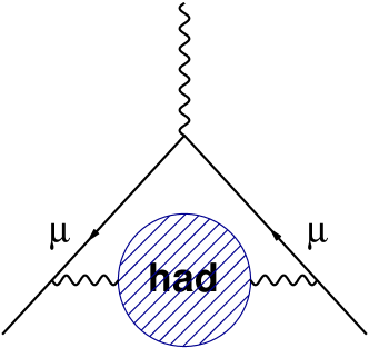
Figure 1: Leading hadronic-vacuum-polarization contribution to muon $g-2$.

After the vacuum polarization function is obtained, we can calculate the hadronic leading order correction to the anomalous magnetic moment of muon, using the formula derived in Blum:2002ii ; Aubin:2006xv  

$$a_{\mu}^{\rm HLO}=4\pi^{2}\left(\frac{\alpha}{\pi}\right)^{2}\int_{0}^{\infty}dQ^{2}f(Q^{2})\,\bar{\Pi}_{\rm em}^{\rm had}(Q^{2})\,,$$ (3)

where $Q^{2}$ is the Euclidean momentum-squared and the kernel is given as

$$f(Q^{2})=\frac{m_{\mu}^{2}Q^{2}Z^{3}(1-Q^{2}Z)}{1+m_{\mu}^{2}Q^{2}Z^{2}}\quad{\rm with}\;\;Z=-\frac{Q^{2}-\sqrt{Q^{4}+4m_{\mu}^{2}Q^{2}}}{2m_{\mu}^{2}Q^{2}}\,.$$ (4)

It is straightforward in holographic QCD to calculate the correlation functions of QCD flavor currents. According to the gauge/gravity duality, the classical gravity action of holographic dual becomes the generating functional for the one-particle irreducible (1PI) functions of the boundary gauge theory in the large $N_{c}$ limit, and the bulk fields, evaluated at the UV boundary, serve as sources for the currents. Though the exact duality has not been established for QCD yet, as a simple model, we consider a holographic model of QCD, proposed by Erlich et al. Erlich:2005qh for the calculation of the muon anomalous magnetic moment. Our analysis, however, can be easily applied to other holographic models such as Sakai-Sugimoto model Sakai:2004cn  

The AdS/QCD action Erlich:2005qh , relevant to our present computation, is given in a slice of five dimensional anti de Sitter (AdS) space of unit radius as

$$S_{\rm AdS/QCD}[L,R,X]=\int d^{4}x\int_{\epsilon}^{z_{m}}dz\,\sqrt{g}\,{\rm Tr}\left[-\frac{1}{4g_{5}^{2}}(F_{R}^{2}+F_{L}^{2})+|DX|^{2}+3|X|^{2}\right]\,,$$ (5)

where $g={\rm det}[g_{MN}]$, $g_{MN}=(1/z)^{2}\eta_{MN}$ with $\eta_{MN}={\rm diag}(1,-1,-1,-1,-1)$, $F_{R,L}\equiv\partial_{M}R(L)_{N}-\partial_{N}R(L)_{M}-i[R(L)_{M},R(L)_{N}]$ with the gauge fields $L_{M},R_{M}$ of the ${\rm U}(N_{f})_{L}\times{\rm U}(N_{f})_{R}$ gauged-flavor symmetry in the 5D bulk and $X$ denotes the bulk scalar fields, transforming under the gauge symmetry as $X\to U_{L}XU_{R}^{\dagger}$. One could add higher dimensional operators in the AdS/QCD action (5) such as $|X|^{2}\,F^{2}$ or $F^{4}$, but they are suppressed by $\alpha^{\prime}$ and thus negligible at low energy. The bulk scalar gets a vacuum expectation value to break the bulk gauge symmetry down to its vectorial subgroup ${\rm U}(N_{f})$,

$$\left\langle X\right\rangle=\frac{1}{2}{M}\,z+\frac{1}{2}{\Sigma}\,z^{3}$$ (6)

where ${M}={\rm diag}(m_{u},m_{d},m_{s},\cdots)$ is the current quark mass matrix and $\Sigma$ is the chiral condensate.

Introducing the vector and axial vector gauge fields, $V=(L-R)/{2}$ and $A=(L+R)/{2}$, respectively, and working in $V_{z}=A_{z}=0$ gauge, we can derive the equations of motion for $V_{\mu}$ and $A_{\mu}$ and solve them by imposing the boundary conditions for $V_{\mu}$ and $A_{\mu}$ as well as for the bulk scalar field $X$, following the familiar AdS/CFT dictionary. One should note, however, that as far as the large-$N_{c}$ contributions (equivalently the meson exchanges at tree-level) to the vector-current correlator $\Pi_{V}(Q^{2})$ are concerned, we are allowed to focus only on (infinite tower of) neutral vector mesons coupled to the vector currents as illustrated in Fig. 2. The values of vector meson decay constants and their masses are calculable in holographic QCD.

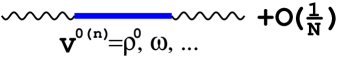
Figure 2: A diagram illustrating neutral vector meson exchanges giving dominant contributions to $\Pi_{V}$ at the large $N_{c}$ limit.

Since the electromagnetic charge $Q_{\rm em}=\frac{1}{3}T_{0}+T_{3}$ in the case of two flavors, where the generators of flavor symmetry $T_{0}=\frac{1}{2}{\bf 1}_{2\times 2}$ and $T_{3}={\rm diag}(\frac{1}{2},-\frac{1}{2})$ , the quark electromagnetic currents are given as

$$J_{\rm em}^{N_{f}=2}=\frac{1}{3}J_{0}+J_{3}\,.$$ (7)

In the limit of exact flavor symmetry the vector-current correlator is given as

$$i\int d^{4}xe^{iqx}\langle 0|TJ_{V}^{a\mu}(x)J_{V}^{b\nu}(0)|0\rangle=\delta^{ab}(q^{2}\eta^{\mu\nu}-q^{\mu}q^{\nu})\Pi_{V}(-q^{2})\,,$$ (8)

with $a,b$ being indices of the ${\rm U}(2)$ flavor symmetry. We have then

$$\Pi_{\rm em}^{N_{f}=2}(-q^{2})=\frac{10}{9}\Pi_{V}(-q^{2})\,.$$ (9)

For $N_{f}=3$ we have $J_{\rm em}^{N_{f}=3}=J_{3}+\frac{1}{\sqrt{3}}J_{8}$ and $\Pi_{\rm em}^{N_{f}=3}(-q^{2})=\frac{4}{3}\Pi_{V}(-q^{2})$ in the exact limit of the ${\rm U}(3)$ flavor symmetry.

III Holographic Vacuum Polarization

Since we are interested in two-point functions of flavor currents, we need to keep terms quadratic in the bulk gauge fields for a given vacuum solution for $\left<X\right>$ in the action (5). If we neglect the higher order terms like $|X|^{2}F^{2}$, the vector gauge fields do not couple to the chiral condensate $\Sigma$ but may couple to the current quark mass operator, $M$. However, at the leading order, the neutral vectors do not couple to $X$ at all and have same mass among them, since $[V_{\mu}^{0},\left\langle X\right\rangle]=0$.

The equations for vectors are given at the leading order as

$$\left(\partial_{z}\frac{1}{z}\partial_{z}+\frac{q^{2}}{z}\right)V_{\perp\mu}^{a}(q,z)=0\,,$$ (10)

where $V_{\perp\mu}^{a}(q,z)=v_{\mu}^{a}(q)V_{\perp}(q,z)$ is the transverse component of the Fourier transform of the vector field $V_{\mu}(x,z)=V_{\mu}^{a}(x,z)T^{a}$. Imposing the boundary condition $\partial_{z}V^{a}_{\mu}(q,z_{m})=0$ and $V^{a}_{\mu}(q,\epsilon)=v_{\mu}^{a}(q)$, one gets the solution to Eq. (10) given by Bessel functions. Putting the solution into the action, we are left with the boundary action Erlich:2005qh ,

$$S_{\rm eff}[v_{\mu}]=-\frac{1}{2}\int\frac{d^{4}q}{(2\pi)^{4}}v_{\mu}^{a}(-q)\left[\frac{1}{g_{5}^{2}}\frac{V_{\perp}(q,z)\partial_{z}V_{\perp}(q,z)}{z}\right]_{z=\epsilon}v^{\mu a}(q)\,,$$ (11)

which becomes the generating functional for the 1PI correlation functions of the QCD flavor currents, $W^{\rm QCD}_{\rm 4D}[v_{\mu}]\equiv S_{\rm eff}[v_{\mu}]$ .

From Eq. (8) we immediately read off the transverse part of the vector current two-point functions,

$$\frac{\delta^{2}S_{\rm eff}[v_{\mu}]}{\delta v^{\mu a}(-q)\delta v^{\nu b}(q)}=i\int d^{4}xe^{iqx}\langle 0|TJ_{V}^{a\mu}(x)J_{V}^{b\nu}(0)|0\rangle_{\perp}\,.$$ (12)

Using Eq. (12) and the action (11), we find the vector current correlator $\Pi_{V}(q^{2})$ in terms of the five dimensional gravity dual,

$$\Pi_{V}(q^{2}) = -\frac{1}{g_{5}^{2}}\left[\frac{\partial_{z}V_{\perp}(q,z)}{q^{2}\,z}\right]_{z=\epsilon}$$ (13)

$$= -\frac{1}{g_{5}^{2}}\frac{1}{q\epsilon}\frac{J_{0}(qz_{m})Y_{0}(q\epsilon)-Y_{0}(qz_{m})J_{0}(q\epsilon)}{J_{0}(qz_{m})Y_{1}(q\epsilon)-Y_{0}(qz_{m})J_{1}(q\epsilon)}\,.$$

Note that this $\Pi_{V}(q^{2})$ behaves like $\ln\epsilon$ as the UV cutoff $\epsilon\to 0$, so it needs to be renormalized. To make this point clearer, we may expand Eq. (13) perturbatively in power of $\epsilon$ to obtain the asymptotic form of $\Pi_{V}(q^{2})$,

$$\Pi_{V}(q^{2})=\frac{1}{g_{5}^{2}}\left[-\frac{\pi}{2}\frac{Y_{0}(qz_{m})}{J_{0}(qz_{m})}+\gamma-\ln 2+\ln q\epsilon+{\cal O}(\epsilon^{2})\right]\,,$$ (14)

where $\gamma$ is the Euler constant. In order to renormalize the vacuum polarization function, we shall adopt a procedure of the holographic renormalization Bianchi:2001kw ; Skenderis:2002wp , which is appropriate in our holographic approach. The holographic renormalization can be performed by introducing a counterterm at the UV boundary, respecting all the residual 4d-gauge symmetry, which subtracts only the divergent term in the vacuum polarization (14), just like the familiar minimal subtraction scheme. We find the counterterm appropriate to renormalize $\Pi_{V}(q^{2})$,

$$S_{\rm c}(\mu)=\int d^{4}x\left(\frac{1}{2g_{5}^{2}}\ln\epsilon\mu\right){\rm tr}\,[F_{\mu\nu}(x,\epsilon)]^{2}\,,$$ (15)

where $\mu$ is a renormalization scale and $F_{\mu\nu}\equiv\partial_{\mu}V_{\nu}-\partial_{\nu}V_{\mu}-i[V_{\mu},V_{\nu}]$. This counterterm contributes to the vacuum polarization function

$$\Pi_{V}^{\rm c}(q^{2})=-\frac{1}{g_{5}^{2}}\ln\mu\epsilon\,.$$ (16)

Adding this counterterm contribution to Eq. (14), we obtain the renormalized expression for the vacuum polarization function,

$$\Pi_{V}^{\rm ren}(q^{2})\equiv\lim_{\epsilon\to 0}[\Pi_{V}(q^{2})+\Pi_{V}^{\rm c}(q^{2})]=\frac{1}{g_{5}^{2}}\left[-\frac{\pi}{2}\frac{Y_{0}(qz_{m})}{J_{0}(qz_{m})}+\gamma-\ln 2+\ln\frac{q}{\mu}\right]\,.$$ (17)

We may derive another renormalized expression for $\Pi_{V}$ alternative to Eq. (17) by expanding Eq. (14) in terms of an infinite tower of vector meson exchanges. This is possible due to the existence of poles in time-like momentum region provided by zeros of the denominator of $\Pi_{V}(q^{2})$ of Eq. (13) as $J_{0}(qz_{m})=0$. Let us first consider a normalizable solution $\psi_{V_{n}}$ to Eq. (10) with $q^{2}$ replaced by $M_{V_{n}}^{2}$, satisfying the boundary condition, $\partial_{z}\psi_{V_{n}}(z_{m})=0$, $\psi_{V_{n}}(\epsilon)=0$, normalized by $\int_{\epsilon}^{z_{m}}\frac{dz}{z}(\psi_{V_{n}}(z))^{2}=1$. The vector current correlator $\Pi_{V}(q^{2})$ can then be expressed in terms of the infinite set of $\psi_{V_{n}}$ along with their poles to be with $\epsilon\to 0$

$$\Pi_{V}(q^{2})=\frac{1}{g_{5}^{2}}\sum_{n=1}^{\infty}\frac{[\dot{\psi}_{V_{n}}(\epsilon)/\epsilon]^{2}}{(q^{2}-M_{V_{n}}^{2})M_{V_{n}}^{2}}\,,$$ (18)

where the dot denotes the derivative with respect to $z$, $\dot{\psi}\equiv\partial_{z}\psi$. From this, we read off the decay constants of the vector mesons, $F_{V_{n}}$, defined by $\langle 0|J_{V}^{\mu a}(0)|V_{n}^{b}\rangle=F_{V_{n}}\delta^{ab}\epsilon^{\mu}$ with the polarization vector $\epsilon^{\mu}$,

$$F_{V_{n}}=\sqrt{\frac{1}{g_{5}^{2}}}\frac{\dot{\psi}_{V_{n}}(\epsilon)}{\epsilon}\Bigg{|}_{\epsilon\to 0}\,.$$ (19)

One can easily show that, in the expression of Eq. (18), the UV divergence of Eq. (14) is now embedded in $\Pi_{V}(0)$ as

$$\Pi_{V}(0)=-\sum_{n=1}^{\infty}\frac{F_{V_{n}}^{2}}{M_{V_{n}}^{4}}=-\frac{1}{g_{5}^{2}}\ln\frac{z_{m}}{\epsilon}\Bigg{|}_{\epsilon\to 0}\,.$$ (20)

Decomposing $\Pi_{V}(q^{2})$ as $\Pi_{V}(q^{2})=\Pi_{V}(0)+[\Pi_{V}(q^{2})-\Pi_{V}(0)]$ and replacing the first $\Pi_{V}(0)$ with the logarithmic divergent term of Eq. (20), adding the counterterm contribution of Eq. (16) to this $\Pi_{V}(q^{2})$, we arrive at another form of the renormalized $\Pi_{V}(q^{2})$, $\Pi_{V}^{\rm ren}(q^{2})$,

$$\Pi_{V}^{\rm ren}(q^{2}) = \lim_{\epsilon\to 0}[\Pi_{V}(q^{2})+\Pi_{V}^{\rm c}(q^{2})]=-\frac{1}{g_{5}^{2}}\ln z_{m}\mu+\sum_{n=1}^{\infty}\frac{q^{2}F_{V_{n}}^{2}}{(q^{2}-M_{V_{n}}^{2})M_{V_{n}}^{4}}\Bigg{|}_{\epsilon=0}\,,$$ (21)

in which $(F_{V_{n}}/M_{V_{n}}^{2})|_{\epsilon=0}$ is finite:

$$\frac{F_{V_{n}}}{M_{V_{n}}^{2}}\Bigg{|}_{\epsilon=0} = \sqrt{\frac{1}{g_{5}^{2}}}\frac{\sqrt{2}}{z_{m}M_{V_{n}}J_{1}(z_{m}M_{V_{n}})}\,,$$ (22)

where we have used Eq. (19) and

$$\psi_{V_{n}}(z)=\frac{\sqrt{2}zJ_{1}(zM_{V_{n}})}{z_{m}J_{1}(z_{m}M_{V_{n}})}\,.$$ (23)

IV Holographic estimation of $a_{\mu}^{\rm HLO}$

In this section we calculate the leading order hadronic (HLO) contribution to the muon anomalous magnetic moment $a_{\mu}^{\rm HLO}$ in holographic QCD.

We should first note that the holographic description of the present model breaks down at a high-energy scale above which the underlying stringy ingredients would not be negligible. Recall, furthermore, that the vector current correlator $\Pi_{V}$ includes the UV divergence which has been renormalized and converted into the renormalization scale based on the holographic renormalization scheme. This implies that the HLO calculation of $\Pi_{V}$ is potentially sensitive to the UV scale/renormalization scheme. From these points of view, it seems reasonable to truncate the infinite tower of vector mesons at a finite level $n$. The simplest way to do is to use Eq. (21) and expand it in powers of $(q^{2}/M_{V_{n}}^{2})$, and keeping only a few excited states. Examining the effects from higher resonances on the integral kernel of Eq. (3) [See Fig. 3], we find that truncating the tower at $n=4$ suffices within about 1% accuracy to saturate the full contributions. We therefore truncate at the 4-th ($n=4$) excited states and derive an expression of ${\Pi}^{\rm ren}_{V}(q^{2})$ valid for a low-energy region $M_{V_{1}}^{2}\lesssim q^{2}\ll\{M_{V_{5}}^{2},\cdots\}$, to get

$$\Pi^{\rm ren}_{V}(q^{2}) = -\frac{1}{g_{5}^{2}}\ln z_{m}\mu+\sum_{n=1}^{4}\frac{q^{2}F_{V_{n}}^{2}}{(q^{2}-M_{V_{n}}^{2})M_{V_{n}}^{4}}+{\cal O}(q^{2}/(M_{V_{5}}^{2}))\,.$$ (24)

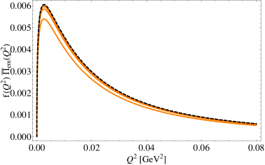
Figure 3: Comparison of the integral kernel $f(Q^{2})\bar{\Pi}_{\rm em}(Q^{2})$ which has a peak around $Q^{2}=m_{\mu}^{2}$: The dashed curve corresponds to the result including full contributions from the infinite tower of vector mesons, while four bold curves are obtained by integrating out the infinite tower at the levels of $n=1,2,3,4$. The dashed curve is almost (within about 1% deviation) reproduced when $n=4$. In the plot the number of flavors $N_{f}$ is taken to be 2.

In order to utilize the formula Eq. (3), we subtract $\Pi_{V}^{\rm ren}(0)$ to obtain

$$\bar{\Pi}_{V}(Q^{2}) \equiv \Pi_{V}^{\rm ren}(Q^{2})-\Pi_{V}^{\rm ren}(0)\,,$$ (25)

$$= \sum_{n=1}^{4}\frac{Q^{2}F_{V_{n}}^{2}}{(Q^{2}+M_{V_{n}}^{2})M_{V_{n}}^{4}}+{\cal O}(Q^{2}/(M_{V_{5}}^{2}))\,,$$

where $Q^{2}=-q^{2}$ is Euclidean momentum-squared. Note that the dependence of the renormalization scale $\mu$ has been removed.

Let us now evaluate $\bar{\Pi}_{V}$ of Eq. (25) numerically. Looking at Eq. (25), to this aim, we see that all we need to do is calculate the values of the vector meson poles $M_{V_{n}}$ and their pole residues $(F_{V_{n}}/M_{V_{n}}^{2})$ for each $n=1,2,3,4$. We first notice that the mass hierarchy of vector mesons are completely determined by locations of zeros given as $J_{0}(z_{m}M_{V_{n}})=0$ as seen from Eq. (13). Especially, for $n=1,2,3,4$, we have

$$z_{m}M_{V_{1}}=2.405\,,\qquad z_{m}M_{V_{2}}=5.520\,,$$

$$z_{m}M_{V_{3}}=8.654\,,\qquad z_{m}M_{V_{4}}=11.792\,.$$ (26)

Therefore, once the lowest pole is identified with the $\rho$ meson pole, i.e., $M_{V_{1}}=M_{\rho}=0.775\,[{\rm GeV}]$ Amsler:2008zz which fixes $z_{m}=3.101\,[{\rm GeV}]^{-1}$, we can obtain a set of the vector meson masses (in unit of GeV);

$$M_{V_{1}}=0.775\quad({\rm fit})\,,\qquad M_{V_{2}}=1.779\,,$$

$$M_{V_{3}}=2.788\,,\hskip 55.0ptM_{V_{4}}=3.802\,,$$ (27)

in which the values of $M_{V_{2}},M_{V_{3}}$ are compared to the empirical ones Amsler:2008zz , $M_{\rho_{2}}|_{\rm exp}=1.45$ and $M_{\rho_{3}}|_{\rm exp}=1.70$ in unit of GeV. We next turn to calculating the pole residues $F_{V_{n}}/M_{V_{n}}^{2}$ expressed as in Eq. (22). Note that the overall factor $(1/g_{5}^{2})$ of Eq. (22) is determined by considering a fit with the expression derived from the operator product expansion of $\Pi_{V}(Q^{2})$, and it is fixed as

$$\frac{1}{g_{5}^{2}}=\frac{N_{c}}{12\pi^{2}}\,.$$ (28)

For $n=1,2,3,4$, the values of $F_{V_{n}}/M_{V_{n}}^{2}$ of Eq. (22) are then calculated up to the overall factor as

$$\frac{F_{V_{1}}}{M_{V_{1}}^{2}}\cdot(\sqrt{N_{c}/12\pi^{2}})^{-1}=1.133\,,\qquad\frac{F_{V_{2}}}{M_{V_{2}}^{2}}\cdot(\sqrt{N_{c}/12\pi^{2}})^{-1}=-0.753\,,$$

$$\frac{F_{V_{3}}}{M_{V_{3}}^{2}}\cdot(\sqrt{N_{c}/12\pi^{2}})^{-1}=0.602\,,\qquad\frac{F_{V_{4}}}{M_{V_{4}}^{2}}\cdot(\sqrt{N_{c}/12\pi^{2}})^{-1}=-0.516\,.$$ (29)

Now we are ready to evaluate the HLO contribution to the muon anomalous magnetic moment $a_{\mu}^{\rm HLO}$. We shall focus on a two-flavor ($N_{f}=2$) HLO contribution, coming from the lightest two flavors $(u,d)$, and then compare the predicted value of $\alpha_{\mu}^{\rm HLO}$ with that estimated from the new BABAR data on the $e^{+}e^{-}\to\pi^{+}\pi^{-}$ events detected in a range of center of mass energies $2m_{\pi}\leq\sqrt{s}\leq 1.8$ GeV Aubert:2009fg . Taking into account Eq. (9) and substituting $\bar{\Pi}_{V}$ of Eq. (25) into the formula Eq. (3), using the theoretical values for the vector meson poles and their pole residues listed in Eqs.(27) and (29), we obtain

$$a_{\mu}^{\rm HLO}|^{N_{f}=2}_{\rm AdS/QCD}=470.5\times 10^{-10},$$ (30)

which agrees, within 30% errors, with the currently updated value Aubert:2009fg

$$a_{\mu}^{\rm HLO}[\pi\pi]|_{\rm BABAR}=(514.1\pm 3.8)\times 10^{-10}\,.$$ (31)

We expect that the $1/N_{c}$ corrections together with the isospin-breaking corrections could make up for the discrepancy between the values of Eq. (30) and Eq. (31).

V Discussion

We have calculated the hadronic leading correction (HLO) to the muon magnetic anomaly with two light flavors. The result is compared with a recently updated HLO value Davier:2009zi , estimated by including not only the BABAR new $e^{+}e^{-}\to\pi^{+}\pi^{-}$ data Aubert:2009fg but also the other experimental data involving other inclusive decay processes in which multi-hadrons more than two $\pi$s, such as $2\pi^{0}\pi^{+}\pi^{-}$, $2\pi^{+}2\pi^{-}$, are included in the final states, as well as some exclusive decay processes. From a theoretical point of view, those multi-hadronic decaying processes are thought to be dominated by higher order contributions of meson-loops in the large $N_{c}$ expansion. However, those higher order corrections have not been achieved in the present holographic framework which is based on the holographic correspondence, established only at the large $N_{c}$ limit. It is not adequate, therefore, to compare the result obtained from our present holographic calculation with that deduced from data involving such those decaying processes.

Similarly, we have not compared with the value estimated based on lattice calculation Blum:2002ii with the staggered fermions of $N_{f}=3$, because the value of Ref. Blum:2002ii includes a part of the meson-loop contributions.

We suspect that incorporation of $1/N_{c}$ corrections as done in Ref. Harada:2006di might make it possible to compare with these references.

V.1 Acknowledgements

We thank M. Drees and M. Hayakawa for useful comments and informing us of the references Aubert:2009fg ; Davier:2009zi and Aoyama:2008gy , respectively. The work of D. K. H. and S. M. was supported by the Korea Research Foundation Grant funded by the Korean Government (KRF-2008-341-C00008) and D. Kim was supported by the KRF grant (KRF-2008-313-C00162).

References

• (1) :. B. Aubert [The BABAR Collaboration], arXiv:0908.3589 [hep-ex].
• (2) M. Davier, A. Hoecker, B. Malaescu, C. Z. Yuan and Z. Zhang, arXiv:0908.4300 [hep-ph].
• (3) T. Blum and S. Chowdhury, Nucl. Phys. Proc. Suppl.  189, 251 (2009).
• (4) E. de Rafael, Phys. Lett.  B 322, 239 (1994) [arXiv:hep-ph/9311316].
• (5) E. Pallante, Phys. Lett.  B 341, 221 (1994) [arXiv:hep-ph/9408231].
• (6) J. Erlich, E. Katz, D. T. Son and M. A. Stephanov, Phys. Rev. Lett.  95, 261602 (2005) [arXiv:hep-ph/0501128]:
• (7) L. Da Rold and A. Pomarol, Nucl. Phys.  B 721, 79 (2005) [arXiv:hep-ph/0501218];
• (8) D. K. Hong, T. Inami and H. U. Yee, Phys. Lett.  B 646, 165 (2007) [arXiv:hep-ph/0609270].
• (9) T. Sakai and S. Sugimoto, Prog. Theor. Phys.  113, 843 (2005) [arXiv:hep-th/0412141].
• (10) D. K. Hong, M. Rho, H. U. Yee and P. Yi, Phys. Rev.  D 76, 061901 (2007) [arXiv:hep-th/0701276]; D. K. Hong, H. C. Kim, S. Siwach and H. U. Yee, JHEP 0711, 036 (2007) [arXiv:0709.0314 [hep-ph]]; K. Ghoroku, N. Maru, M. Tachibana and M. Yahiro, Phys. Lett.  B 633, 602 (2006) [arXiv:hep-ph/0510334].
• (11) D. K. Hong and D. Kim, Phys. Lett.  B 680, 480 (2009) [arXiv:0904.4042 [hep-ph]].
• (12) C. Aubin and T. Blum, Phys. Rev.  D 75, 114502 (2007) [arXiv:hep-lat/0608011].
• (13) T. Blum, Phys. Rev. Lett.  91, 052001 (2003) [arXiv:hep-lat/0212018].
• (14) T. Aoyama, M. Hayakawa, T. Kinoshita, M. Nio and N. Watanabe, Phys. Rev.  D 78, 053005 (2008) [arXiv:0806.3390 [hep-ph]].
• (15) L. Patino and G. Toledo, arXiv:0901.4773 [hep-th].
• (16) M. Bianchi, D. Z. Freedman and K. Skenderis, Nucl. Phys.  B 631, 159 (2002) [arXiv:hep-th/0112119].
• (17) K. Skenderis, Class. Quant. Grav.  19, 5849 (2002) [arXiv:hep-th/0209067].
• (18) C. Amsler et al. [Particle Data Group], Phys. Lett.  B 667, 1 (2008).
• (19) M. Harada, S. Matsuzaki and K. Yamawaki, Phys. Rev.  D 74, 076004 (2006) [arXiv:hep-ph/0603248].